
Optimizing the best play in basketball using deep learning
Abstract
In a close game of basketball, victory or defeat can depend on a single shot. Being able to identify the best player and play scenario for a given opponent’s defense can increase the likelihood of victory. Progress in technology has resulted in an increase in the popularity of sports analytics over the last two decades, where data can be used by teams and individuals to their advantage. A popular data analytic technique in sports is deep learning. Deep learning is a branch of machine learning that finds patterns within big data and can predict future decisions. The process relies on a raw dataset for training purposes. It can be utilized in sports by using deep learning to read the data and provide a better understanding of where players can be the most successful.
In this study the data used were on division I women’s basketball games of a private university in a conference featuring top 25 teams. Deep learning was applied to optimize the best offensive play in a game scenario for a given set of features. The system is used to predict the play that would lead to the highest probability of a made shot.
1Introduction
The increasing interest in sports analytics over the last two decades can be attributed to advances in technology where data has been used by teams and individuals to gain a competitive advantage (Goldsberry, 2012). Statistics have always played a role in sport, but the use of predictive analysis has increased in recent years. The volume of data collected for each game makes a big data problem since it is not readily feasible to gain meaningful insights from raw data. Data driven decision-making is being incorporated in different aspects of sports from gambling, fantasy leagues, to improving team dynamics and performance, decision making, preventing injuries, etc. Deep learning and machine learning techniques are critical techniques since data is unstructured and lacks context.
Deep learning is a branch of machine learning that identifies patterns within big data and can be used to predict future decisions. The process relies on a raw data for training purposes (Rangel et al., 2019). Deep learning can be used to give teams better insights on which players to select, predict an opponent’s actions, determine how to train players, and prevent injuries, and provide management a better understanding on ways to enhance revenue and fan engagement.
As a global sport, research on aspects of the game of basketball are valuable in its improvement. Traditional measurement of game performance has been based on statistics that are collected and displayed in a box score (Skinner and Guy, 2015). More recently, data analytics in basketball have used machine learning to predict the outcome of an NBA game using Naive Bayes and Artificial Neural Networks (Cao, 2014), or visualization of made and missed shots via shot charts within a game (Reich et al., 2006). There has been research on using deep learning to predict the defensive play of the opponent given the ball and offensive players movement (Zuccolotto and Manisera, 2020; Chen et al., 2018; Hsieh et al., 2019). However, these models don’t generate the offensive strategy and the input of player movement is simplified that doesn’t necessary capture the realistic output (Mgaya et al., 2020). In another research Recurrent Neural Networks were used to predict whether a three-point shot’s success given the position data and game clock (Shah and Romijnders, 2016). Shot charts demonstrate where a team has made a shot with a circle and missed a shot with an X with respect to the location of a shot. These charts can be useful in determining where most of the shots have been made for each team, however they do not provide additional insights beyond a location within the court. To extend deeper using data analytics, more information about the shot needs to be integrated, rather than location alone. In another study to help evaluate shooting within the NBA, Effective Shot Quality (ESQ) was created to help improve Effective Field Goal percentage (EGF) (Chang et al., 2014). ESQ considers factors such as the angle of the defender to the shooter, defender distance, shot angle etc.
Player performance analysis is a hot topic and has been the focus of researchers in recent years (Zuccolotto and Manisera, 2020; Terner and Franks, 2021; Zuccolotto et al., 2021; Sandri et al., 2020; Ntasis, 2019). Sandri et al work addresses shooting performance, with a special focus on performance variability using Markov switching models. They analyzed shooting performance and investigated its relationship to team line-up and team performance (Sandri et al., 2020). Migliorati (2020) presented a model to identify the success of a game. They used box office analytics and four factor model and performed machine learning using CART and Random forests. They identified the most important factors in predicting the outcome of a game. Zuccolotto et al. (2018) studied the outcome a shot under high pressure conditions. Their work shows that the situation most impacting the scoring probability is when the shot clock is about to expire and, when the player has missed the previous shot. Ntasis (2019) analyzed the NBA 2019 champion matches to identify the optimal strategy based on each player’s return during the game. The findings show that under convex risk measures, coaches can optimize players returns. Their system can be used to identify the best player selection in different circumstances. Metulini et al. (2017) used Cluster Analysis and split the course into several separate time-periods to identify the player positions and spacing in defensive and offensive plays to analyze the transition probability between different groups of players.
In basketball, offensive possessions are arguably one of the most valued components of the game. In a close game, the last few possessions often determine if a team wins or loses (Christmann et al., 2018). The last play of a game can completely alters the outlook of how a team played and/or impact a fan’s perceptions about a game (Bashuk, 2012). Turnovers often limit a team’s chance to score and gives the opposing team extra opportunities. Missed shots in a close game can be just as costly as turnovers. A successful possession results in a player taking a reasonably high percentage shot (Skinner, 2012).
Expected Possession Value (EPV) of players is another measure that has been used. Cervone et al. proposed a framework to estimate the EPV which reacts to every on-court movement and action and is the expected number of points the offense will score, given the spatial configuration of the players and ball at time during the possession (Cervone et al., 2014). The EPV assigns a point to every option available and allows evaluating the decisions that players made on court. EPV allows data analysis to focus on decision making and opportunity creation that were not possible before. EPV is not only used in basketball but in other sports such as soccer and rugby (Fernandez et al., 2021; Sawczuk et al., 2021).
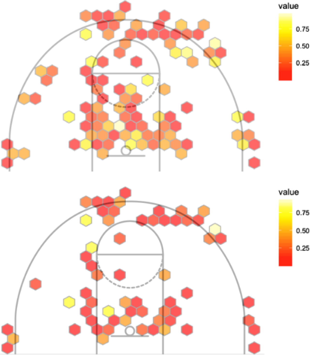
There are numerous statistics tracked in a basketball game. One of the most significant is Field Goal Percentage. In many instances, someone with the highest Field Goal Percentage or the most Field Goals Made on the team is the person most likely to take a game winning shot in a close game. In the NBA, the average 3 points Field Goal Percentage has been approximately 35% for the past 20 years (Marty and Lucey, 2017). NCAA Division 1 women’s basketball had an average 3 points percentage around 31% and an average 2 points percentage of 40%. Previous research found that a player who made a shot the possession before is more likely to take the next shot (Attali. 2013). In Fig. 1, the shot chart on the left shows the traditional probability distribution density that describes the likelihood of players making their shots for a given location on the court. The shot chart on the right (Fig. 1) shows the optimized model which considers the correlation among the dataset and is calculated based on constant defensive attribute values.
Fig. 1
Graphical depiction of an offensive likelihood of making shot; Likelihood of making a shot based on the constraints on the model’s defensive.
In this paper we perform data mining in basketball to identify the best offensive play based on a set of features. Our deep learning model predicts the offensive features along with the best player to take the shot. The Expected Possession Value (EPV) of each player is used to identify the players to perform a selected play that will result in the greatest probability of a made basket. The type of questions that our framework can answer are:
• During an offensive possession, given an opponent’s defensive scheme, what is the play scenario that has the highest probability of success?
• Who is the best player to take a shot?
• At each point in the game what is the EPV of each player?
In other words, assume 5 seconds remains on the shot clock. Timeout is requested. The developed system can predict: what is the best play? Who should take the shot? Who are the other players that should be in the game based on the opponent’s defensive scheme?
2Data
The data used is on division I 2018–2021 season of one college women’s basketball team. The feature vector consists of a set of 21 attributes each of which is listed on Table 1. The attributes can be broken down into 3 parts. One group of attributes deal with the characteristics of the play, a second set of features focus on the game and score status and the last group of features consider the play and the performance outcome by using the shots taken and the shots made during the game. For the last group of features we used box score features to summarize the status of a player’s outcome.
Table 1
Feature description
| Attributes | Description |
| Player | Player who takes the shot |
| Play | The play that was run to get a player a shot |
| Defense Type | Whether the opponent’s defense is in a zone or man-to-man |
| Defender Position | The location of defender |
| Screen | If a screen was used to get the player an open shot |
| Quarter | The quarter the shot was taken in |
| Seconds on Shot Clock | Number of seconds left on the shot clock |
| Number of Defenders | The number of defenders in the half court at the time of the shot |
| Location | The location shot was taken (out of 11 sports) |
| Hand | right or left |
| Shot type | Labeled as lay-up, dribble jumper, spot up, turn-around jumper (TAJ), floater, step back, or spin shot |
| Passes in half court | Number of passes prior to the shot |
| Minutes left in quarter | Minutes remaining in the quarter |
| 2PA | 2 points filed goals attempted |
| 2PM | 2 points filed goals made |
| 3PA | 3 points filed goals attempted |
| 3PM | 3 points filed goals made |
| FTA | free throws attempted |
| FTM | free throws made |
| Point difference | The point different of the game |
| Result | Make or miss |
Based on these attributes, the model is trained to predict the ‘Make’ or ‘Miss’ of a shot in a given game situation. Data preprocessing consists of cleaning and reduction. In the data cleaning step, we deal with inconsistent, noisy, and missing data.
3Methodology
This paper introduces a new method for the field of basketball analytics by identifying the best game plan at time t given a specific game scenario. Our model is used to predict the best shooter, offensive play, and the top 4 players to support the play. The top 4 players are selected based on the maximum expected number of points given the location of the players.
3.1Deep learning –Who is the shooter and what is the play?
Previously, the best shooters were predicted by data scientists using a factorization machine model (Wright et al., 2016) and Adversarial Multiagent Trajectories (Harmon et al., 2016). Deep learning can be applied to shots in basketball to predict the best shooter and the optimal play to run in specific game situations. With the use of these predictions, coaches can learn how to optimize each possession within a game, by choosing the best approach to taking a shot.
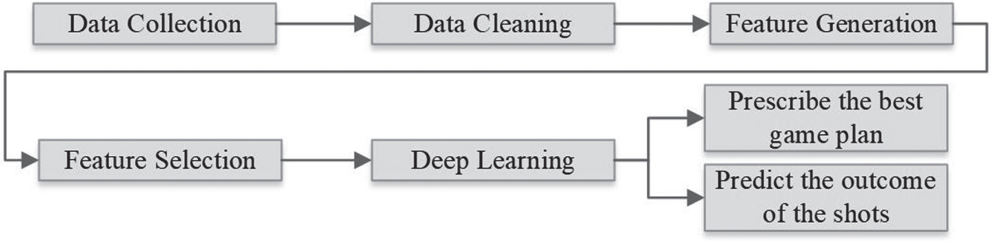
After generating the feature vector for each shot, Python and RapidMiner were used for data mining. The deep learning model was used to predict the best play based on our defined feature vector. An overview of the methodology is presented in Fig. 2.
Fig. 2
Proposed framework for predicting the best play using deep learning.
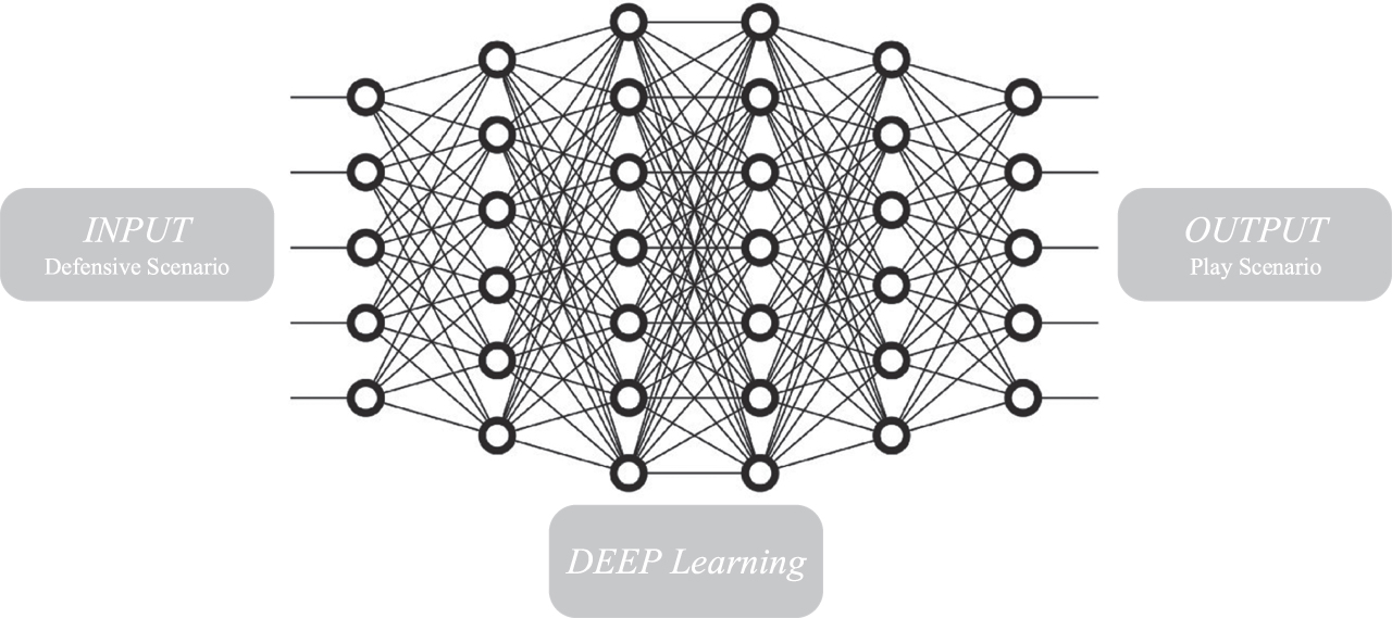
Deep learning uses the imported data as a training tool to predict future outcomes of shots (Fig. 3). The process of deep learning is as follows: first, the data is retrieved, then the data is processed where the target column is identified. After this, if the data has any missing values, those will be replaced with the average of the column. However, in our current model all data was cleaned prior to modelling, so no missing values were included in the input. The data is then filtered and sent to deep learning to train the model. Finally, the data is sent to the model simulator, where it can be applied, and the result can be predicted.
Fig. 3
Deep learning framework.
After collecting data and an explanatory data analysis, feature selection and extraction is performed. Using a prediction model, we built a machine learning model to predict the make/miss values based on the other features. We then utilized supervised learning to train the model. We evaluated the accuracy for each pattern recognition model described in Table 2 and we chose a multi-level neural network for learning non-linear relationships. As the deep learning algorithm is computationally expensive, we opted for a 80:20 split between training and test data. The multi-layer feed-forward artificial neural network model was built using H2O deep learning algorithm and was set up with a rectifier activation function and ten epochs.
Table 2
Different model methods with accuracy and total time
| Model | Accuracy | Standard Deviation | Total Time | Training Time | Scoring Time |
| Naive Bayes | 56.7% | ±6.1% | 165 ms | 5 ms | ∼0 ms |
| Generalized Linear Model | 59.4% | ±5.5% | 198 ms | 147 ms | 8 ms |
| Logistic Regression | 57.8% | ±8.4% | 211 ms | 147 ms | 8 ms |
| Fast Large Margin | 58.3% | ±6.8% | 368 ms | 5 ms | ∼0 ms |
| Deep Learning | 64.4% | ±8.4% | 826 ms | 1 s | 31 ms |
| Decision Tree | 61.9% | ±9.1% | 183 ms | ∼0 ms | ∼0 ms |
| Random Tree | 66.3% | ±7.3% | 4 s | 131 ms | 78 ms |
The model predicts the actual result of the shot with an accuracy of 75.6%. The f-measure of the model is 84.62%. In other words, using the attributes listed on Table 1, the model predicts the chosen play (player, shot type, location, and play) will be successful with 75.6% certainty.
As shown in Table 2, the training time for the Deep Learning model is 826 milliseconds. Deep learning is the second most accurate model, behind Random Tree. However, Random Tree requires 4 seconds to create the model. 4 seconds is typically too long to create a model in a time sensitive game situation. A team has a limited amount of time during stoppage of play during a timeout and selecting attributes also requires time as well. That is why Deep Learning is likely the best model methods based on accuracy and total time.
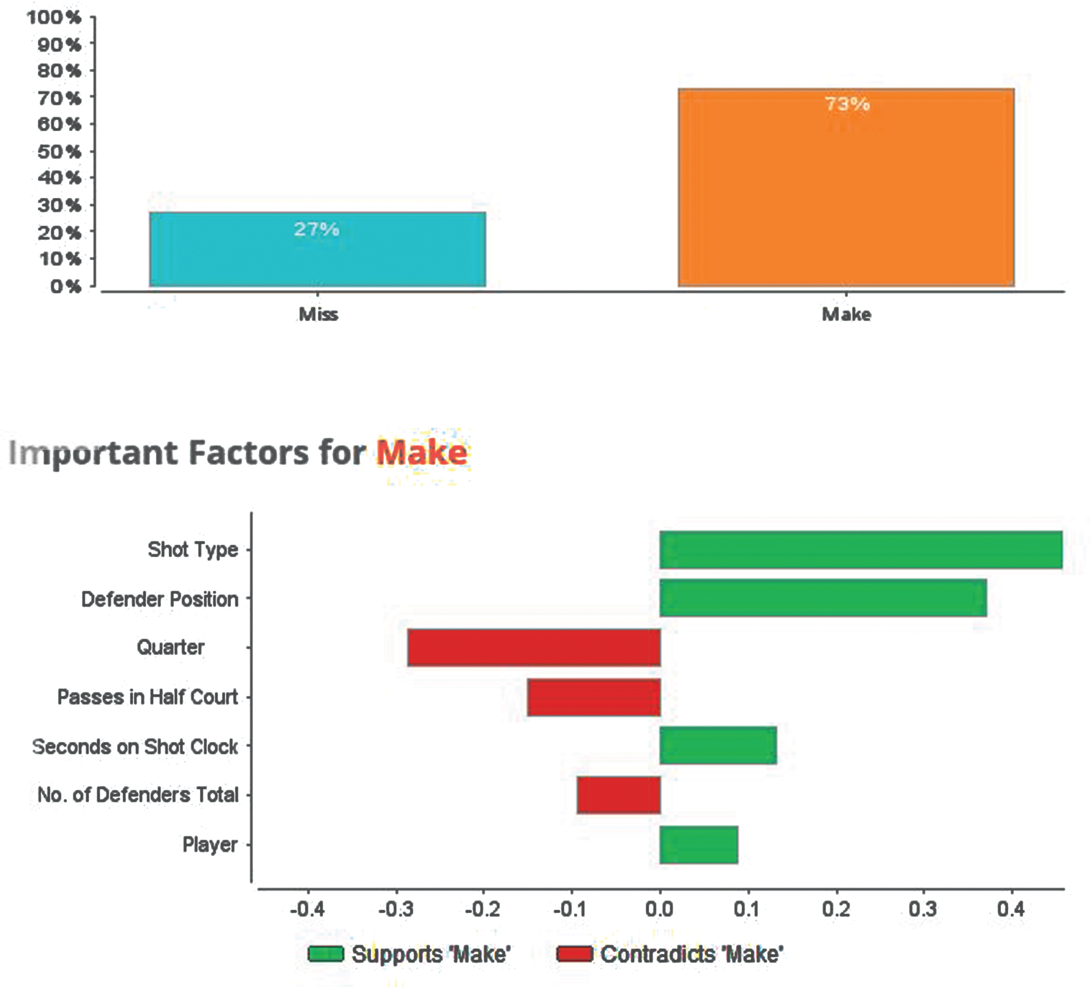
Once our model was created, we used the RapidMiner’s recommender system to specify the best play based on defensive characteristics and the statistics and status of the game. Table 3 and Fig. 4 show a sample feature vector as well as the result of deep learning model. Given the attributes presented in Table 2, the play scenario is predicted with a likelihood of 73% chance of success.
Table 3
Overview of the system
| Attributes | Results |
| Defense Type: Man | Player: 51 |
| Defender Position: Contested | Shot type: Spot up |
| Passes in Half Court: 2 | Location: 8 |
| Screen: No | Play: Picket fence |
| Quarter: 4 | |
| Seconds on Shot Clock: 20 | |
| Time left in quarter: 5 minutes | |
| Location: 5 | |
| Number of Defenders | |
| in half court: 5 | |
| 2PA: 10 | |
| 2PM: 8 | |
| 3PA: 5 | |
| 3PM:1 | |
| FTA:4 | |
| FTM:4 | |
| Point difference: –2 |
Fig. 4
System result.
3.2Expected possession value –Who should play to support the shooter?
In the second phase of the model, the goal is to select the other 4 players to accompany the shooter for a successful play. For this purpose, the EPV of players is calculated and updated throughout the game. EPV is a measure for opportunity creation and decision making of players throughout the game. If the ball does not get to the selected player in 4.1 then we want to make sure that the other players will be able to assist for a successful shot. For this reason, we used EPV to identify the best players that could assist with the selected play in the previous stage to ensure the highest probability of success. To calculate the EPV, tracking game data is used. Each data point represents a time point and consists of values such as: time, quarter, shot clock, game clock, play, player number and player possession location (x, y). EPV is calculated using Monte Carlo simulation (Equation 1).
(1)
Table 4
EPV of players
| Player | EPV |
| 1 | 1.65 |
| 2 | 1.45 |
| 3 | 1.38 |
| 4 | 1.21 |
| 5 | 1.05 |
| 6 | 1.03 |
| 7 | 1.00 |
| 8 | 0.90 |
| 9 | 0.70 |
Table 5 shows EPV of players for the scenario presented in Table 3. EPV results are used to select the other 4 players to accompany the chosen shooter.
4Discussion
The model is designed to predict the best play in a game situation. Besides defender position and number of defenders position, location, passes in the half court, history of shorts, and time remaining on the shot clock have a significant impact on the chances of a made shot. In general, the further the shot is away from the basket, the lower the chances of a made shot. Passes in the half court have an important impact on the likelihood of success since most basketball plays involve movement of the ball to get the defense to move. Getting the defense to move and shift can help change the spacing between players and create better opportunities for shots.
Time remaining on the shot clock has the largest correlation to a Make or Miss. Time remaining is significant in basketball since it adds pressure to the shooter, causing players to rush and potentially leads to poor shot selection. When time remaining on the shot clock is relatively high, the likelihood of a made shot tends to increase. Whereas, when time remaining on the shot clock is low, the likelihood of a made shot tends to decrease. In the model, when the shot clock is at 20 seconds for the scenario described in Table 2, the chances of a made shot are 73%. When the shot clock is at 6 seconds the chances of a made shot are 13%. This also demonstrates that the model understands the importance of the shot clock in basketball.
Although the model can be used to show the probability of a made shot in terms of percentage, the primary goal of the model is to use it in a game situation where a team needs a last second shot. For instance, if a team is behind by three points and have one more possession to take a shot, a coach can turn to this model to identify a play and the shooter with the best chances of making the last shot. The coach is also able to identify the 4 other players to perform the play by selecting the players with the highest real-time EPV based on in-game information as well as a player’s past performance in prior games.
5Future work
We made a few assumptions to simplify the model. Further refinement of the model could define a more precise outcome for the coach’s playbook. For instance, we didn’t consider transitional movement in calculating the EPV of players, we also didn’t consider defensive attributes of players on the opposing team. In addition, for future research, it seems desirable to model the conditional probability based on the selected shooter and choose the other players not only based on individual EPVs but also consider the chemistry of the shooter and other players. Also, for future work we will consider the options of winning vs tie shot in cases where the team in only 2 points behind.
References
1 | Attali, Y. , (2013) , Perceived hotness affects behavior of basketball players and coaches, Psychological Science, 24: (7), 1151–1156. |
2 | Bashuk, M. , 2012, March. Using cumulative win probabilities to predict NCAA basketball performance, In Proceedings of the MIT Sloan Sports Analytics Conference, 1–10. |
3 | Cao, C. , (2012) , Sports data mining technology used in basketball outcome prediction. Master dissertation, Dublin Institute of technology, Ireland, (2012) . |
4 | Cervone, D. , D’Amour, A. , Bornn, L. and Goldsberry, K. , (2014) , February. Pointwise: Predicting points and valuing decisions in real time with NBA optical tracking data, In Proceedings of the 8th MIT Sloan Sports Analytics Conference, Boston, MA, USA, 28, 3. |
5 | Chang, Y.H. , Maheswaran, R. , Su, J. , Kwok, S. , Levy, T. , Wexler, A. and Squire, K. , (2014) , February. Quantifying shot quality in the NBA, In Proceedings of the 8th Annual MIT Sloan Sports Analytics Conference. MIT, Boston, MA. |
6 | Chen, C.Y. , Lai, W. , Hsieh, H.Y. , Zheng, W.H. , Wang, Y.S. and Chuang, J.H. , 2018, October. Generating defensive plays in basketball games, In Proceedings of the 26th ACM international conference on Multimedia, 1580–1588. |
7 | Christmann, J. , Akamphuber, M. , Müllenbach, A.L. and Güllich, A. , (2018) , Crunch time in the NBA–The effectiveness of different play types in the endgame of close matches in professional basketball, International Journal of Sports Science & Coaching, 13: (6), 1090–1099. |
8 | Fernández, J. , Bornn, L. and Cervone, D. , 2021, A framework for the fine-grained evaluation of the instantaneous expected value of soccer possessions, Machine Learning, pp. 1–39. |
9 | Goldsberry, K. , (2012) , Courtvision: New visual and spatial analytics for the NBA, MIT Sloan Sports Analytics Conference, 9: , 12–15. |
10 | Harmon, M. , Ebrahimi, A. , Lucey, P. and Klabjan, D. , 2016, Predicting shot making in basketball learnt from adversarial multiagent trajectories, arXiv preprint arXiv:1609.04849. |
11 | Hsieh, H.Y. , Chen, C.Y. , Wang, Y.S. and Chuang, J.H. , 2019, October. Basketballgan: Generating basketball play simulation through sketching, In Proceedings of the 27th ACM International Conference on Multimedia, 720–728. |
12 | Marty, R. and Lucey, S. , 2017, A data-driven method for understanding and increasing 3-point shooting percentage, In Proceedings of the 2017 MIT Sloan Sports Analytics Conference. |
13 | Metulini, R. , Manisera, M. and Zuccolotto, P. , 2017, Space-time analysis of movements in basketball using sensor data, In Statistics and Data Science Proceedings: new challenges, new generations, Firenze University Press, arXiv preprint arXiv:1707.00883 |
14 | Mgaya, G.B. , Liu, H. and Zhang, B. , 2020, A Survey on Applications of Modern Deep Learning Techniques in Team Sports Analytics. In Proceedings of the 12th International Conference of Soft Computing and Pattern Recognition, 434–443. |
15 | Migliorati, M. , (2020) , Detecting drivers of basketball successful games: an exploratory study with machine learning algorithms, Electronic Journal of Applied Statistical Analysis, 13: (2), 454–473. |
16 | Ntasis, L. , (2019) , Optimization techniques for basketball players under the convex risk measures. Journal of Human Sport and Exercise, Journal of Human Sport and Exercise, 14: (5proc), S2435–S2440. |
17 | Rangel, W. , Ugrinowitsch, C. and Lamas, L. , (2019) , Basketball players’ versatility: Assessing the diversity of tactical roles, International Journal of Sports Science & Coaching, 14: (4), 552–561. |
18 | Reich, B.J. , Hodges, J.S. , Carlin, B.P. and Reich, A.M. , (2006) , A spatial analysis of basketball shot chart data, The American Statistician, 60: (1), pp. 3–12. |
19 | Sandri, M. , Zuccolotto, P. and Manisera, M. , (2020) , Markov switching modelling of shooting performance variability and teammate interactions in basketball, Journal of the Royal Statistical Society: Series C (Applied Statistics), 69: (5), 1337–1356. |
20 | Sawczuk, T. , Palczewska, A. and Jones, B. , 2021. Development of an expected possession value model to analyse team attacking performances in rugby league, arXiv preprint arXiv:2105.05303. |
21 | Shah, R. and Romijnders, R. , 2016, Applying deep learning to basketball trajectories. arXiv preprint arXiv:1608.03793, 1–4. |
22 | Skinner, B. , (2012) , The problem of shot selection in basketball, PloS one, 7: (1), e30776. |
23 | Skinner, B. and Guy, S.J. , (2015) , A method for using player tracking data in basketball to learn player skills and predict team performance, PloS one, 10: (9), pp. e0136393. |
24 | Terner, Z. and Franks, A. , (2021) , Modeling player and team performance in basketball, Annual Review of Statistics and Its Application, 8: , 1–23. |
25 | Wright, R.E. , Silva, J and Kaynar-Kabul, I. , 2016, Shot recommender system for NBA coaches. In KDD Workshop on Large-Scale Sports Analytics. |
26 | Zuccolotto, P. , Sandri, M. and Manisera, M. , (2021) , Spatial Performance Indicators and Graphs in Basketball, Social Indicators Research, 156: (2), 725–738. |
27 | Zuccolotto, P. and Manisera, M. , (2020) , Basketball data science: with applications in R. CRC Press. |
28 | Zuccolotto, P. , Manisera, M. and Sandri, M. , (2018) , Big data analytics for modeling scoring probability in basketball: The effect of shooting under high-pressure conditions, International Journal of Sports Science & Coaching, 13: (4), 569–589. |


