Predicting the winning percentage of limited-overs cricket using the Pythagorean formula
Abstract
The Pythagorean Win-Loss formula can be effectively used to estimate winning percentages for sporting events. This formula was initially developed by baseball statistician Bill James and later was extended by other researchers to sports such as football, basketball, and ice hockey. Although one can calculate actual winning percentages based on the outcomes of played games, that approach does not take into account the margin of victory. The key benefit of the Pythagorean formula is its utilization of actual average runs scored and actual average runs allowed. This article presents the application of the Pythagorean Win-Loss formula to two different types of limited-overs cricket formats, namely One Day International cricket (ODI) and Twenty20 cricket. The data for the application was used from the matches played by the top 10 International Cricket Council (ICC) members who participated in the 2019 ICC Cricket World Cup. For matches for which the second batting team won, runs scored were estimated by considering the remaining amount of resources, based on the Duckworth–Lewis method.
1Introduction
The Pythagorean Win-Loss formula, which was developed by Bill James in the early 1980s, is a sports analytics formula that can be effectively used to calculate winning percentages for sporting events. This calculation is based on the average number of runs scored (RS) and the average number of runs allowed (RA) by a team. In particular, the Pythagorean Win-Loss formula with Pythagorean exponent γ is given as follows.
(1)
One can directly predict the expected number of matches a team will win in a future series based on the observed winning percentage for the period so far. For example, the observed winning percentage of the matches played from the end of the last ODI cricket world cup to the beginning of the next world cup can be used to predict the number of matches expected to be won by a team in the next world cup. One can do a better prediction using the Pythagorean winning percentage, which can be calculated using Equation (1). The added value of the Pythagorean winning percentage over the regular winning percentage is that it takes into account more accurate defensive and offensive strengths of the teams by using the actual runs scored and actual runs allowed. The regular winning percentage does not have a way to accommodate the actual scores and it uses the binary outcome of a game (win or lose). However, with the appropriate Pythagorean exponent (γ), the Pythagorean winning percentage utilizes additional information of the actual scores, which in return provides predictions that are more practical. Initially, this formula was used by baseball statisticians, and the Pythagorean exponent was assumed to be 2. However, a later empirical study by Miller (2006) has shown that a better agreement can be attained when the exponent was about 1.82. Miller (2006) was also the first to show the theoretical justification of the formula by assuming independent Weibull distributions for runs scored and runs allowed. Often this formula is used to predict the end of the season standing of a team, based on its performance halfway through the season (Miller, 2006). Several researchers have used this Pythagorean formula to determine the winning percentages of other sports as well by finding appropriate γ values for the specific sport. According to Schatz (2003), statistician Daryl Morey’s research has proven that the Pythagorean formula can be applied to all the major sports, with different exponents for each; in particular, he has shown that the γ value for National Football League (NFL) was about 2.37. Dayaratna and Miller (2012) have shown that the Pythagorean Win-Loss formula can be used as an evaluative tool in hockey. They have further shown that the maximum likelihood estimate of γ is almost always slightly above 2 for all three National Hockey League (NHL) seasons they considered. Oliver (2004) has shown that the appropriate value of γ for basketball is around 14. Rosenfeld et al. (2010) have used the formula to predict overtime outcomes in the National Football League (NFL), Major League Baseball (MLB), and National Basketball Association (NBA). Heumann (2016) described a new version of the Win-Loss formula, which was called pairwise Pythagorean win. Chen and Li (2018) have introduced a shrinkage factor to increase the accuracy of the Pythagorean Win-Loss formula.
Application of the Pythagorean formula to cricket has been more limited, as the authors are aware of only a single relevant study. In that study, Vine (2016) used the Pythagorean formula to estimate the winning percentage of the Twenty20 Cricket Big Bash League, an Australian domestic competition. Vine (2016) has further shown that the appropriate γ value for the Twenty20 Cricket Big Bash League was 7.41. Vine (2006) also suggested that for the cases where the second batting team wins the match without using all the allocated resources, the dependency issue between runs scored and runs allowed could be eliminated by extrapolating the second team’s run total, by using the Duckworth–Lewis resources table. It is obvious that, as in any other sport, there could be a significant difference in the performance parameters between international level games and regional level games such as Big Bash League. Our effort in this paper is therefore to extend Vine’s results to international limited over cricket. Specifically, the objective of this paper is to calculate the winning percentage of the top 10 teams of the International Cricket Council (ICC); in particular, the goal is to estimate the appropriate Pythagorean exponent for both of the limited-over cricket formats, Twenty20 and One Day International (ODI).
1.1Limited-overs cricket
Cricket is one of the most popular games in the world, especially among Commonwealth countries. The three main types of cricket matches are test cricket, One Day International (ODI), and Twenty20. The two formats, ODI and Twenty20 cricket matches, have a limited number of overs and are known as limited-overs cricket. An over consists of six deliveries from bowler to batsman. An innings in ODI and Twenty20 consists of 50 overs and 20 overs respectively. For all major cricket formats, a team consists of 11 players, and the match starts with a coin toss to determine the first batting team. That team’s goal is to score the maximum number of runs by using the available resources (number of overs and wickets). The second batting team then attempts to score at least one more run than the first team’s total. If they succeed, the second batting team wins the match, but if they fail, the first batting team wins.
Duckworth and Lewis (1998) introduced a way of revising targets for games that are shortened due to weather interruptions. This is the current method used by the ICC to revise the target for weather interrupted cricket matches. It is based on the idea that the batting team has two resources: (i) a certain number of overs to face and (ii) a limited number of wickets in hand. Based on a mathematical model, the Duckworth-Lewis method provides a table with the remaining percentage resources at any given stage of a game. For example, at the beginning, a team with all the wickets and all the overs remaining, has 100% of the resources. If it rains, and the game is delayed by several overs, then the team does not get the 100% resource available to that team. The Duckworth-Lewis method is used to calculate the revised target based on the remaining percentage of resources after the interruption is over. Complete details of the method can be found in Duckworth and Lewis (1998), which provides a two-way table for the available number of overs and the number of wickets lost, to ease calculations.
In particular, for our study, if the second batting team wins the match with wickets and overs are still remaining, their total will be extrapolated using the Duckworth-Lewis resources table, as suggested by Vine (2016). In cricket, when the second batting team surpasses the target score set by the first batting team, the game ends, and the second team is declared as the winner. However, had the second team been given the opportunity, it would have continued to score while using the remaining amount of resources allocated to it. When the game ends this way, using the second team’s actual scores as the runs scored distorts the true offensive strength of the second team. Therefore, it would be more appropriate to adjust the score incorporating the unused (remaining) amount of resources as well. This can be done using the Duckworth-Lewis method. In particular, the second team’s score can be extrapolated as if it was allowed to consume 100% of available resources. For details about the Duckworth-Lewis method, refer to Duckworth and Lewis (1998). Perera and Swartz (2013) also has an insightful discussion about using the Duckworth-Lewis method to analyze tactics in Twenty20 cricket.
The remainder of this paper is structured as follows. Section II describes the data used in this study. Section III describes the methodology used to determine the γ and the winning percentages. It also discusses the goodness of fit of the Weibull distribution and the validity of the assumption of independence between runs scored and runs allowed. Furthermore, it presents the data analysis and results. Section IV presents the conclusions. Throughout the paper, the terms runs scored and runs allowed are used in reference to the second batting team in order to facilitate the consistency of arguments.
2Description of data
In this study, we have used data from ODI matches played by the top 10 national teams of the International Cricket Council (ICC) during the time period between the 2015 and 2019 ICC World Cups. These teams are Afghanistan, Australia, Bangladesh, England, India, New Zealand, Pakistan, Sri Lanka, South Africa, and West Indies. For Twenty20 cricket, in order to have sufficient data, we used data for all matches played by the above 10 teams between 2012 and 2018. Matches with no results and matches shortened due to weather interruptions were removed from the analysis.
Descriptive statistics of total runs scored for ODI matches is shown in Table 1. It can be seen that the lowest total was 74 (Pakistan), and the highest was 512 (India). The lowest median score was 212 (West Indies), and the highest median score was 323 (England). Note that some of these scores were extrapolated scores by using the Duckworth-Lewis method for matches in which the second batting team won with overs and wickets are still remaining.
Table 1
Descriptive Statistics for Runs Scored in ODI Matches
| Team | Minimum | 1st quartile | Median | Mean | 3rd quartile | Maximum |
| AFG | 138 | 214 | 231 | 226 | 255 | 287 |
| AUS | 137 | 239 | 257 | 267 | 308 | 386 |
| BAN | 119 | 233 | 270 | 262 | 298 | 370 |
| ENG | 204 | 272 | 323 | 336 | 397 | 497 |
| IND | 158 | 249 | 304 | 306 | 340 | 512 |
| NZ | 79 | 227 | 284 | 272 | 323 | 484 |
| PAK | 74 | 219 | 271 | 265 | 307 | 366 |
| SA | 121 | 256 | 286 | 285 | 328 | 456 |
| SL | 124 | 187 | 249 | 240 | 296 | 338 |
| WI | 121 | 177 | 212 | 233 | 281 | 389 |
Descriptive statistics of total runs allowed in ODI matches is shown in Table 2. The highest total was 481 (Australia), and the lowest was 92 (New Zealand). The highest median was 316(Sri Lanka), and the lowest median was 229 (Afghanistan).
Table 2
Descriptive Statistics for Runs Allowed in ODI Matches
| Team | Minimum | 1st quartile | Median | Mean | 3rd quartile | Maximum |
| AFG | 197 | 205 | 229 | 234 | 261 | 279 |
| AUS | 116 | 246 | 281 | 274 | 307 | 481 |
| BAN | 162 | 245 | 263 | 269 | 311 | 369 |
| ENG | 150 | 228 | 274 | 274 | 305 | 381 |
| IND | 104 | 217 | 262 | 259 | 304 | 438 |
| NZ | 92 | 242 | 271 | 273 | 307 | 408 |
| PAK | 103 | 233 | 266 | 272 | 327 | 444 |
| SA | 149 | 192 | 246 | 247 | 296 | 371 |
| SL | 112 | 276 | 316 | 305 | 363 | 392 |
| WI | 113 | 260 | 301 | 287 | 329 | 418 |
Descriptive statistics of total runs scored in Twenty20 matches is shown in Table 3. These totals ranged from 60 (New Zealand and West Indies) to 333(New Zealand). Median scores ranged from 132 (Afghanistan) to 166(India). Again, some scores were extrapolated by using the Duckworth-Lewis method, for matches in which the second batting team won without using all the resources allocated to it.
Table 3
Descriptive Statistics for Runs Scored in Twenty20 Matches
| Team | Minimum | 1st quartile | Median | Mean | 3rd quartile | Maximum |
| AFG | 80 | 92 | 132 | 124 | 144 | 172 |
| AUS | 86 | 146 | 164 | 165 | 181 | 266 |
| BAN | 70 | 134 | 144 | 144 | 164 | 220 |
| ENG | 80 | 143 | 164 | 165 | 181 | 251 |
| IND | 79 | 145 | 166 | 164 | 182 | 244 |
| NZ | 60 | 137 | 154 | 153 | 167 | 333 |
| PAK | 74 | 126 | 144 | 144 | 158 | 201 |
| SA | 90 | 136 | 155 | 154 | 170 | 230 |
| SL | 87 | 122 | 146 | 145 | 171 | 242 |
| WI | 60 | 124 | 143 | 152 | 175 | 264 |
Table 4 shows the descriptive statistics for runs allowed in Twenty20 matches. The number of runs allowed is ranged from 67 (New Zealand) to 263 (Sri Lanka). Median scores ranged from 148 (Pakistan) to 171 (Bangladesh).
Table 4
Descriptive Statistics for Runs Allowed in Twenty20 Matches
| Team | Minimum | 1st quartile | Median | Mean | 3rd quartile | Maximum |
| AFG | 134 | 140 | 151 | 163 | 187 | 209 |
| AUS | 80 | 137 | 153 | 156 | 184 | 243 |
| BAN | 72 | 146 | 171 | 171 | 195 | 224 |
| ENG | 89 | 144 | 157 | 163 | 183 | 248 |
| IND | 82 | 129 | 159 | 154 | 172 | 245 |
| NZ | 67 | 143 | 169 | 162 | 183 | 214 |
| PAK | 89 | 133 | 148 | 149 | 168 | 211 |
| SA | 86 | 120 | 157 | 153 | 176 | 203 |
| SL | 81 | 130 | 155 | 156 | 175 | 263 |
| WI | 110 | 137 | 165 | 168 | 194 | 243 |
3Methodology
We applied the Pythagorean Win-Loss formula to cricket, following Miller (2006) assumption that runs scored and runs allowed follow independently distributed Weibull distributions with a common shape parameter. The probability density function of the Weibull distribution is given as follows.
(2)
where γ is the shape parameter, α is the scale parameter, and β is the location parameter.
As explained by Miller (2006), number of runs scored and the number of runs allowed in a given match follow independent Weibull distributions with parameters (αRS,β, γ) and (αRA, β, γ) respectively. By denoting the mean of runs scored as RS and mean of runs allowed as RA for a given team, we can show that
(3)
where RS = αRSΓ (1 + γ-1) + β and RA = αRAΓ (1 + γ-1) + β.
Therefore, the winning percentage of the team is given by,
(4)
We used both the maximum likelihood method and the least squares method for parameter estimation. The next subsection describes the parameter estimation and the other results using the Weibull models for runs scored and runs allowed.
3.1Parameter estimation and results
Similar to Vine (2016), runs of Twenty20 matches were split into bins to estimate the parameters of the Weibull distribution as follows.
Analogous split was used to create the following binning for ODI matches.
The same binning structures were used for each team, with both the least squares method and the maximum likelihood method. Translation parameter β was fixed as constant –0.5 prior to the parameter estimation. This translation parameter was included to overcome the issues that arise due to the discreteness of the data in the continuous Weibull model. The model parameters (αRS, αRA, γ) were estimated using both the least squares method and the maximum likelihood method for each team. Subsequently, winning percentages were calculated using
Thereafter, the predicted number of wins was calculated based on the estimated winning percentages for each team.
Table 5 shows the γ values for ODI matches for each of the 10 teams we considered, using the least squares method. The average of the exponent γ using the least squares method was 5.40, and the standard deviation was 1.30.
Table 5
Results from the Least Squares Method for ODI Matches
| Team | # Games | Observed Wins | Observed Percentage | Predicted Percentage | Predicted Wins | Games Difference | γ |
| AFG | 6 | 3 | 0.50 | 0.52 | 3.12 | –0.12 | 8.90 |
| AUS | 33 | 16 | 0.48 | 0.45 | 14.85 | 1.15 | 5.38 |
| BAN | 20 | 9 | 0.45 | 0.47 | 9.40 | –0.40 | 4.82 |
| ENG | 30 | 25 | 0.83 | 0.69 | 20.70 | 4.30 | 4.57 |
| IND | 44 | 28 | 0.64 | 0.66 | 29.04 | –1.04 | 4.61 |
| NZ | 27 | 14 | 0.52 | 0.52 | 14.04 | –0.04 | 5.92 |
| PAK | 33 | 15 | 0.45 | 0.55 | 18.15 | –3.15 | 5.22 |
| SA | 32 | 20 | 0.63 | 0.68 | 21.76 | –1.76 | 4.80 |
| SL | 25 | 4 | 0.16 | 0.27 | 6.75 | –2.75 | 5.06 |
| WI | 23 | 6 | 0.26 | 0.25 | 5.75 | 0.25 | 4.72 |
Table 6 shows that the γ values of ODI matches for each of the 10 teams, using the maximum likelihood method. The mean and standard deviation of the maximum likelihood estimates of γ were 4.84 and 0.56 respectively.
Table 6
Results from the Maximum Likelihood Method for ODI Matches
| Team | # Games | Observed Wins | Observed Percentage | Predicted Percentage | Predicted Wins | Games Difference | γ |
| AFG | 6 | 3 | 0.50 | 0.46 | 2.76 | 0.24 | 6.02 |
| AUS | 33 | 16 | 0.48 | 0.44 | 14.52 | 1.48 | 4.60 |
| BAN | 20 | 9 | 0.45 | 0.49 | 9.80 | –0.80 | 4.75 |
| ENG | 30 | 25 | 0.83 | 0.76 | 22.80 | 2.20 | 5.16 |
| IND | 44 | 28 | 0.64 | 0.69 | 30.36 | –2.36 | 4.56 |
| NZ | 27 | 14 | 0.52 | 0.53 | 14.31 | –0.31 | 4.18 |
| PAK | 33 | 15 | 0.45 | 0.44 | 14.52 | 0.48 | 4.85 |
| SA | 32 | 20 | 0.63 | 0.69 | 22.08 | –2.08 | 4.64 |
| SL | 25 | 4 | 0.16 | 0.25 | 6.25 | –2.25 | 5.44 |
| WI | 23 | 6 | 0.26 | 0.34 | 7.82 | –1.82 | 4.23 |
The mean and the standard deviation of the difference between observed wins and predicted wins using the least squares method were –0.36 matches and 2.12 matches respectively. The mean and the standard deviation of the difference for observed wins and predicted wins using the maximum likelihood method were –0.52 and 1.62 respectively.
Table 7 shows the predicted wins and the exponent γ estimates for Twenty20 matches using the least squares method. Table 8 shows the same using the maximum likelihood method. The mean and the standard deviation of γ using the least squares method were 6.49 and 1.42 respectively. For the maximum likelihood method, these values were 6.05 and 0.91 respectively.
Table 7
Results from the Least Squares Method for Twenty20 Matches
| Team | # Games | Observed Wins | Observed Percentage | Predicted Percentage | Predicted Wins | Games Difference | γ |
| AFG | 6 | 1 | 0.17 | 0.37 | 2.22 | –1.22 | 5.83 |
| AUS | 45 | 24 | 0.53 | 0.61 | 27.24 | –3.24 | 7.52 |
| BAN | 31 | 6 | 0.19 | 0.27 | 8.37 | –2.37 | 7.59 |
| ENG | 41 | 22 | 0.54 | 0.56 | 22.96 | –0.96 | 7.98 |
| IND | 33 | 25 | 0.76 | 0.52 | 17.16 | 7.84 | 5.11 |
| NZ | 30 | 9 | 0.30 | 0.33 | 9.90 | –0.90 | 8.29 |
| PAK | 41 | 21 | 0.51 | 0.43 | 17.63 | 3.37 | 7.32 |
| SA | 29 | 16 | 0.55 | 0.44 | 12.76 | 3.24 | 5.70 |
| SL | 41 | 20 | 0.49 | 0.45 | 18.45 | 1.55 | 4.16 |
| WI | 35 | 14 | 0.40 | 0.34 | 11.90 | 2.10 | 5.36 |
Table 8
Results from the Maximum Likelihood Method for Twenty20 Matches
| Team | # Games | Observed Wins | Observed Percentage | Predicted Percentage | Predicted Wins | Games Difference | γ |
| AFG | 6 | 1 | 0.17 | 0.32 | 1.91 | –0.91 | 5.95 |
| AUS | 45 | 24 | 0.53 | 0.61 | 27.45 | –3.45 | 6.39 |
| BAN | 31 | 6 | 0.19 | 0.26 | 8.06 | –2.06 | 6.05 |
| ENG | 41 | 22 | 0.54 | 0.54 | 22.14 | –0.14 | 7.48 |
| IND | 33 | 25 | 0.76 | 0.55 | 18.15 | 6.85 | 5.68 |
| NZ | 30 | 9 | 0.30 | 0.35 | 10.50 | –1.50 | 4.62 |
| PAK | 41 | 21 | 0.51 | 0.43 | 17.63 | 3.37 | 7.42 |
| SA | 29 | 16 | 0.55 | 0.47 | 13.63 | 2.37 | 5.71 |
| SL | 41 | 20 | 0.49 | 0.44 | 18.04 | 1.96 | 5.00 |
| WI | 35 | 14 | 0.40 | 0.34 | 11.90 | 2.10 | 6.16 |
For the Twenty20 matches, the mean and standard deviation of the difference between observed wins and predicted wins using the least squares method were 0.94 and 3.34 respectively. For the maximum likelihood method, these values were 0.86 and 3.06 respectively. The highest predicted winning percentage was attained by the England team using both the maximum likelihood method and the least squares method. This was again not surprising at all, as England won the 2019 World Cup.
Afghanistan played considerably fewer number matches than the other nine teams. Therefore, we excluded their results when calculating descriptive statistics of γ (Table 9). However, this exclusion did not cause any significant difference in the numbers. In summary, for both ODI and Twenty20 matches, we observed that the least squares estimates of the γ were slightly higher than of the maximum likelihood method.
Table 9
Descriptive Statistics of γ for ODI and Twenty20 Matches
| Descriptive Statistics | Least Squares Method(ODI) | Maximum Likelihood Method(ODI) | Least Squares Method(Twenty20) | Maximum Likelihood Method(Twenty20) |
| Mean | 5.01 | 4.71 | 6.56 | 6.06 |
| Standard deviation | 0.44 | 0.34 | 1.48 | 0.96 |
| Minimum | 4.57 | 4.18 | 4.16 | 4.62 |
| Median | 4.82 | 4.64 | 7.32 | 6.05 |
| Maximum | 5.92 | 5.44 | 8.29 | 7.48 |
The following sections investigate the goodness of fit of the Weibull distribution and the independence of the random variables runs scored and runs allowed using Kendall’s Tau test.
3.2Goodness of fit of the weibull distribution
The chi-squared goodness of fit test was used to evaluate the appropriateness of the Weibull distribution for modeling the runs scored and runs allowed for each team separately. The estimates of αRS, αRA, and γ using both the maximum likelihood method and the least squares method were used as parameter estimates to perform the chi-squared goodness of fit test.
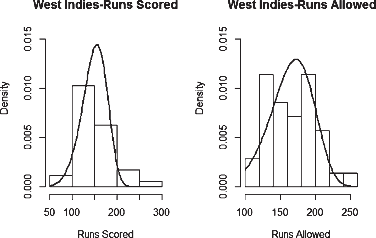
Figure 1. through Fig. 4. show some representative plots to describe the appropriateness of the Weibull fit for the observed data. The complete list of plots can be found in the appendix.
Fig. 1
Weibull Distribution Fit for Runs Scored and Runs Allowed for Australia using Least Squares Method (ODI).
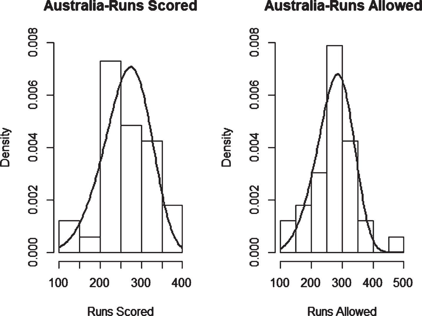
Fig. 2
Weibull Distribution Fit for Runs Scored and Runs Allowed for New Zealand using Maximum Likelihood Method (ODI).
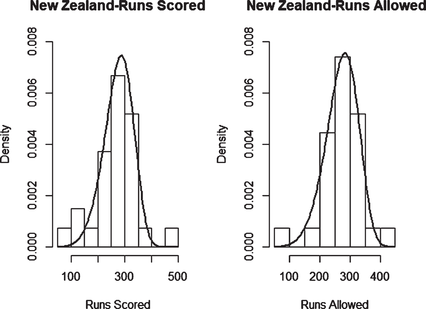
Fig. 3
Weibull Distribution Fit for Runs Scored and Runs Allowed for England using Least Squares Method (Twenty20).
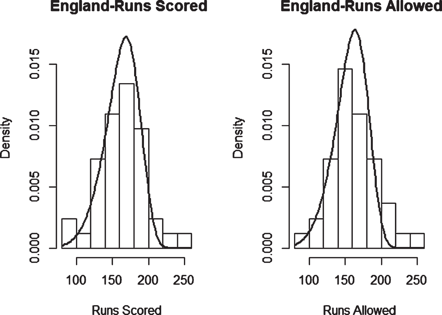
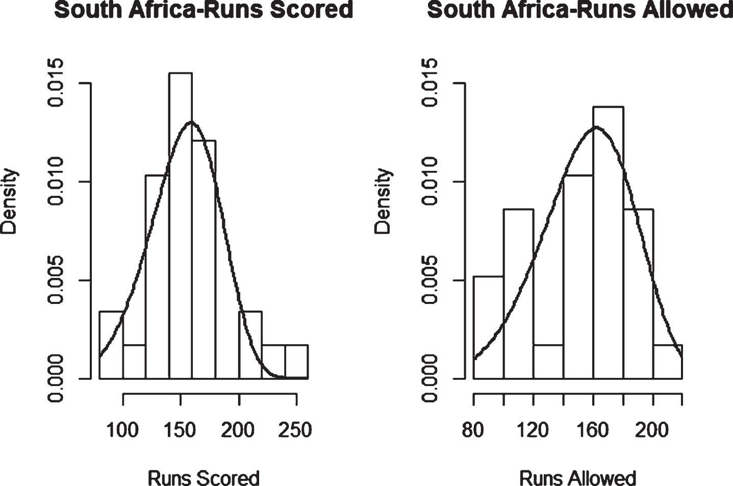
Fig. 4
Weibull Distribution Fit for Runs Scored and Runs Allowed for South Africa using Maximum Likelihood Method (Twenty20).
As can be seen from Table 10, all the p-values are above 0.05, which indicates that the use of Weibull distribution for runs scored and runs allowed is appropriate for ODI data. Table 11 shows the same for Twenty20 data, and the results are consistent, meaning that the use of Weibull distribution for runs scored and runs allowed is appropriate for Twenty20 data as well.
Table 10
Goodness of Fit – Weibull Distribution (ODI Matches -Maximum Likelihood Method)
| Team | Chi-squared RS | p-value | Chi-squared RA | p-value |
| AFG | 3.58 | 0.997 | 0.84 | 0.999 |
| AUS | 4.67 | 0.989 | 17.43 | 0.234 |
| BAN | 5.56 | 0.976 | 2.68 | 0.999 |
| ENG | 7.96 | 0.892 | 3.41 | 0.998 |
| IND | 4.65 | 0.990 | 4.50 | 0.992 |
| NZ | 11.67 | 0.633 | 7.54 | 0.912 |
| PAK | 7.11 | 0.930 | 6.19 | 0.961 |
| SA | 7.67 | 0.906 | 2.41 | 0.999 |
| SL | 3.57 | 0.998 | 5.48 | 0.978 |
| WI | 4.04 | 0.995 | 8.46 | 0.864 |
Table 11
Goodness of Fit – Weibull Distribution (Twenty20 Matches -Maximum Likelihood Method)
| Team | Chi-squared RS | p-value | Chi-squared RA | p-value |
| AFG | 5.86 | 0.923 | 1.66 | 0.999 |
| AUS | 5.40 | 0.944 | 3.36 | 0.992 |
| BAN | 4.35 | 0.976 | 6.85 | 0.867 |
| ENG | 4.40 | 0.975 | 1.35 | 0.999 |
| IND | 3.93 | 0.985 | 6.23 | 0.904 |
| NZ | 6.96 | 0.860 | 9.50 | 0.660 |
| PAK | 3.69 | 0.988 | 1.73 | 0.999 |
| SA | 0.98 | 0.999 | 4.87 | 0.962 |
| SL | 4.04 | 0.983 | 3.99 | 0.983 |
| WI | 2.03 | 0.999 | 8.25 | 0.766 |
Note that we have also investigated the goodness of fit of Weibull distribution using least squares estimates. However, the results were closely similar to those obtained using the maximum likelihood method. Therefore, tables showing the least squares results are not included here.
3.3Independence of runs scored and runs allowed
Kendall’s Tau test was applied to test the statistical independence of runs scored and runs allowed for both ODI and Twenty20 formats. This test is a nonparametric method to test the statistical independence of two random variables. A Kendall’s Tau value closer to zero is an indication of the independence of two random variables.
As seen in Table 12, runs scored and runs allowed were statistically independent for all ODI teams except Bangladesh (p-values are greater than 0.05).
Table 12
Results of Kendall’s Tau Test for ODI Cricket Matches
| Team | Z or T value | p-value | Tau Estimate |
| AFG | 7.000 | 1.000 | –0.067 |
| AUS | 1.411 | 0.158 | 0.173 |
| BAN | –2.08 | 0.038 | –0.339 |
| ENG | 1.571 | 0.116 | 0.203 |
| IND | –1.568 | 0.117 | –0.164 |
| NZ | –1.189 | 0.235 | –0.163 |
| PAK | –0.372 | 0.710 | –0.046 |
| SA | –0.633 | 0.527 | –0.079 |
| SL | 1.800 | 0.072 | 0.257 |
| WI | 0.291 | 0.771 | 0.044 |
Table 13 shows that for Twenty20 cricket, runs scored and runs allowed were statistically independent for only four of the ten teams (Afghanistan, Australia, New Zealand, and West Indies). As we see, the independence assumption is valid for the ODI data but not for the Twenty20 data. One explanation for why the assumption does not hold for the Twenty20 data while it does for ODI data is the difference in length of the two formats. Usually when the second batting team bats, it uses the first team’s score as the target. This could induce a dependency between the two scores. With the ODI, this dependency vanishes due to the longer playing time (number of overs). It might be the case that the length of the Twenty20 format does not have enough time (number of overs) to eliminate this dependency. Therefore, the results related to the Twenty20 data reported herein should be considered in light of limitations of the validity of the assumption of independence.
Table 13
Results of Kendall’s Tau test for Twenty20 Cricket Matches
| Team | Z or T value | p-value | Tau Estimate |
| AFG | 0.383 | 0.702 | 0.138 |
| AUS | 0.568 | 0.570 | 0.059 |
| BAN | 2.739 | 0.006 | 0.349 |
| ENG | 2.339 | 0.019 | 0.256 |
| IND | 3.802 | 0.000 | 0.468 |
| NZ | –0.125 | 0.901 | –0.016 |
| PAK | 3.139 | 0.002 | 0.345 |
| SA | 3.380 | 0.001 | 0.447 |
| SL | 3.036 | 0.002 | 0.333 |
| WI | 0.597 | 0.550 | 0.071 |
4Discussion and conclusion
In this study, we have shown how Bill James’ Pythagorean formula can be applied to the game of cricket. In particular, we have derived the appropriate exponent γ for the two limited-overs international cricket formats ODI and Twenty20. The maximum likelihood method has resulted in mean γ values of 4.71 for ODI matches and 6.06 for Twenty20 matches. The least squares method resulted in slightly higher values for both formats, with mean γ values 5.01 and 6.56 respectively for ODI and Twenty20. Given the desirable properties such as consistency, invariance, asymptotic normality, and relationship to the sufficient statistics, we suggest that the maximum likelihood estimators are more apposite estimators to be used in practice. In addition to this, the standard deviations of the maximum likelihood estimates of γ were lower than that of the least squares estimates for both ODI and Twenty20 formats. This concludes that the suitable γ values are 4.71 and 6.06 for ODI and Twenty20 respectively. The only comparison that can be found in the literature is the γ value 7.41, which was given by Vine (2016) for the Twenty20 cricket Big Bash League, an Australian domestic competition.
The significance of the findings of this paper is that it was based on international Twenty20 and ODI cricket matches. Note that the independence assumption is valid for the ODI data, but for the Twenty20 data, it was valid only for four teams. Therefore, the application of the method to the Twenty20 data should be done cautiously due to the limitation of the validity of the assumption of independence. It would be an excellent future study to assess the robustness of the independence assumption for the Twenty20 data. Extension of the method to ODI data and incorporation of the Duckworth-Lewis method to extrapolate the runs scored by the second batting team when that team won the match without using all the resources allocated to it are also key contributions of this paper.
As mentioned in the introduction, we have used the data from the matches played during the time period between the 2015 and 2019 Cricket World Cups with the derivation of the γ for ODI matches. Consequently, we used those estimates to predict the number of matches expected to be won by each team in the 2019 World Cup. As a comparison, we have also used the regular observed winning percentages for the given time period to predict the expected win totals (number of matches) for the world cup matches. Based on our analysis, England had the highest Pythagorean winning percentage (0.76) of the 2019 World Cup, and we would have predicted them to win the tournament, which they did. Based on our findings, the Pythagorean formula would have predicted the 2019 World Cup semifinalists to be England, India, South Africa, and New Zealand. Of these, only South Africa failed to make the semifinals, with Australia qualifying instead. We have also quantified the predictive powers of the Pythagorean winning percentage and the regular observed winning percentage by using the actual win totals and implied win totals for 2019 World Cup outcomes. In particular, we have calculated
References
1 | Rosenfeld,J.W., Adler,D., Fisher,J.I. and Morris,C. (2010) . Predicting overtime with the Pythagorean formula, Journal of Quantitative Analysis in Sports 6: (1). |
2 | Chen,J. and Li,T. (2016) . The shrinkage of the Pythagorean exponents, Journal of Sports Analytics 2: (1), 37–48. |
3 | Dayaratna,K.D. and Miller,S.J. (2012) . The Pythagorean Win-Loss formula and hockey, The Hockey Research Journal 16: (1), 193–209. |
4 | Duckworth,F.C. and LewisA.J. (1998) . A fair method for resetting the target in interrupted one-day cricket matches, Journal of the Operational Research Society 49: (3), 220–227. |
5 | Heumann,J. (2016) . An improvement to the baseball statistic Pythagorean wins, Journal of Sports Analytics 2: , 49–59. |
6 | Miller,S.J. (2006) . A derivation of the Pythagorean Win-Loss formula in baseball, The Newsletter of the SABR Statistical Analysis Committee 16: (1), 17–22. |
7 | Oliver,D. (2004) . Basketball on Paper: Rules and Tools for Performance Analysis, Brassey’s, Inc., Washington, D.C. |
8 | Perera,H.P. and Swartz,T.B. (2013) . Resources estimation in T cricket, IMA Journal of Management Mathematics 24: (3), 337–347. |
9 | Schatz,A. (2003) . Pythagorean on the gridiron, Football Outsiders. https://www.footballoutsiders.com/stat-analysis/2003/pythagoras-gridiron. |
10 | Vine,A.J. (2016) . Using Pythagorean expectation to determine luck in the KFC Big Bash League, Economic Papers 35: (3), 269–281. |
Appendices
Appendix
Fig. 5
Weibull Distribution Fit for Runs Scored and Runs Allowed for Afghanistan using Least Squares Method (ODI).
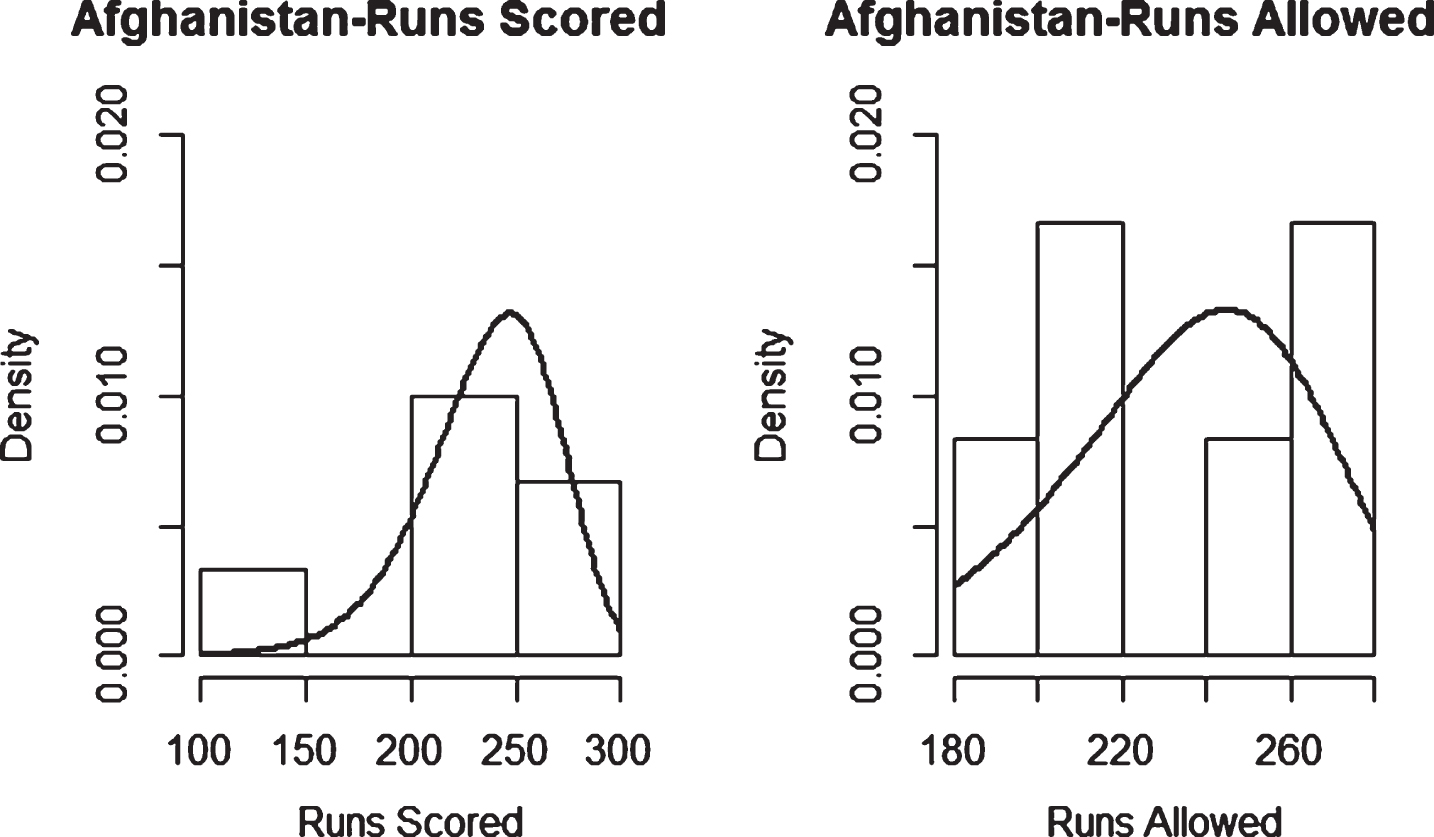
Fig. 6
Weibull Distribution Fit for Runs Scored and Runs Allowed for Afghanistan using Maximum Likelihood Method (ODI).
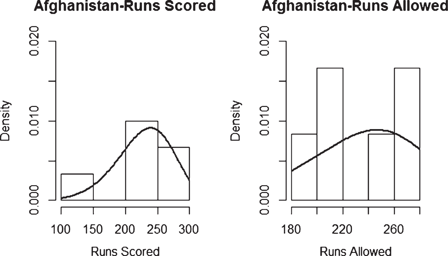
Fig. 7
Weibull Distribution Fit for Runs Scored and Runs Allowed for Australia using Maximum Likelihood Method (ODI).
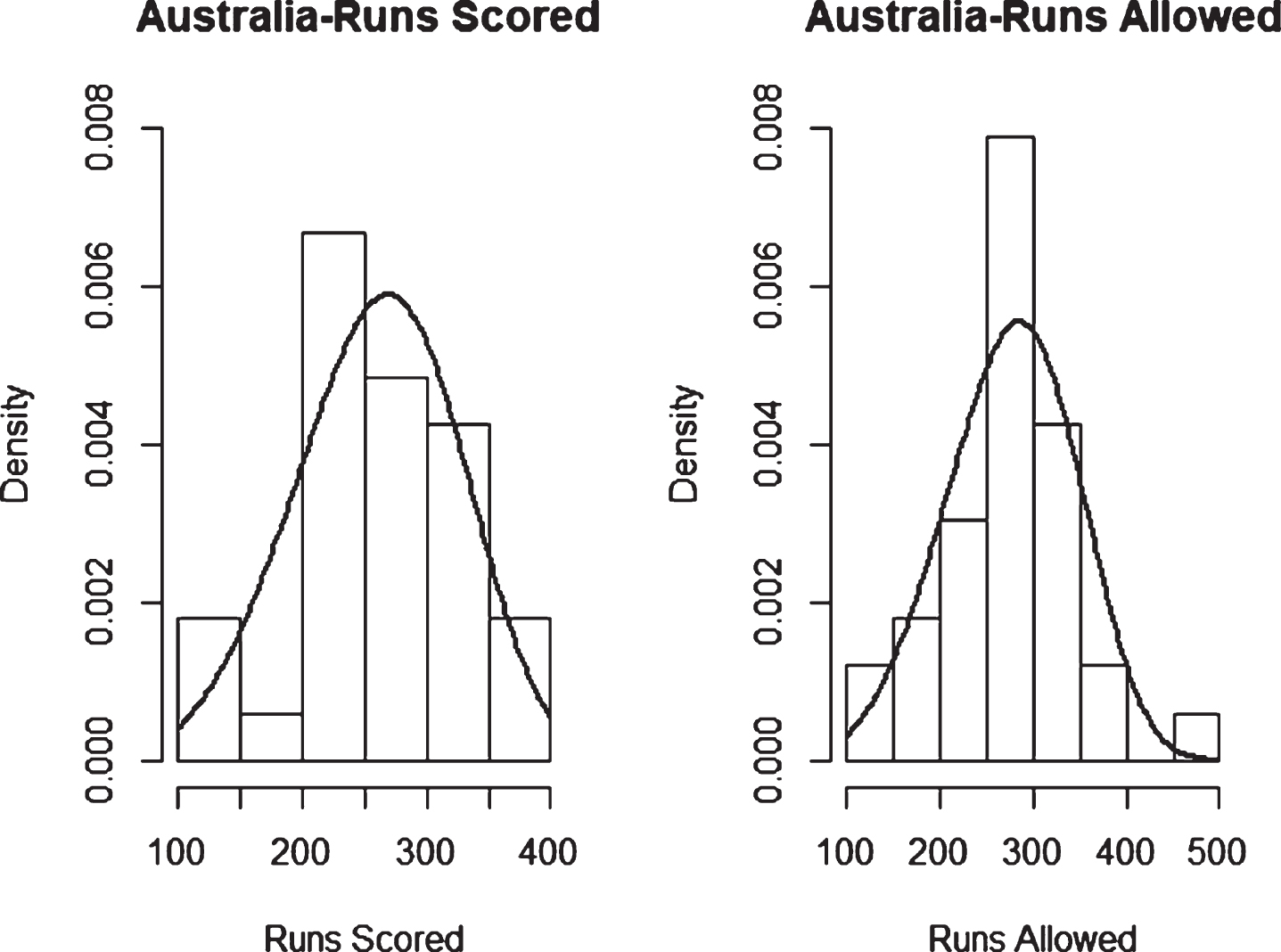
Fig. 8
Weibull Distribution Fit for Runs Scored and Runs Allowed for Bangladesh using Least Squares Method (ODI).
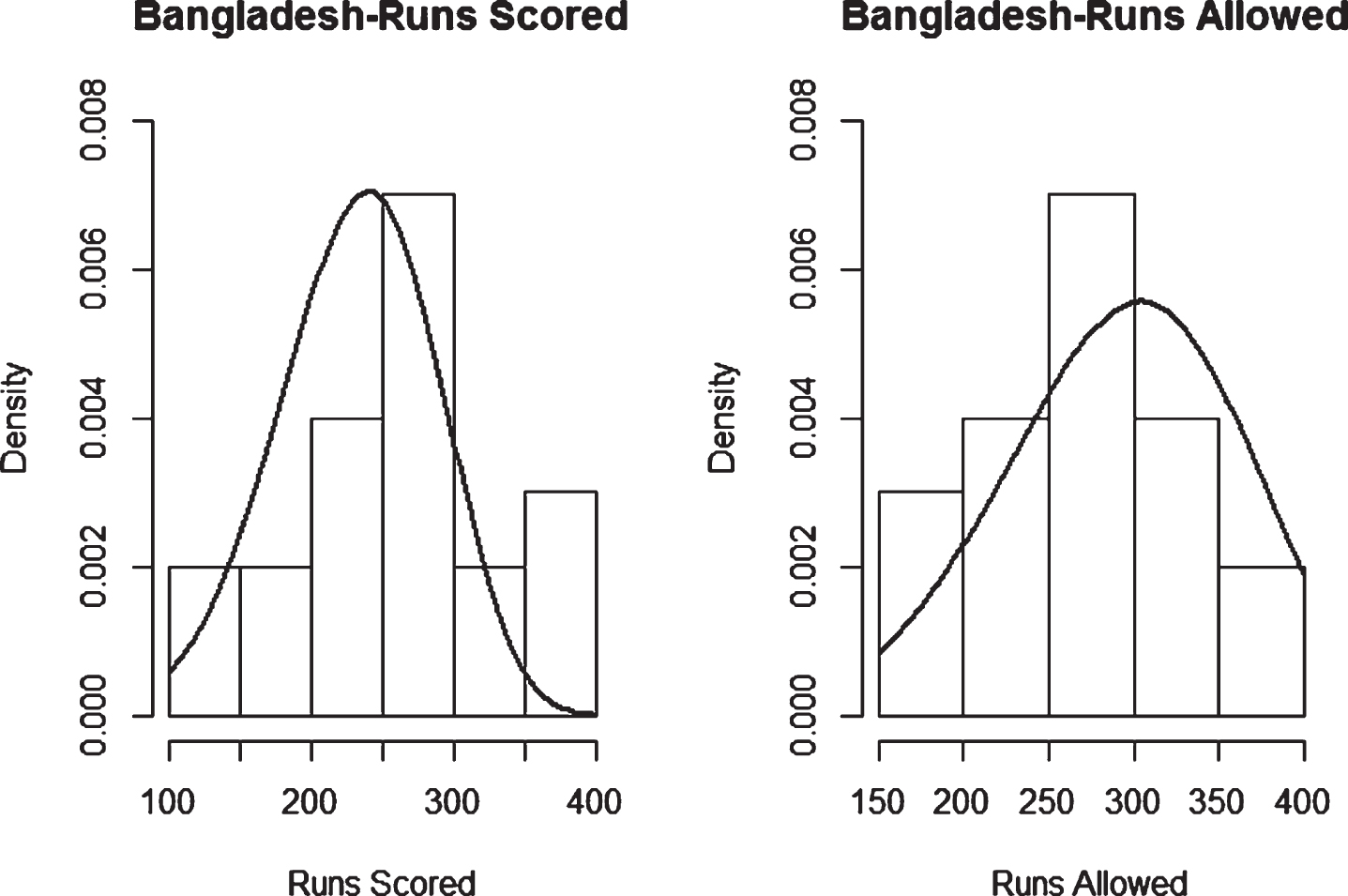
Fig. 9
Weibull Distribution Fit for Runs Scored and Runs Allowed for Bangladesh using Maximum Likelihood Method (ODI).
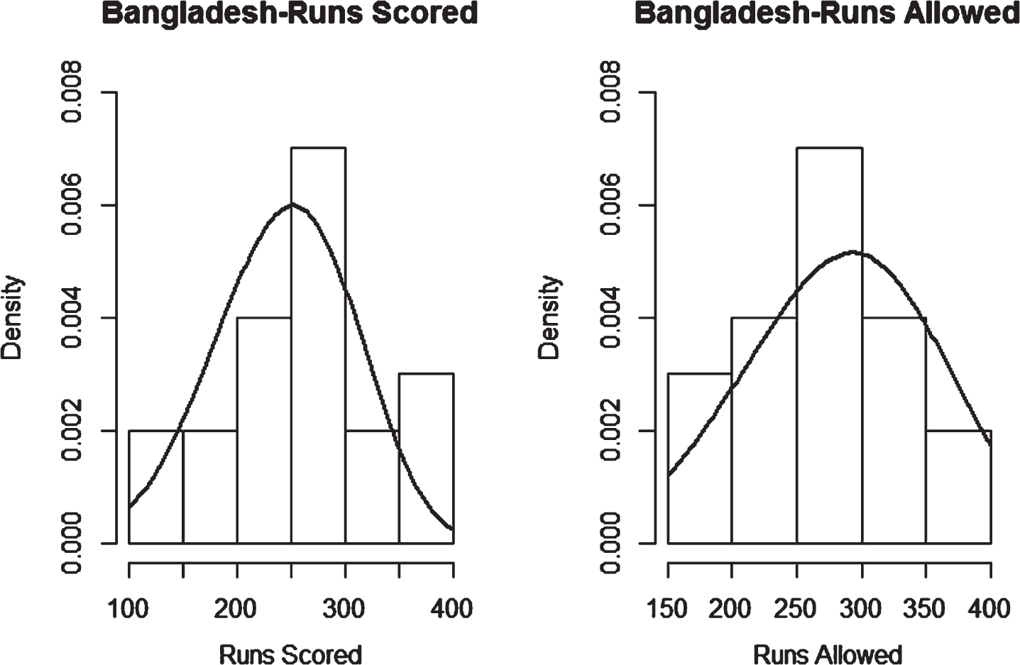
Fig. 10
Weibull Distribution Fit for Runs Scored and Runs Allowed for England using Least Squares Method (ODI).
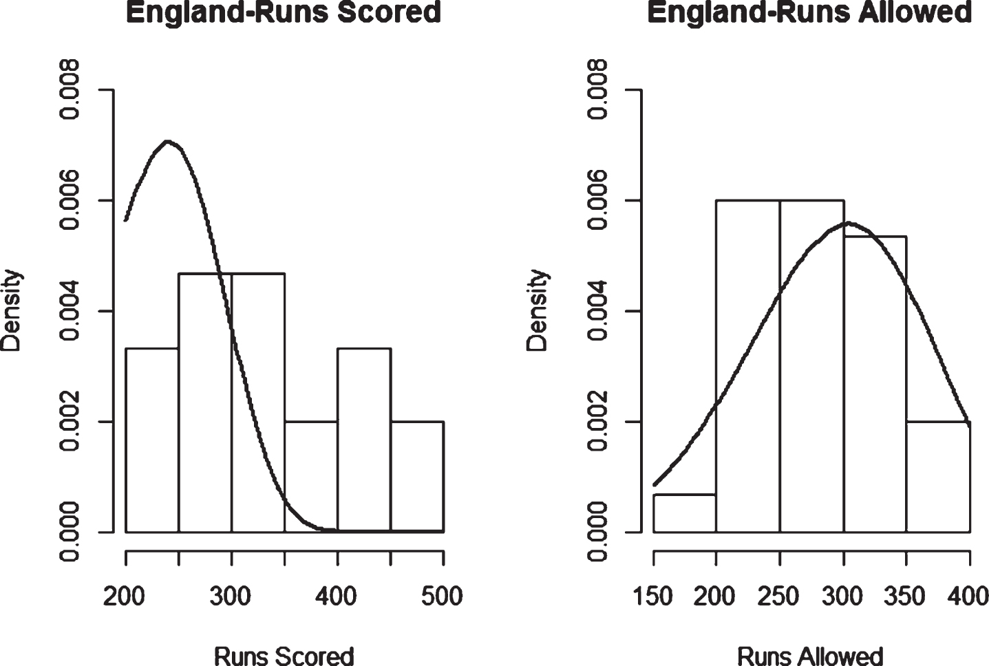
Fig. 11
Weibull Distribution Fit for Runs Scored and Runs Allowed for England using Maximum Likelihood Method (ODI).
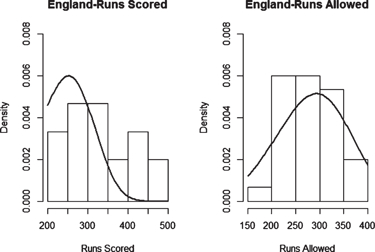
Fig. 12
Weibull Distribution Fit for Runs Scored and Runs Allowed for India using Least Squares Method (ODI).
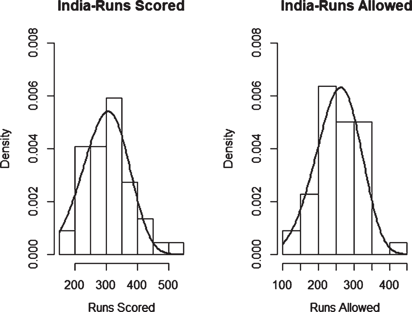
Fig. 13
Weibull Distribution Fit for Runs Scored and Runs Allowed for India using Maximum Likelihood Method (ODI).
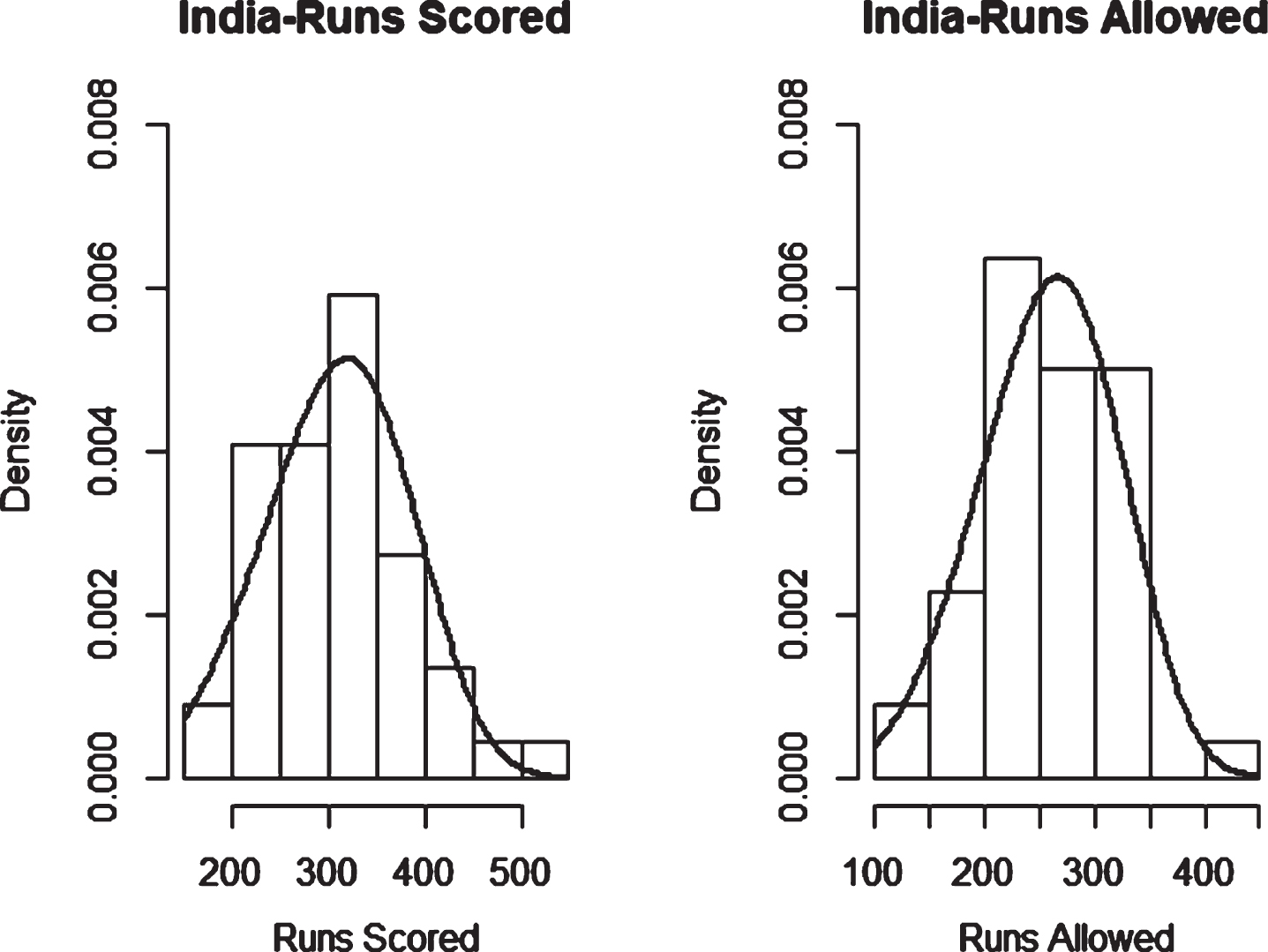
Fig. 14
Weibull Distribution Fit for Runs Scored and Runs Allowed for New Zealand using Least Squares Method (ODI).
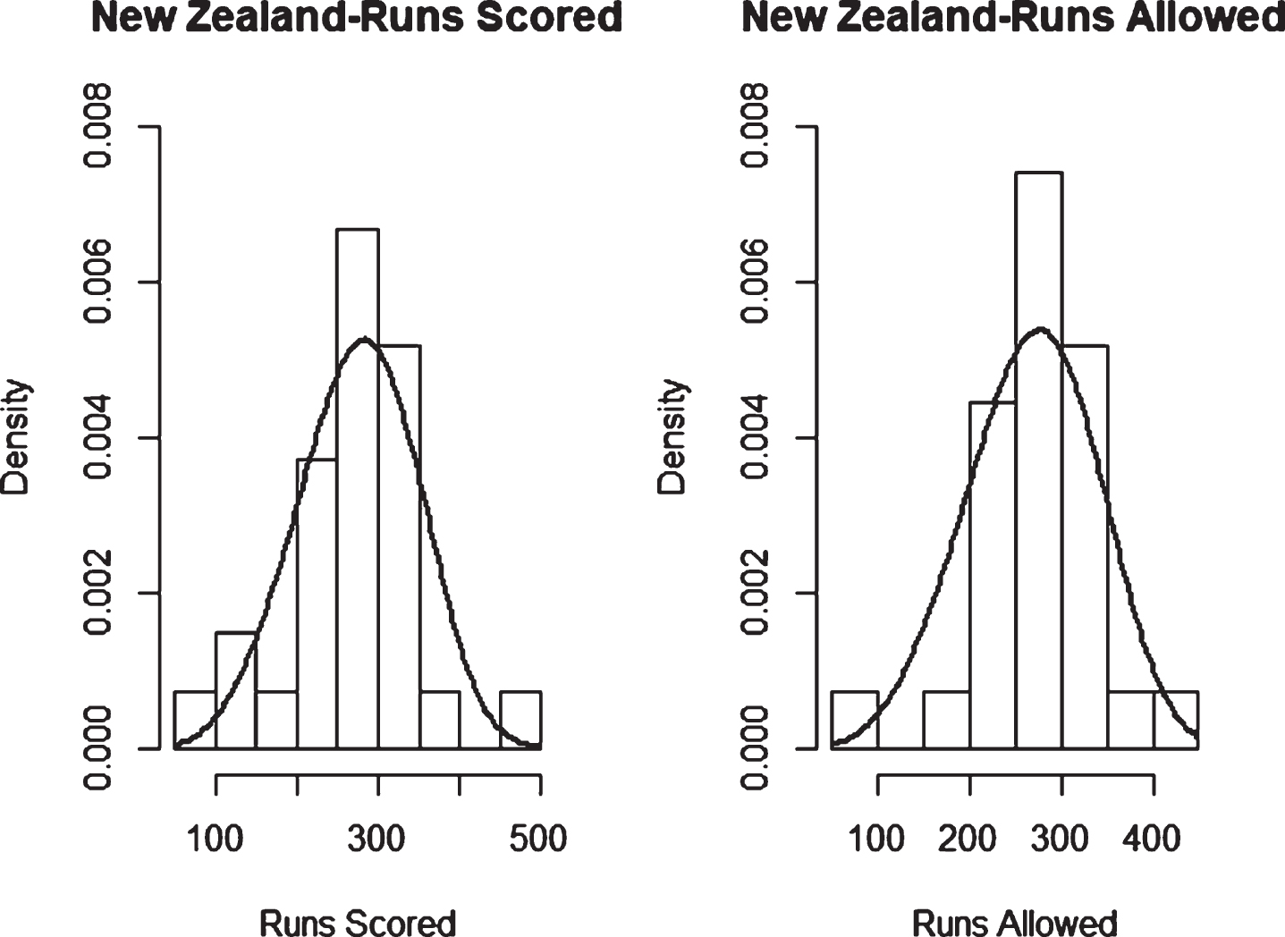
Fig. 15
Weibull Distribution Fit for Runs Scored and Runs Allowed for Pakistan using Least Squares Method (ODI).
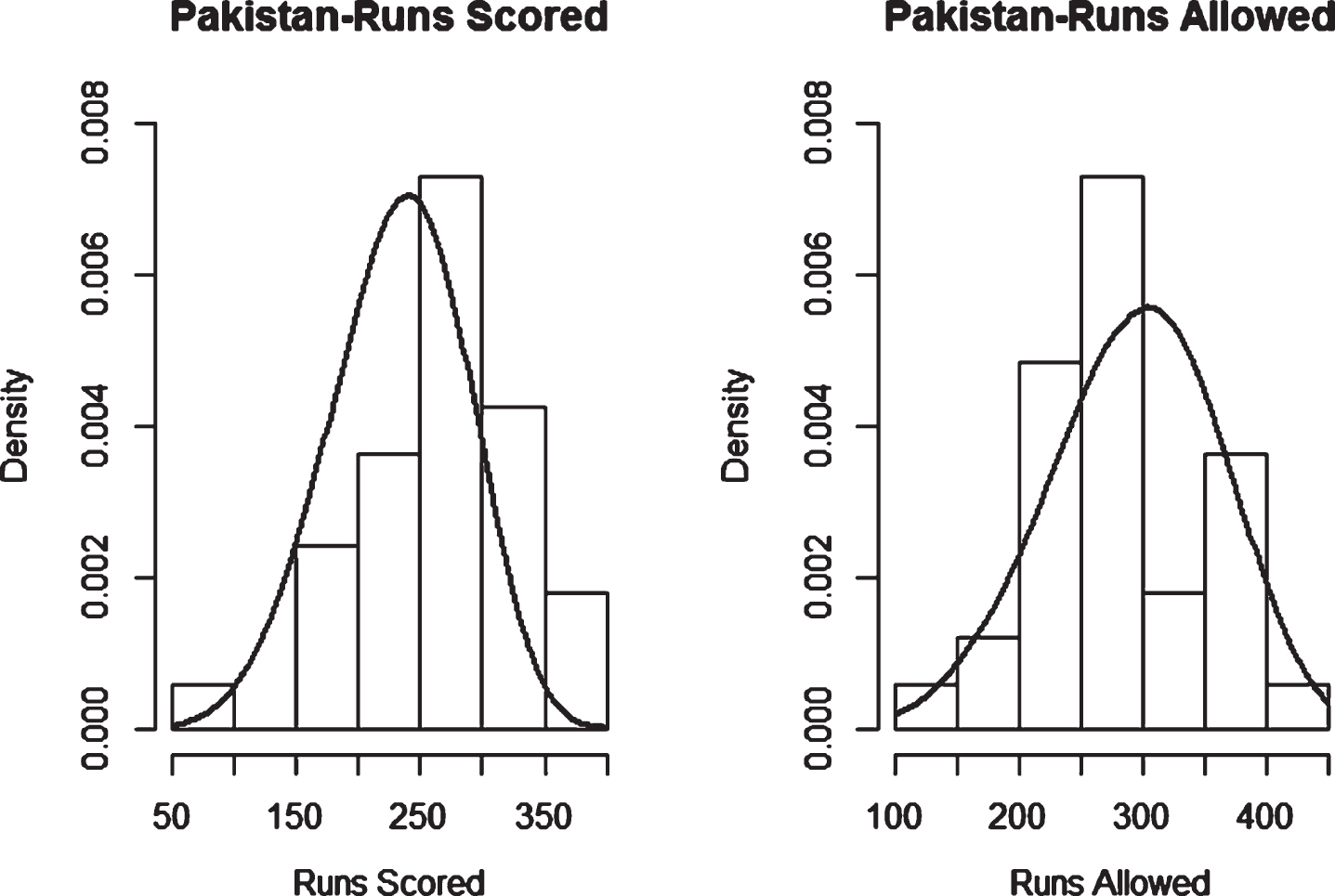
Fig. 16
Weibull Distribution Fit for Runs Scored and Runs Allowed for Pakistan using Maximum Likelihood Method (ODI).
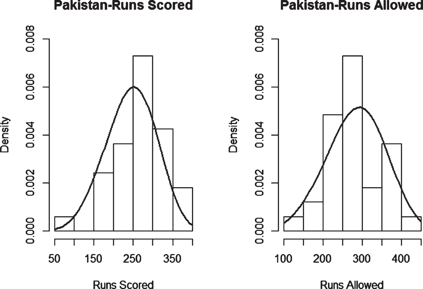
Fig. 17
Weibull Distribution Fit for Runs Scored and Runs Allowed for South Africa using Least Squares Method (ODI).
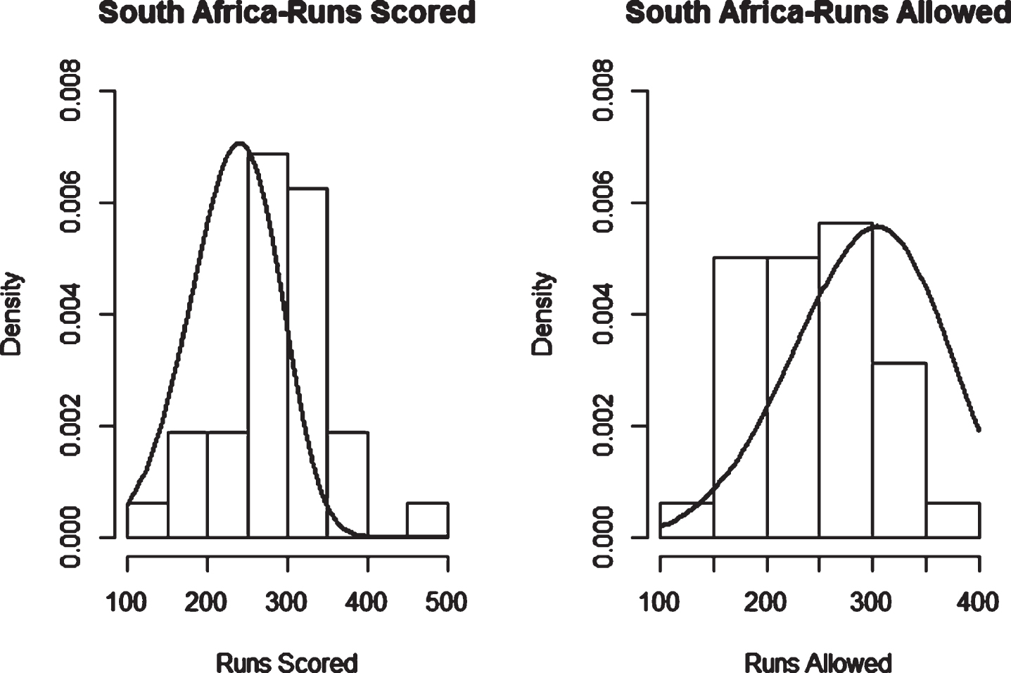
Fig. 18
Weibull Distribution Fit for Runs Scored and Runs Allowed for South Africa using Maximum Likelihood Method (ODI).
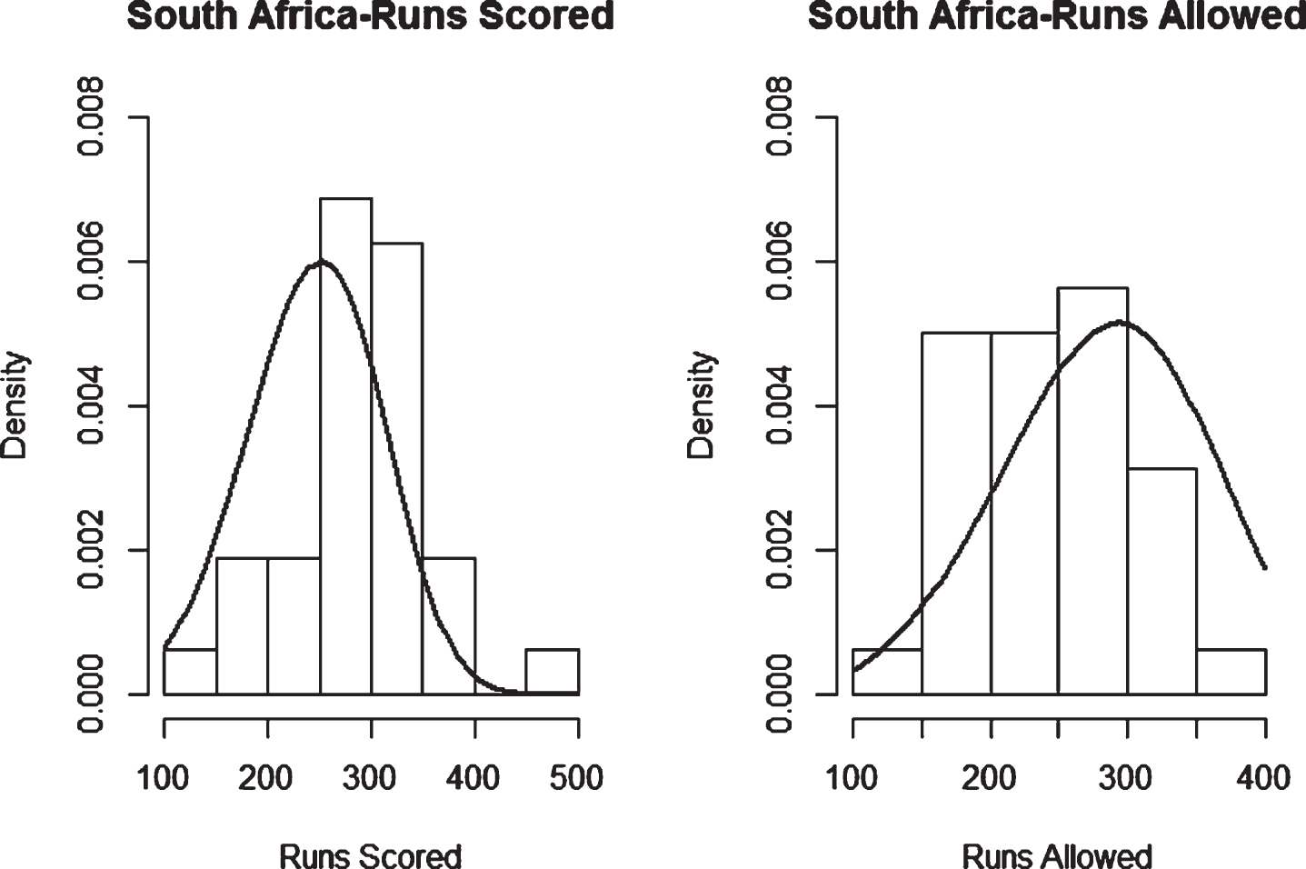
Fig. 19
Weibull Distribution Fit for Runs Scored and Runs Allowed for Sri Lanka using Least Squares Method (ODI).
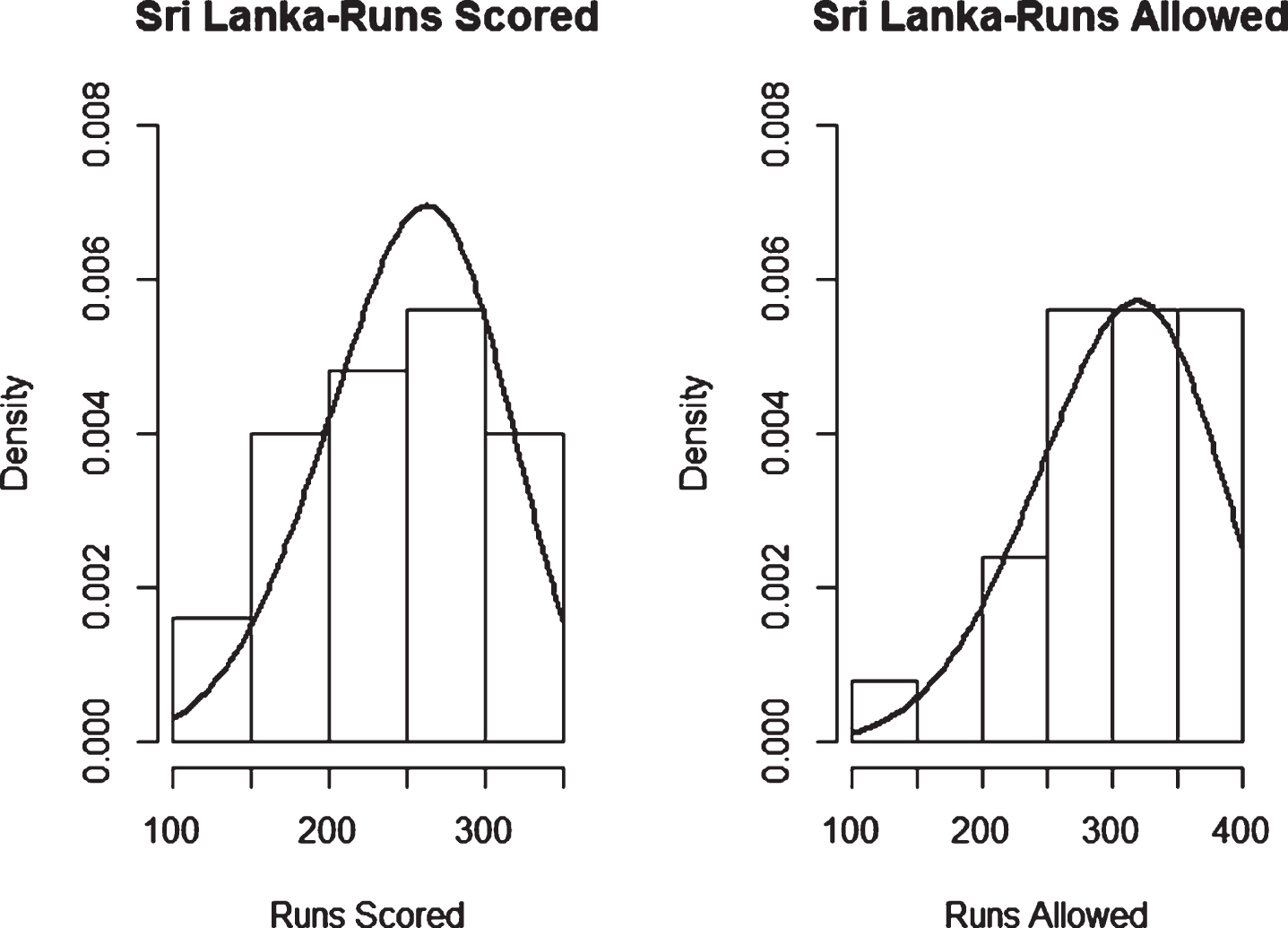
Fig. 20
Weibull Distribution Fit for Runs Scored and Runs Allowed for Sri Lanka using Maximum Likelihood Method (ODI).
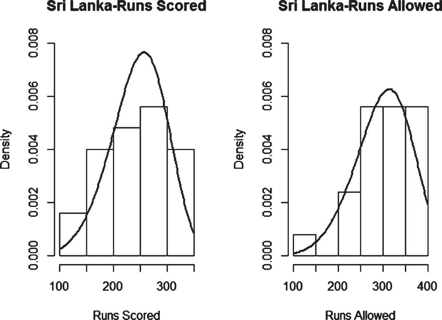
Fig. 21
Weibull Distribution Fit for Runs Scored and Runs Allowed for West Indies using Least Squares Method (ODI).
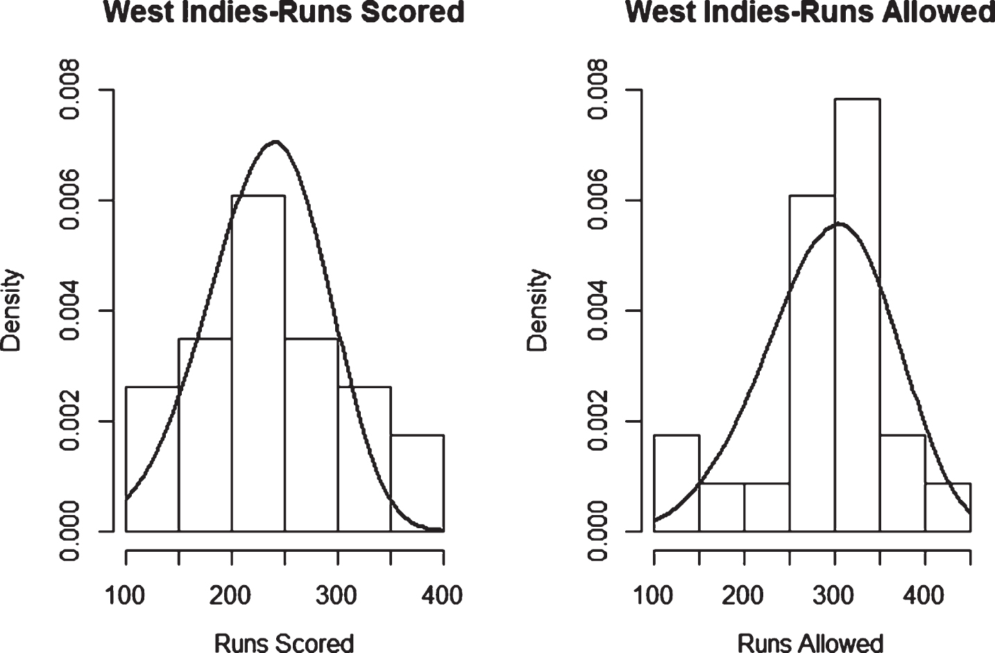
Fig. 22
Weibull Distribution Fit for Runs Scored and Runs Allowed for West Indies using Maximum Likelihood Method (ODI).
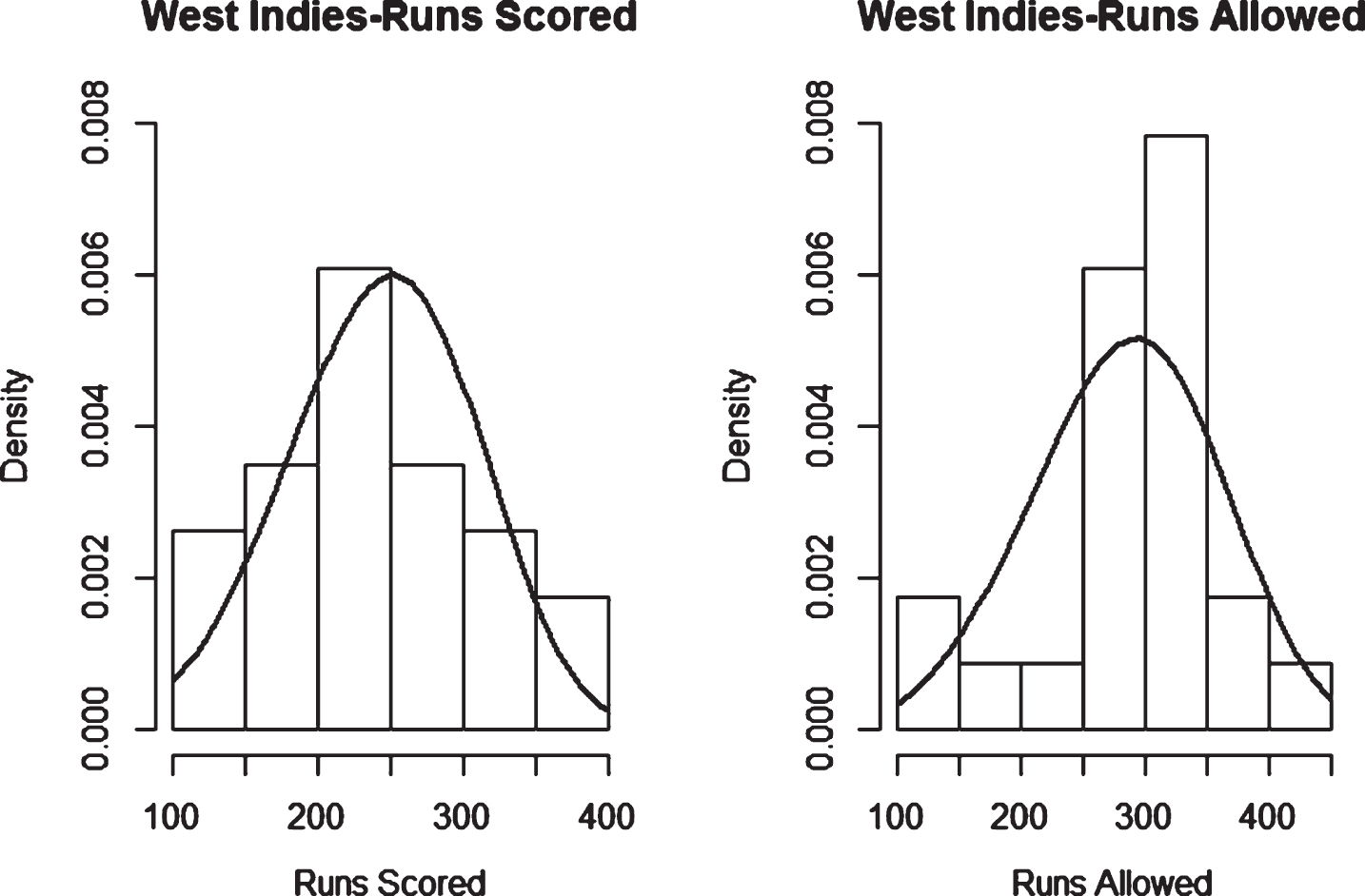
Fig. 23
Weibull Distribution Fit for Runs Scored and Runs Allowed for Afghanistan using Least Squares Method (Twenty20).

Fig. 24
Weibull Distribution Fit for Runs Scored and Runs Allowed for Afghanistan using Maximum Likelihood Method (Twenty20).
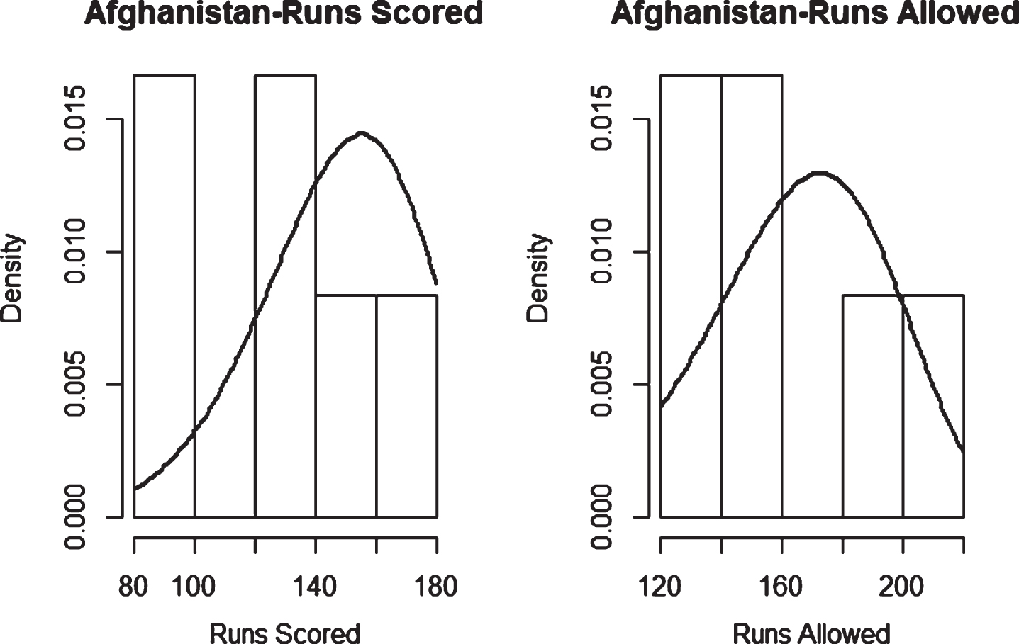
Fig. 25
Weibull Distribution Fit for Runs Scored and Runs Allowed for Australia using Least Squares Method (Twenty20).
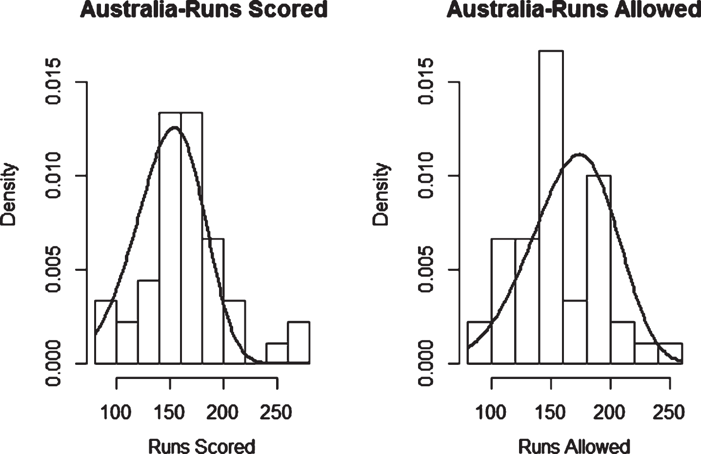
Fig. 26
Weibull Distribution Fit for Runs Scored and Runs Allowed for Australia using Maximum Likelihood Method (Twenty20).
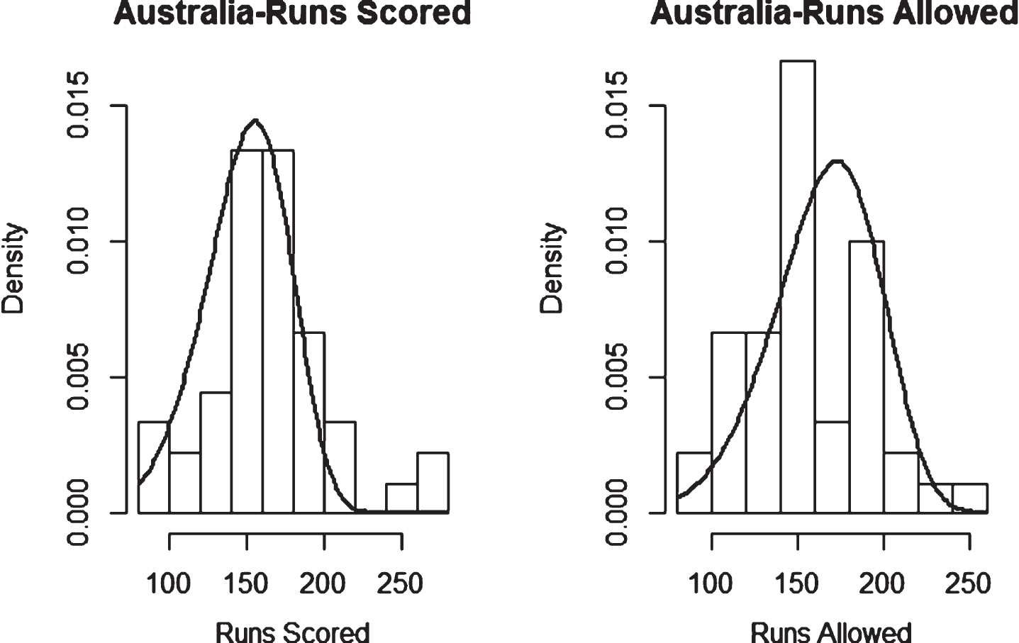
Fig. 27
Weibull Distribution Fit for Runs Scored and Runs Allowed for Bangladesh using Least Squares Method (Twenty20).
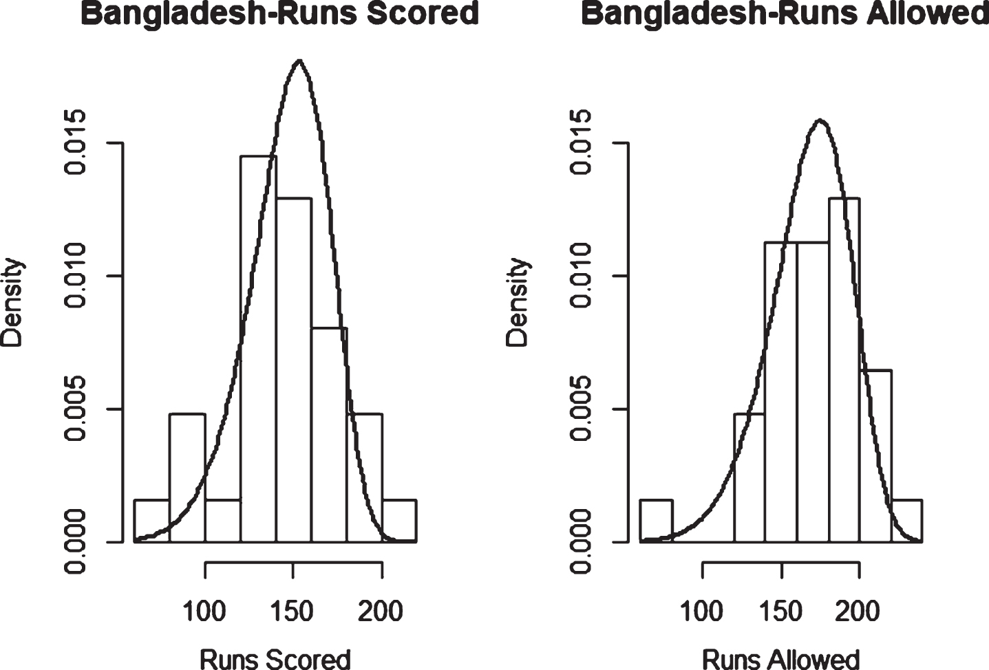
Fig. 28
Weibull Distribution Fit for Runs Scored and Runs Allowed for Bangladesh using Maximum Likelihood Method (Twenty20).
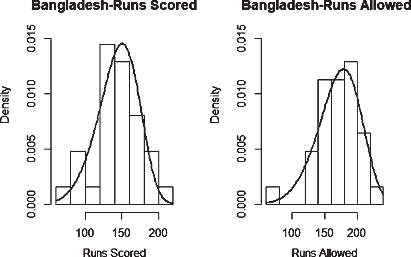
Fig. 29
Weibull Distribution Fit for Runs Scored and Runs Allowed for England using Maximum Likelihood Method (Twenty20).
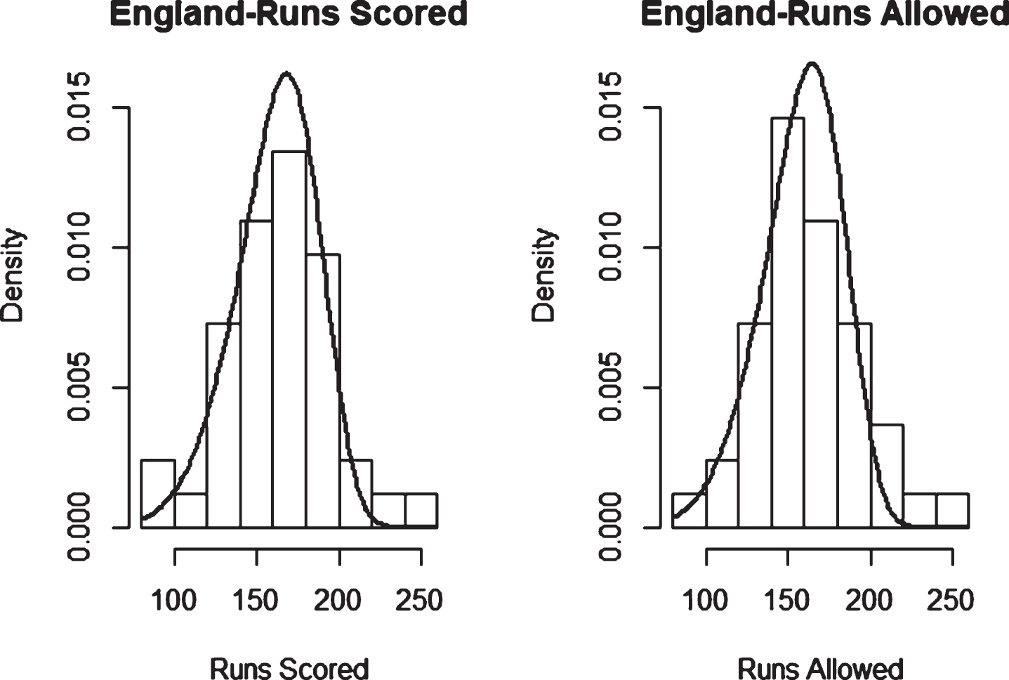
Fig. 30
Weibull Distribution Fit for Runs Scored and Runs Allowed for India using Least Squares Method (Twenty20).
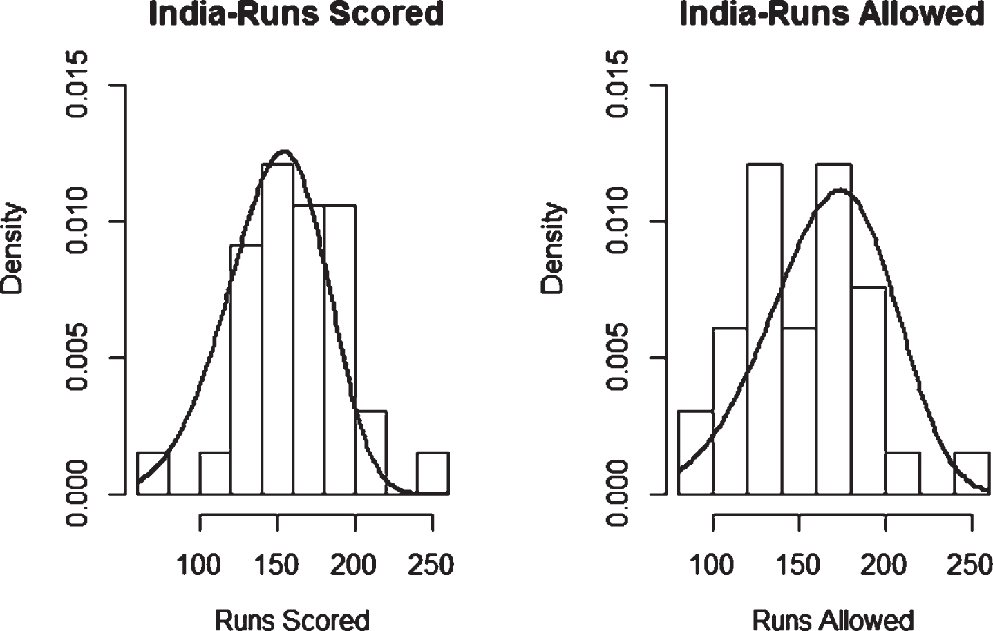
Fig. 31
Weibull Distribution Fit for Runs Scored and Runs Allowed for India using Maximum Likelihood Method (Twenty20).
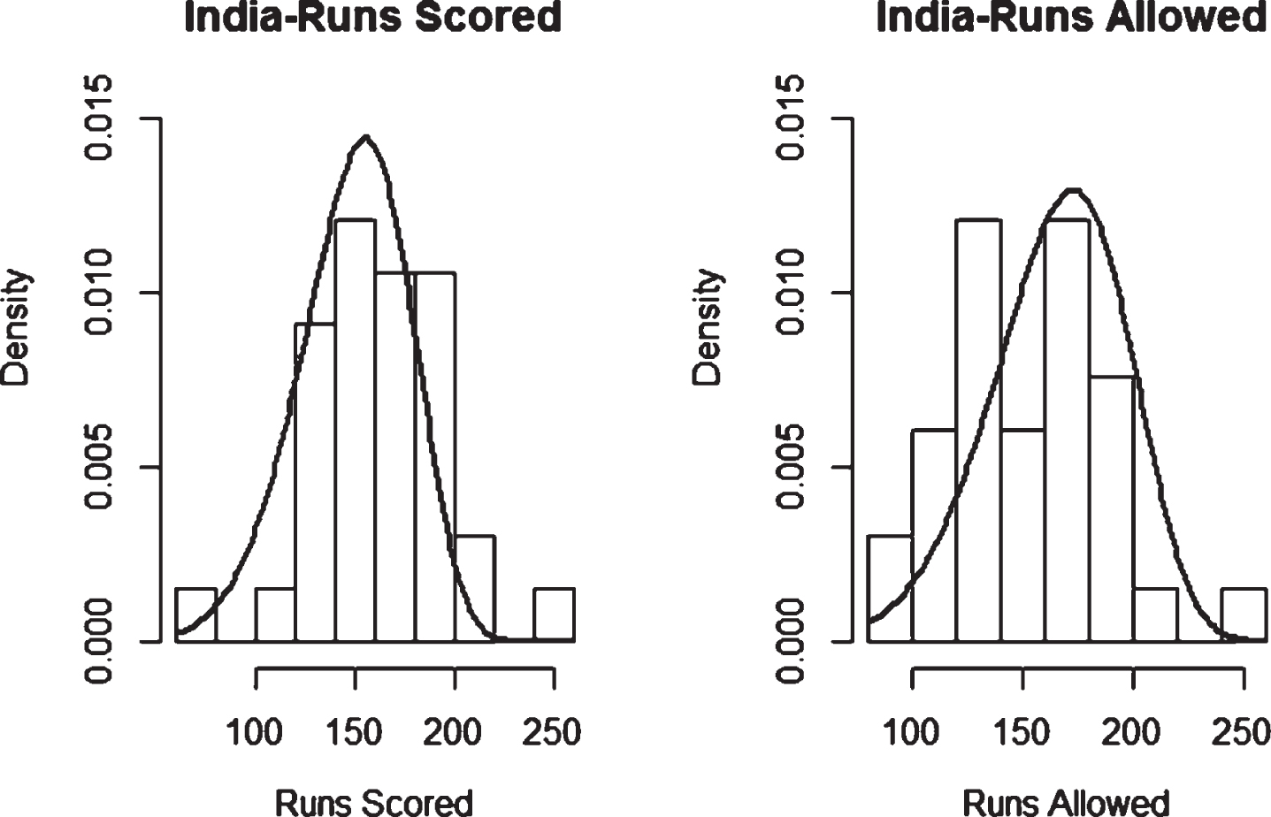
Fig. 32
Weibull Distribution Fit for Runs Scored and Runs Allowed for New Zealand using Least Squares Method (Twenty20).
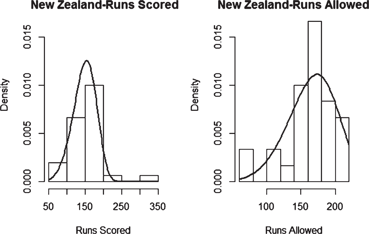
Fig. 33
Weibull Distribution Fit for Runs Scored and Runs Allowed for New Zealand using Maximum Likelihood Method (Twenty20).
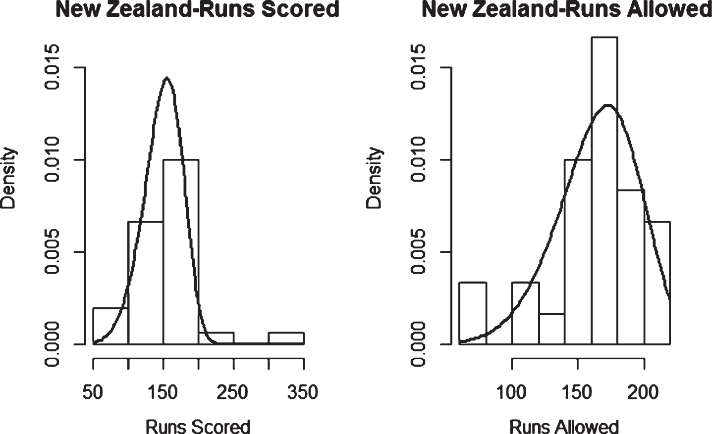
Fig. 34
Weibull Distribution Fit for Runs Scored and Runs Allowed for Pakistan using Least Squares Method (Twenty20).

Fig. 35
Weibull Distribution Fit for Runs Scored and Runs Allowed for Pakistan using Maximum Likelihood Method (Twenty20).
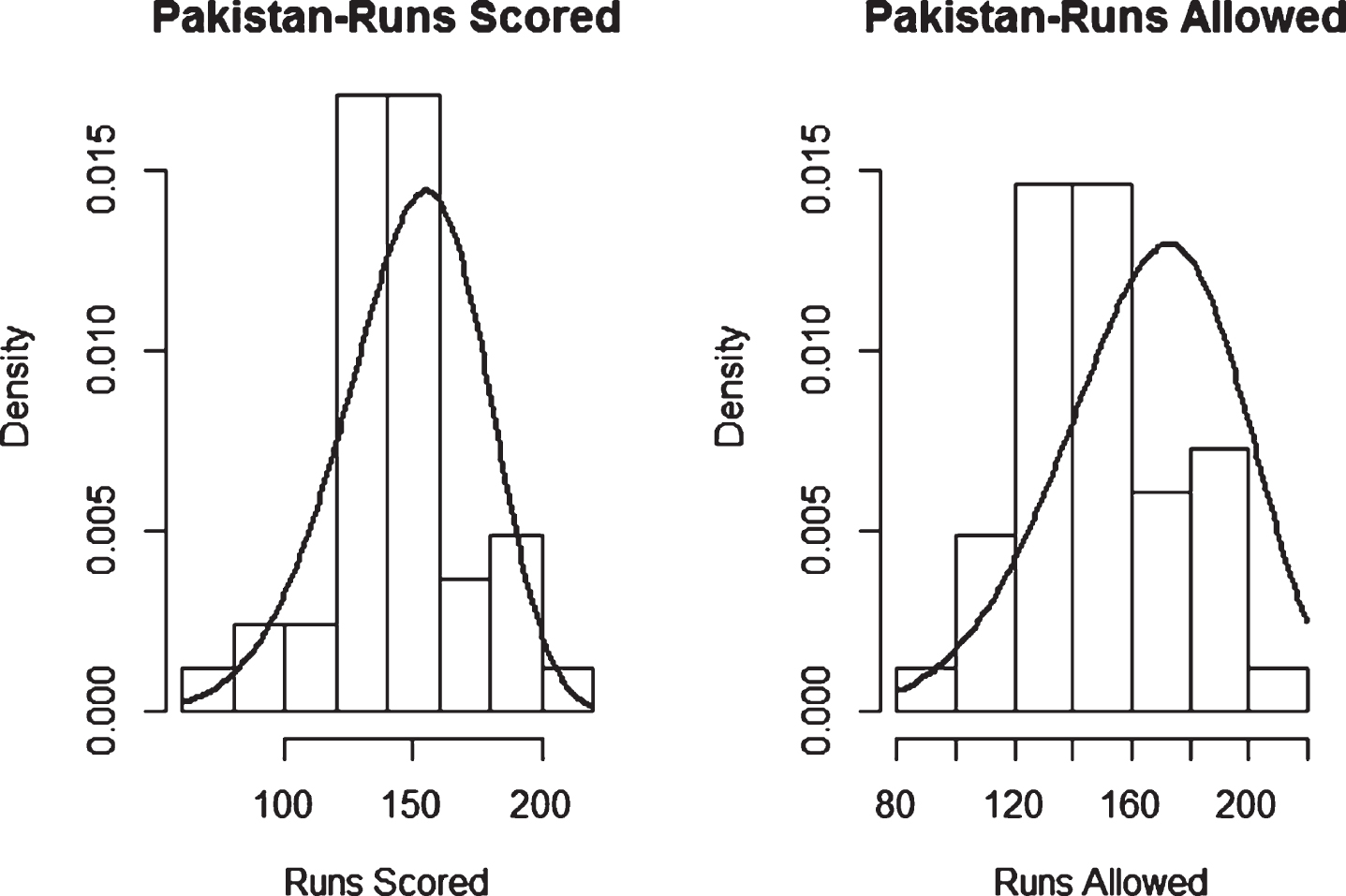
Fig. 36
Weibull Distribution Fit for Runs Scored and Runs Allowed for South Africa using Least Squares Method (Twenty20).
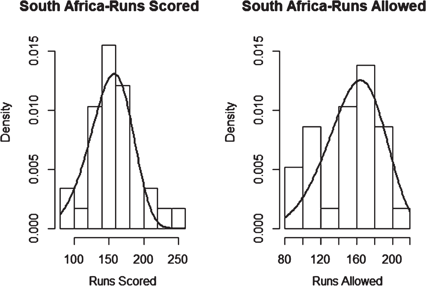
Fig. 37
Weibull Distribution Fit for Runs Scored and Runs Allowed for Sri Lanka using Least Squares Method (Twenty20).
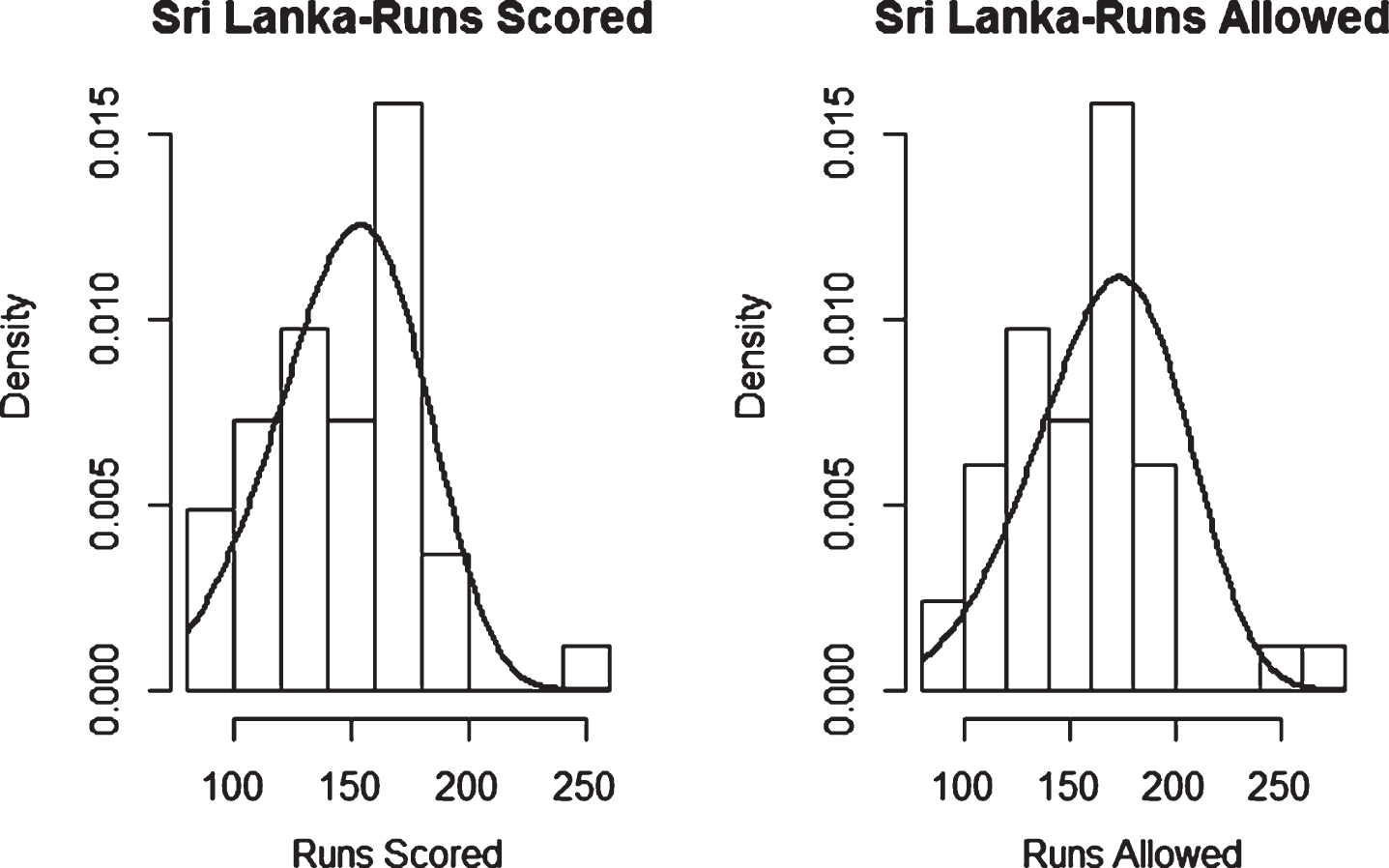
Fig. 38
Weibull Distribution Fit for Runs Scored and Runs Allowed for Sri Lanka using Maximum Likelihood Method (Twenty20).
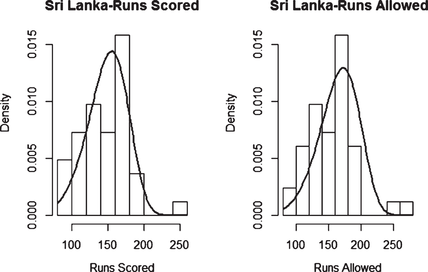
Fig. 39
Weibull Distribution Fit for Runs Scored and Runs Allowed for West Indies using Least Squares Method (Twenty20).
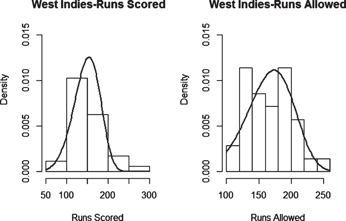
Fig. 40
Weibull Distribution Fit for Runs Scored and Runs Allowed for West Indies using Maximum Likelihood Method (Twenty20).