
Forecasting football matches by predicting match statistics
Abstract
This paper considers the use of observed and predicted match statistics as inputs to forecasts for the outcomes of football matches. It is shown that, were it possible to know the match statistics in advance, highly informative forecasts of the match outcome could be made. Whilst, in practice, match statistics are clearly never available prior to the match, this leads to a simple philosophy. If match statistics can be predicted pre-match, and if those predictions are accurate enough, it follows that informative match forecasts can be made. Two approaches to the prediction of match statistics are demonstrated: Generalised Attacking Performance (GAP) ratings and a set of ratings based on the Bivariate Poisson model which are named Bivariate Attacking (BA) ratings. It is shown that both approaches provide a suitable methodology for predicting match statistics in advance and that they are informative enough to provide information beyond that reflected in the odds. A long term and robust gambling profit is demonstrated when the forecasts are combined with two betting strategies.
1Introduction
Quantitative analysis of sports is a rapidly growing discipline with participants, coaches, owners, as well as gamblers, increasingly recognising its potential in gaining an edge over their opponents. This has naturally led to a demand for information that might allow better decisions to be made. Association football (hereafter football) is the most popular sport globally and, although, historically, the use of quantitative analysis has lagged behind that of US sports, this is slowly changing. Gambling on football matches has also grown significantly in popularity in recent decades and this has contributed to an increased demand for informative quantitative analysis.
Today, in the most popular football leagues globally, a great deal of match data are collected. Data on the location and outcome of every match event can be purchased, whilst free data are available including match statistics such as the numbers of shots, corners and fouls by each team. This creates huge potential for those able to process the data in an informative way. This paper focuses on probabilistic prediction of the outcomes of football matches, i.e. whether the match ends with a home win, a draw or an away win. A probabilistic forecast of such an event simply consists of estimated probabilities placed on each of the three possible outcomes. Statistical models can be used to incorporate information into probabilistic forecasts.
The basic philosophy of this paper is as follows. Suppose, somehow, that certain match statistics, such as the number of shots or corners achieved by each team, were available in advance of kickoff. In such a case, it would be reasonable to expect to be able to use this information to create informative forecasts and it is shown that this is the case. Obviously, in reality, this information would never be available in advance. However, if one can use statistics from past matches to predict the match statistics before the match begins, and those predictions are accurate enough, they can be used to create informative forecasts of the match outcome. The quality of the forecast is then dependent both on the importance of the match statistic itself and the accuracy of the pre-match prediction of that statistic.
In this paper, observed and predicted match statistics are used as inputs to a simple statistical model to construct probabilistic forecasts of match outcomes. First, observed match statistics in the form of the number of shots on target, shots off target and corners, are used to build forecasts and are shown to be informative. The observed match statistics are then replaced with predicted statistics calculated using (i) Generalised Attacking Performance (GAP) Ratings, a system which uses past data to estimate the number of defined measures of attacking performance a team can be expected to achieve in a given match (Wheatcroft, 2020), and (ii) Bivariate Attacking (BA) ratings which are introduced here and are a slightly modified version of the Bivariate Poisson model which has demonstrated favourable results in comparison to other parametric approaches (Ley et al. 2019). Whilst, unsurprisingly, it is found that predicted match statistics are less informative than observed statistics, they can still provide useful information for the construction of the forecasts. It is shown that a robust profit can be made by constructing forecasts based on predicted match statistics and using them alongside two different betting strategies.
For much of the history of sports prediction, rating systems in a similar vein to the GAP rating system used in this paper have played a key role. Probably the most well known is the Elo rating system which was originally designed to produce rankings for chess players but has a long history in other sports (Elo, et al. 1978). The Elo system assigns a rating to each player or team which, in combination with the rating of the opposition, is used to estimate the probability of each possible outcome. The ratings are updated after each game in which a player or team is involved. A weakness of the original Elo rating system is that it does not estimate the probability of a draw. As such, in sports such as football, in which draws are common, some additional methodology is required to estimate that probability.
Elo ratings are in widespread use in football and have been demonstrated to perform favourably with respect to other rating systems (Hvattum and Arntzen, 2010). Since 2018, Fifa has used an Elo rating system to produce its international football world rankings (Fifa, 2018). Elo ratings have also been applied to a wide range of other sports including, among others, Rugby League (Carbone et al., 2016) and video games (Suznjevic et al., 2015). The website fivethirtyeight.com produces probabilities for NFL (FiveThirtyEight, 2020a) and NBA (FiveThirtyEight, 2020b) based on Elo ratings. A limitation of the Elo rating system is that it does not account for the size of a win. This means that a team’s ranking after a match would be the same after either a narrow or convincing victory. Some authors have adapted the system to account for the margin of victory (see, for example, Lasek et al. (2013) and Sullivan and Cronin (2016)).
The original Elo rating system assigns a single rating to each participating team or player, reflecting its overall ability. This does not directly allow for a distinction between the performance of a team in its home or away matches. Typically, some adjustment to the estimated probabilities is made to account for home advantage. Other rating systems distinguish between home and away performances. One system that does this is the pi-rating system in which a separate home and away rating is assigned to each team (Constantinou and Fenton, 2013). The pi-rating system also takes into account the winning margin of each team, but this is tapered such that the impact of additional goals on top of already large winning margins is lower than that of goals in close matches.
The GAP rating system, introduced in Wheatcroft (2020) and used in this paper, differs from both the Elo rating and the pi-rating systems in that, rather than producing a single rating, each team is assigned a separate attacking and defensive rating both for its home and away matches. This results in a total of 4 ratings per team. The approach of assigning attacking and defensive ratings has been taken by a large number of authors. An early example is Maher (1982) who assigned fixed ratings to each team and combined them with a Poisson model to estimate the number of goals scored. They did not use their ratings to estimate match probabilities but Dixon and Coles (1997) did so using a similar approach. Combined with a value betting strategy, they were able to demonstrate a significant profit for matches with a large discrepancy between the estimated probabilities and the probabilities implied by the odds. Dixon and Pope (2004) modified the Dixon and Coles model and were able to demonstrate a profit using a wider range of published bookmaker odds. Rue and Salvesen (2000) defined a Bayesian model for attacking and defensive ratings, allowing them to vary over time. Other examples of systems that use attacking and defensive ratings can be found in Karlis and Ntzoufras (2003), Lee (1997) and Baker and McHale (2015). Ley et al. (2019) compared ten different parametric models (with the parameters estimated using maximum likelihood) and found the Bivariate Poisson model to give the most favourable results. Koopman and Lit (2015) used a Bivariate Poisson model alongside a Bayesian approach to demonstrate a profitable betting strategy.
The use of rating systems naturally leads to the question of how to translate them into probabilistic forecasts. One of two approaches is generally taken. The first is to model the number of goals scored by each team using Poisson or Negative Binomial regression with the ratings of each team used as predictor variables. These are then used to estimate match probabilities. The second approach is to predict the probability of each match outcome directly using methods such as logistic regression. There is little evidence to suggest a major difference in the performance of the two approaches (Goddard, 2005). In this paper, the latter approach is taken, specifically in the form of ordinal logistic regression.
The idea that match statistics might be more informative than goals in terms of making match predictions has become more widespread in recent years. The rationale behind this view is that, since it is difficult to score a goal and luck often plays an important role, the number of goals scored by each team might be a poor indicator of the events of the match. It was shown by Wheatcroft (2020) that, in the over/under 2.5 goals market, the number of shots and corners provide a better basis for probabilistic forecasting than goals themselves. Related to this is the concept of ‘expected goals’ which is playing a more and more important role in football analysis. The idea is that the quality of a shot can be measured in terms of its likelihood of success. The expected goals from a particular shot corresponds to the number of goals one would ‘expect’ to score by taking that shot. The number of expected goals by each team in a match then gives an indication of how the match played out in terms of efforts at goal. Several academic papers have focused on the construction of expected goals models that take into account the location and nature of a shot (Eggels, 2016; Rathke, 2017).
This paper is organised as follows. In section 2, background information is given on betting odds and the data set used in this paper. The Bivariate Poisson model, which is used for comparison purposes in the results section and forms the basis of the Bivariate Attacking (BA) rating system is also described. In section 3, the GAP and BA rating systems are described along with the approach used for constructing forecasts of match outcomes. The two betting strategies used in the results section are also described. In section 4, the accuracy of predicted match statistics in terms of how close they get to observed statistics under the GAP and BA rating systems is compared. Match forecasts formed using different combinations of observed and predicted statistics are then compared using model selection techniques. Next, the performance of forecasts formed using combinations of predicted statistics is compared. Finally, the profitability of two betting strategies is compared when used alongside forecasts formed using different combinations of predicted match statistics. Section 6 is used for discussion.
2Background
2.1Betting odds
In this paper, betting odds are used both as potential inputs to models and as a tool with which to demonstrate profit making opportunities. Decimal, or ‘European Style’, betting odds are considered throughout. Decimal odds simply represent the number by which the gambler’s stake is multiplied in the event of success. For example, if the decimal odds are 2, a £ 10 bet on said event would result in a return of 2 × £10 = £20.
Another useful concept is that of the ‘odds implied’ probability. Let the odds for the i-th outcome of an event be Oi. The odds implied probability is simply defined as the multiplicative inverse, i.e.
(1)
2.2Data
This paper makes use of the large repository of data available at www.football-data.co.uk, which supplies free match-by-match data for 22 European Leagues. For each match, statistics are given including, among others, the number of shots, shots on target, corners, fouls and yellow cards. Odds data from multiple bookmakers are also given for the match outcome market, the over/under 2.5 goal market and the Asian Handicap match outcome market. For some leagues, match statistics are available from the 2000/2001 season onwards. For others, these are available for later seasons. Therefore, since the focus of this paper is forecasting using match statistics, only matches from the 2000/2001 season onwards are considered. The data used in this paper are summarised in Table 1 in which, for each league, the total number of matches since 2000/2001, the number of matches in which shots and corner data are available and the number of these excluding a ‘burn-in’ period for each season are shown. The meaning of the ‘burn-in’ period is explained in more detail in section 2 but simply omits the first six matches of the season played by the home team. All leagues include data up to and including the end of the 2018/19 season.
Table 1
Data used in this paper
| League | No. matches | Match data available | Excluding burn-in |
| Belgian Jupiler League | 5090 | 480 | 384 |
| English Premier League | 9120 | 7220 | 5759 |
| English Championship | 13248 | 10484 | 8641 |
| English League One | 13223 | 10460 | 8608 |
| English League Two | 13223 | 10459 | 8613 |
| English National League | 7040 | 5352 | 4642 |
| French Ligue 1 | 8718 | 4907 | 4126 |
| French Ligue 2 | 7220 | 760 | 639 |
| German Bundesliga | 7316 | 5480 | 3502 |
| German 2.Bundesliga | 5670 | 1057 | 753 |
| Greek Super League | 6470 | 477 | 381 |
| Italian Serie A | 8424 | 5275 | 4439 |
| Italian Serie B | 8502 | 803 | 680 |
| Netherlands Eredivisie | 5814 | 612 | 504 |
| Portugese Primeira Liga | 5286 | 612 | 504 |
| Scottish Premier League | 5208 | 4305 | 3427 |
| Scottish Championship | 3334 | 524 | 297 |
| Scottish League One | 3335 | 527 | 298 |
| Scottish League Two | 3328 | 525 | 297 |
| Spanish Primera Liga | 8330 | 5290 | 4449 |
| Spanish Segunda Division | 8757 | 903 | 771 |
| Turkish Super lig | 5779 | 612 | 504 |
| Total | 162435 | 77124 | 62218 |
2.3Bivariate poisson model
Poisson models are forecasting models that use the Poisson distribution to model the number of goals scored by each team in a football match. Whilst many variants of the Poisson model have been proposed, in this paper, we consider the Bivariate Poisson model proposed by Ley et al. (2019), who compared it with nine other models and found it to achieve the most favourable forecast performance (according to the ranked probability score).
The aim of a Poisson model is to estimate the Poisson parameter for each team, which can then be used to determine a forecast probability for each outcome of a match. Whilst Poisson models typically make the assumption that the number of goals scored by each team in a match is independent, there is some evidence that this is not the case. The Bivariate Poisson includes an additional parameter that removes this assumption.
In the context of this paper, the Bivariate Poisson model has two purposes. Firstly, since it has been shown to perform favourably with respect to a number of other models, it provides a powerful benchmark for comparison in section 5.3. Secondly, it provides the basis for the Bivariate Attacking (BA) rating system described in section 3.1.2.
Let Gi,m and Gj,m be random variables for the number of goals scored in the m-th match by teams i and j, respectively, where team i is at home and team j is away. In a match between the two teams, a Poisson model can be written as
(2)
The Bivariate Poisson model is an extension of another model, also described by Ley et al. (2019), called the Independent Poisson model and it is useful to define this first. The Independent Poisson Model parametrises the Poisson parameters for a home team i against an away team j as λi,m = exp (c + (ri + h) - rj) and λj,m = exp (c + rj - (ri + h)), respectively, where c is a constant parameter, h is a home advantage parameter and r1, . . . , rT are strength parameters for each team.
The Bivariate Poisson model closely resembles the independent model but introduces an extra parameter to account for potential dependency between the number of goals scored by each team. Under the Bivariate Poisson model, the joint distribution for the number of goals in a match between teams i and j is given by
(3)
Both the Independent and Bivariate Poisson models are parametric models in which the parameters are estimated using maximum likelihood. However, in both cases, a slight adjustment is made to the likelihood function such that matches that happened more recently are given more weight than those that happened longer ago. To do this, the weight placed on match m is given by
(4)
(5)
Performing maximum likelihood estimation with a large number of parameters is, in general, difficult and there is a risk of falling into local optima. We follow the approach used by Ley et al. (2019) who use the Broyden-Fletcher-Goldfarb-Shanno (BFGS) algorithm, a quasi-Newton method known for its robust properties, implemented with the ‘fmincon’ function in Matlab. Strictly positive parameters are initialised at one and each of the other parameters is initialised at zero. The sum of the team ratings r1, . . . , rT is constrained to zero.
A convenient property of the Poisson model is that the difference between two Poisson distributions follows a Skellam distribution and therefore match outcome probabilities can be estimated from the Poisson parameters for each team. For more details, see Karlis and Ntzoufras (2009).
3Methodology
3.1Ratings systems
In this paper, two different approaches are used to produce predictions for the number of goals, shots on target, shots off target and corners achieved by each team in a given football match. Each approach is described below.
3.1.1GAP ratings
The Generalised Attacking Performance (GAP) rating system, introduced by Wheatcroft (2020), is a rating system for assessing the attacking and defensive strength of a sports team with relation to a particular measure of attacking performance such as the number of shots or corners in football. For a particular given measure of attacking performance, each team in a league is given an attacking and a defensive rating, both for its home and away matches. An attacking GAP rating can be interpreted as an estimate of the number of defined attacking plays the team can be expected to achieve against an average team in the league, whilst its defensive rating can be interpreted as an estimate of the number of attacking plays it can be expected to concede against an average team. The ratings for each team are updated each time it plays a match. The GAP ratings of the i-th team in a league who have played k matches are denoted as follows:
The ratings are updated as follows. Consider a match in which the i-th team in the league is at home to the j-th team. The i-th team have played k1 previous matches and the j-th team k2. Let Si,k1 and Sj,k2 be the number of defined attacking plays by teams i and j in the match (note in many cases, both teams will have played the same number of matches and k1 and k2 will be equal). The GAP ratings for the i-th team (the home team) are updated in the following way
(6)
The GAP ratings for the j-th team (the away team) are updated as follows:
(7)
where λ > 0, 0 < ϕ1 < 1 and 0 < ϕ2 < 1 are parameters to be estimated. Here, λ determines the overall influence of a match on the ratings of each team. The parameter ϕ1 governs how the adjustments are spread over the home and away ratings of the i-th team (the home team), whilst ϕ2 governs how the adjustments are spread over the home and away ratings of the j-th team (the away team). After any given match, a home team is said to have outperformed expectations in an attacking sense if its attacking performance is higher than the mean of its attacking rating and the opposition’s defensive rating. In this case, its home attacking rating is increased (or decreased, if its attacking performance is lower than expected). If the parameter ϕ1 > 0, a team’s away ratings will be impacted by a home match, whilst a team’s home ratings will be impacted by an away match if ϕ2 > 0.
In this paper, GAP ratings are used to estimate the attacking performance of each team. For a match involving the i-th team at home to the j-th team, where the teams have played k1 and k2 previous matches in that season, respectively, the predicted numbers of defined attacking plays for the home and away teams are given by
(8)
The predicted number of attacking plays by the home team is therefore the average of the home team’s home attacking rating and the away team’s away defensive rating whilst the predicted number of attacking plays by the away team is given by the average of the away team’s away attacking rating and the home team’s home defensive rating. The predicted difference in the number of defined attacking plays made by the two teams is given by
GAP ratings are determined by three parameters which are estimated by minimising the mean absolute error between the estimated number of attacking plays and the observed number. The function to be minimised is therefore
(9)
In this paper, optimisation is performed using the fminsearch function in Matlab which implements the Nelder-Mead simplex algorithm. The small number of parameters required to be optimised makes the risk of falling into local minima small.
Note that the approach to parameter estimation in this paper, in which the parameters are based purely on the prediction accuracy of the GAP ratings with relation to the observed match statistics, differs from the approach taken in Wheatcroft (2020), in which the parameters are optimised with respect to the performance of the probabilistic forecasts for which the ratings are predictor variables (in that paper, the forecasts predict the probability that the total number of goals will exceed 2.5). Whilst a similar approach could be taken here, our chosen approach is selected to simplify the forecasting process and allow us to use as predictor variables GAP ratings based on multiple measures of attacking performance. For example, this allows for both predicted shots on target and predicted corners to be used as predictor variables without requiring simultaneous optimisation of the GAP rating parameters.
3.1.2Bivariate attacking ratings
We present an alternative approach to the GAP rating system for predicting match statistics which we call the Bivariate Attacking (BA) rating system. The approach is similar to the Bivariate Poisson model described in section 2.3 but differs in a number of ways. Firstly, whilst the Bivariate Poisson model is typically used to model the number of goals scored by each team, it is just as straightforward to extend this to match statistics of attacking performance such as shots and corners and this is the approach taken here. The second adjustment is the cost function used to select the parameters. Whilst the Bivariate Poisson model defined by Ley et al. (2019) uses maximum likelihood estimation, here we aim to minimise the mean absolute error (MAE) between the estimated number of defined match statistics and the observed number. This is done because the predicted number of shots or corners cannot directly be used to model the match outcome. The aim is therefore to make deterministic predictions of a chosen match statistic and use this as an input to a statistical model of the match outcome. The MAE loss function also has the added advantage that it is relatively robust with respect to outliers.
Similarly to the Bivariate Poisson model, let c be a constant parameter, h a home advantage parameter, r1, . . . , rT strength parameters for each team and λc a parameter that determines the dependency between the number of defined attacking plays by each team. For a match in which team i is at home against team j, the estimated number of defined attacking plays for the home team in match m is given by
(10)
where M is the number of matches over which the parameters are optimised, Sh,m and
It is useful to note that, whilst the above approach is based on the Bivariate Poisson model, the switch from maximum likelihood estimation to the minimisation of the mean absolute error removes the use of the Poisson distribution entirely since, here, we are interested in single valued point predictions rather than probability distributions.
Similarly to the Bivariate Poisson model, parameter estimation for BA ratings is somewhat difficult as there are a large number of parameters and therefore the risk of falling into local optima is high. In the results section, we consider a large number of past matches and several different values of the half life parameter and we therefore need an algorithm that is both accurate and fast. Here, we use the ‘fmincon’ function in Matlab, selecting the ‘active-set’ algorithm which provides a compromise between speed and accuracy. To initialise the optimisation algorithm at the beginning of the season, each team’s ratings are set to zero. Under this initialisation, the algorithm requires a large number of iterations and is therefore relatively slow to converge. Therefore, subsequently (i.e. once the first match of the season has been played), the optimisation algorithm is initialised with the optimised parameter values from the previous run. This speeds up the process considerably because a team’s previous ratings are expected to be similar to its new ratings, reducing the required number of iterations for convergence. The sum of r1, . . . , rT is constrained to zero whilst all other parameters are initialised at zero.
3.2Constructing probabilistic forecasts
The nature of football matches is that the three possible outcomes can be considered to be ‘ordered’. Clearly, a home win is ‘closer’ to a draw than it is to an away win. As such, an appropriate model for predicting the probability of each outcome is ordinal logistic regression and this is the approach taken here.
Define an event with J ordered potential outcomes 1, . . , J. Let Y be a random variable such that p (Y = i) = pi and
(11)
(12)
(13)
Combinations of the following predictor variables are used:
The home team’s odds-implied probability of winning.
Observed differences in the number of shots on target, shots off target and corners achieved by each team.
Differences in the predicted number of shots on target, shots off target, corners and goals for each team.
The home team’s odds-implied probability is included in order to assess the importance of match statistics both individually and when used alongside the other information reflected in the odds.
3.3Betting strategies
Following Wheatcroft (2020), in this paper, forecasts are constructed and used alongside two betting strategies: a simple level stakes value betting strategy and a strategy based on the Kelly Criterion. These are both described below.
Under the Level stakes betting strategy, a unit bet is placed on the i-th outcome of an event when
The Kelly strategy is based on the Kelly Criterion (Kelly Jr, 1956) and has been used in, for example, Wheatcroft (2020) and Boshnakov et al. (2017). Under this approach, the amount staked on a bet is dependent on the difference between the forecast probability and the odds implied probability. When the discrepancy between the forecast probability and the odds-implied probability is high, a greater amount of money is staked. Under the Kelly Criterion, bets are placed as a proportion of one’s wealth. For a particular outcome, the proportion of wealth staked is given by
(14)
Both the Level Stakes and Kelly betting strategies focus on the concept of ‘value’ in which bets are only taken if the forecast implies a positive expected return. It should be noted, however, that the two strategies are only guaranteed to find bets with value if the estimated probability and the true probability coincide. In practice, due to model error in the forecasts, this can never be expected to be the case and the performance of the strategies must therefore be assessed empirically.
4Results
4.1Calculation of ratings
In the following experiment, we assess the performance of differences in observed and predicted numbers of shots on target, shots off target, corners and goals as potential predictor variables for the outcomes of football matches. Different combinations of observed and predicted match statistics are then assessed both with and without the odds-implied probability of the home team (calculated using the maximum odds over all bookmakers) included as an extra predictor variable.
The experiment aims to assess the performance of observed and predicted match statistics in the forecasting of match outcomes. This is done in the context of (i) traditional variable selection (using model selection techniques), (ii) assessment of forecast performance, and (iii) betting performance. In cases (i) and (ii), observed and predicted match statistics are used as inputs to an ordinal regression model whilst, in (iii), only predicted statistics are considered. Whilst extra details of the experiment are given under the following headings, here we describe the process of producing sets of predicted match statistics using GAP and BA ratings.
We look to test forecast performance over as large a number of matches as possible. However, since we plan to use match statistics to build our forecasts and we look to assess betting performance, we are limited to those matches in which both match statistics and betting odds are available. In addition, whilst we use all matches that have this information available for the calculation of ratings, we exclude from the analysis all matches within a ‘burn-in’ period in which the home team has played six or fewer matches so far in that season to give the ratings sufficient time to ‘learn’ about the relative strengths of the teams.
For the GAP rating system, parameter estimation is performed simultaneously over all leagues and takes place between seasons such that, at the beginning of each season, optimisation is performed over all previous seasons in which the relevant statistics are available. Those parameters are then used for the entirety of the season. The first season in which match statistics are available for any of the considered leagues (2000/2001) is used only to optimise the GAP rating parameters for the following seasons, and therefore is not considered in the assessment of the performance of the forecasts or in variable selection. A team’s GAP ratings are updated each time it plays a match. However, this leaves open the question of how to initialise the ratings for each team. Whilst there are a number of approaches that could be taken, in the first season in which match statistics are available in a particular league, all GAP ratings are initialised at zero. For subsequent seasons, a team’s ratings are retained from one season to the next if they remain in the same league. Teams relegated to a league are assigned the average ratings of those teams that were promoted in the previous season and teams that are promoted are assigned the average ratings of those teams that were relegated in the previous season (note that promoted teams tend to outperform relegated teams. In the English Premier League, promoted teams have been found to achieve an average of around 8 more points than the teams they replaced (Constantinou and Fenton, 2017)). Despite this, we consider our approach to be reasonable whilst noting that more sophisticated approaches might be more effective.
For Bivariate Attacking ratings, optimisation is performed on each day in which at least one match occurs in a given league and the ratings are used for all matches on that day.
4.2Evaluating predicted match statistics
Before assessing the performance of probabilistic match forecasts, we assess the performance of the predicted match statistics in terms of how well they predict the observed statistics.
To provide a benchmark for the performance of the forecasts, a very simple alternative prediction for each match statistic is given by the sample mean of that statistic over all matches played by all teams in the data set previous to the day on which the match occurs. For the j-th match, this is given for the home and away team, respectively, by
(15)
(16)
To assess the performance of the predicted match statistics as predictors of observed statistics, we compare the mean absolute error with that achieved with the mean-benchmark model. The mean absolute error over N forecasts (predicted match statistics) and outcomes (observed match statistics) is given by
(17)
The ratio of the MAE for each approach is given by
(18)
The performance of the two approaches (GAP ratings and BA Ratings) in terms of the prediction of match statistics is assessed by comparing the value of R. The values of R for both GAP and BA ratings are shown in Fig. 1 for each of the four measures of attacking performance (goals, corners, shots on target and shots off target). For BA ratings, R is shown as a function of the chosen ‘half life’. In all cases, the GAP ratings are able to outperform the mean-benchmark model and this is generally also the case for BA ratings. Note that, due to high computational intensity, R is not shown for values of the half life longer than 135 days. However, as described in the next section, we are primarily interested in relatively short values of the half life that reflect a team’s recent performances and are able to augment the information contained in the match odds. We therefore find that the half life that maximises the performance of forecasts of the match outcome is relatively short compared with that which minimises R.
Fig. 1
Values of R for GAP ratings (straight lines) and BA ratings (curves with open circles) for each match statistic. The latter is shown as a function of half life.
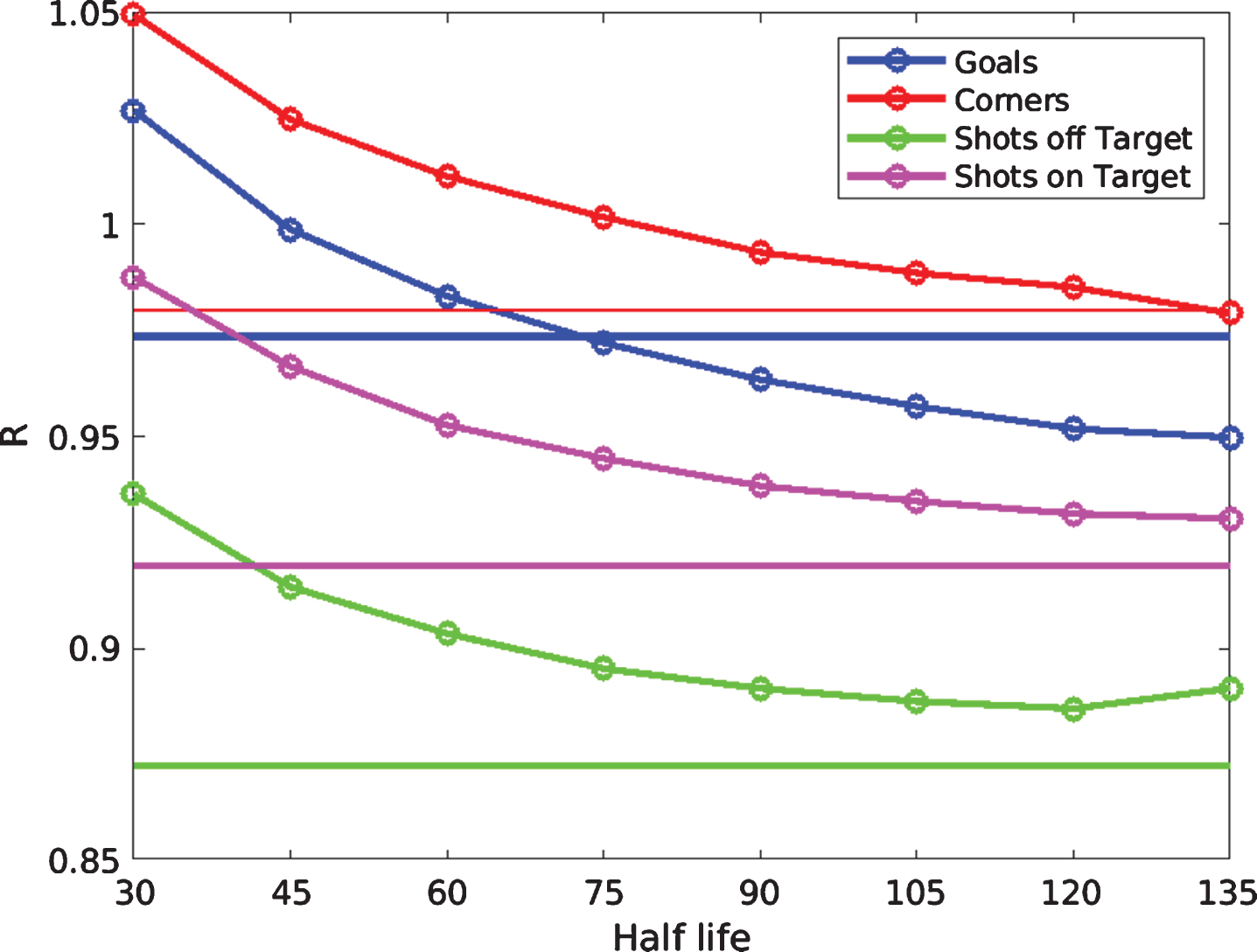
There is a notably high degree of variation in the performance of the predicted statistics. Under the GAP rating system, the value of R is smallest for shots off target, whilst for goals and corners, R is not much smaller than 1. This is likely explained by the fact that there are typically a larger number of shots off target in a game than the other statistics and therefore there is more information on which to base the forecasts. BA ratings do not outperform GAP ratings for match statistics other than goals for any tested half life.
5Variable selection
Our next focus is on variable selection and the aim is to find the combination of (i) observed and (ii) predicted match statistics that explain the match outcomes most effectively. Variable selection is performed using Akaike’s Information Criterion (AIC), which weighs up the fit of the model to the data with the number of parameters selected in-sample (see appendix A for details). As required for the calculation of information criteria, the ordinal regression parameters are selected in-sample and therefore, in order to calculate the likelihood, a single set of parameters is selected over all available matches.
To provide further context to the calculated AIC values, we make use of the confidence set approach described by Anderson and Burnham (2004). Here, the Akaike weights for each model (which can be thought of as the probability that each one represents the best approximating model) are calculated and sorted from largest to smallest. Models are then added to the confidence set in order of their Akaike weights (largest first) until the sum of the weights exceeds 0.95. The confidence set then represents the set in which the best approximating model falls with at least 95 percent probability.
5.1Variable selection: observed match statistics
The results of variable selection when using observed match statistics are shown in Table 2. Here, the AIC for different combinations of statistics is shown both with and without the home odds-implied probability included as an additional predictor variable. Note that the AIC in each case is expressed with that of model A0 (fitted without the odds-implied probability) subtracted such that negative values imply better support for a particular combination of predictor variables than that of the model fitted without any predictor variables. The lower the AIC, the more support for that particular combination of variables.
Table 2
AIC of each combination of observed match statistics with and without the home odds-implied probability included as a predictor variable. Variables that are included are denoted with a star and, in each case, AIC is given with that of model A0 subtracted. The combination of variables with the lowest AIC is highlighted in bold and each one that falls into the 95 percent confidence set is highlighted in green (which is only combination A1 in this case)
| Combination of variables | Shots on Target | Shots off Target | Corners | AIC w/o odds | AIC w. odds |
| A1 | * | * | * | - 15125.4 | - 19473.6 |
| A3 | * | * | -14804.3 | -18572.7 | |
| A2 | * | * | -13530.9 | -17124.8 | |
| A4 | * | -12239.9 | -14643.5 | ||
| A5 | * | * | -18.5 | -9150.4 | |
| A6 | * | -18.3 | -8658.7 | ||
| A7 | * | -9.2 | -8598.3 | ||
| A0 | 0 | -5619.1 |
The results yield a number of conclusions. The best AIC is achieved when the model includes all three observed match statistics both when the home odds-implied probability is included as an additional predictor variable and when it is not. That the number of shots on target should have an impact on the match result should not come as a surprise, since all goals other than own goals and highly unusual events (such as the ball deflecting off the referee or, in one case in 2009, a beachball) result from a shot on target. Interestingly, however, the inclusion of the number of corners and shots off target, which don’t usually directly result in goals, improves the model even once shots on target are considered.
It is also interesting to compare the effects of each observed match statistic as an individual predictor variable. Unsurprisingly, the number of shots on target provides the most information, followed by corners and shots off target. Interestingly, shots off target and corners do not provide much information when considered individually but add a great deal of information when combined with the number of shots on target and/or the home odds-implied probability. It is a property of generalised linear models that some predictor variables are only informative in combination with other predictor variables and this appears to be the case here.
Finally, all three match statistics add information even when the odds-implied probability is included in the model. This is perhaps not surprising since match statistics give an indication of how the match actually went.
In practice, of course, observed statistics are never available pre-match. Despite this, the results shown here have important implications. Match statistics can be predicted and, if those predictions are informative enough, it stands to reason that informative forecasts of the outcome of the match can be made.
5.2Variable selection: predicted match statistics
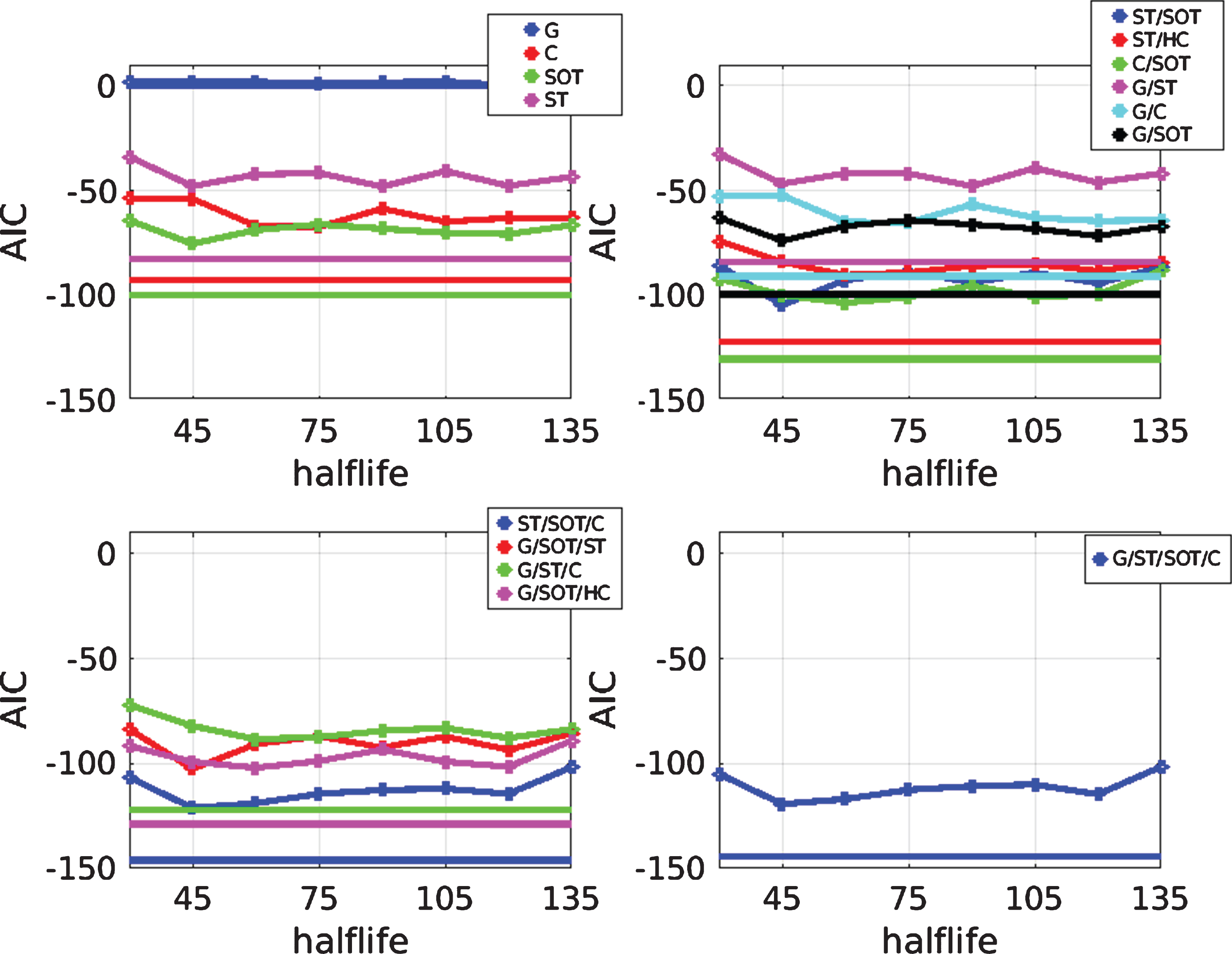
In section 4.2, the results of predicting match statistics using GAP and BA ratings were presented. It was shown that, in the latter case, the choice of half life has an important impact on the MAE of the predictions. Although, typically, longer half lives tend to provide better predictions for the match statistics, it may not be the case that they provide a more useful input for probabilistic forecasts of the match outcome. This is because a consistently strong team like, say, Manchester United will be expected to take a larger number of shots and corners than a weaker side over a long period of time and this will be reflected in the ratings. However, we are looking for information that is not reflected in the odds and thus to augment the information the odds provide. For example, if a team’s recent results have not reflected their performances, we look to identify that this is the case from their match statistics in recent matches. It therefore seems reasonable to expect that a shorter half life should be more useful in this case. On the other hand, looking only at more recent matches gives us a less robust reflection of a team’s strength and we therefore have a trade-off. Here, for simplicity, we choose a single half life for use in the rest of the paper based on the following fairly ad-hoc approach. Looking at the results in Fig. 2, since a half life of 45 days gives the lowest AIC for the case in which predictions of all match statistics are used in the model (bottom right panel), this value is used for all further results shown in this paper.
Fig. 2
AIC as a function of half life for forecasts produced using different combinations of (i) BA ratings (lines with points) and (ii) GAP ratings (straight horizontal lines). In both cases, the home odds-implied probability is used as an additional predictor variable.
The results of variable selection with predicted match statistics are shown in Table 3. Unsurprisingly, the AIC is generally higher than for the observed case, implying that the information content is lower. Despite this, predicted match statistics are able to provide information regarding match outcomes, even when the home odds-implied probability is included in the model. This means that, on average, both sets of predicted match statistics (from GAP and BA ratings) provide information beyond that contained in the odds-implied probabilities. However, given the universally lower AIC values, the GAP rating approach appears to be more effective.
Table 3
AIC of each combination of predicted match statistics under both GAP and BA ratings with and without the home odds-implied probability included as a predictor variable. Included variables are denoted with a star and each AIC value is given relative to that of the regression model with only a constant term. The combination of variables with the lowest AIC is highlighted in bold and each one that falls into the 95 percent confidence set is highlighted in green
| Combination of variables | Goals | Shots on Target | Shots off Target | Corners | GAP:AIC w/o odds | GAP:AIC w. odds | BA:AIC w/o odds | BA:AIC w. odds |
| B1 | * | * | * | -5453.6 | - 7619.9 | -4405.5 | - 7595.0 | |
| B9 | * | * | * | * | - 6365.0 | -7618.5 | - 5363.4 | -7593.2 |
| B2 | * | * | -5359.5 | -7604.3 | -4176.2 | -7578.5 | ||
| B5 | * | * | -4124.4 | -7604.1 | -2959.1 | -7573.7 | ||
| B10 | * | * | * | -6309.5 | -7602.9 | -5153.1 | -7576.5 | |
| B13 | * | * | * | -6268.3 | -7602.7 | -4914.3 | -7573.0 | |
| B11 | * | * | * | -6245.6 | -7596.1 | -5072.4 | -7555.9 | |
| B3 | * | * | -5357.5 | -7596.0 | -4072.2 | -7557.9 | ||
| B7 | * | -3286.5 | -7573.5 | -2185.0 | -7549.2 | |||
| B15 | * | * | -6146.9 | -7573.3 | -4481.4 | -7547.8 | ||
| B6 | * | -3499.6 | -7566.5 | -2063.6 | -7527.8 | |||
| B14 | * | * | -6051.3 | -7564.8 | -4405.6 | -7526.2 | ||
| B12 | * | * | -6087.3 | -7557.9 | -4631.3 | -7520.7 | ||
| B4 | * | -5146.7 | -7556.5 | -3583.2 | -7521.8 | |||
| B0 | 0.0 | -7473.9 | 0.0 | -7473.9 | ||||
| B8 | * | -5573.3 | -7473.9 | -3342.7 | -7471.9 |
It is of interest to note the relative importance of the different predicted match statistics. Consistent with the findings of Wheatcroft (2020), the predicted number of goals provides relatively little information when combined with the odds-implied probabilities whilst predictions of other match statistics are much more effective in improving the forecast model. It is also notable that whilst, in the observed case, the number of shots on target provides the most information about the outcome of the match, in the predicted case, shots off target is the most informative. At first, this seems counterintuitive. However, it should be noted that the information in the prediction is dependent both on the impact of the observed statistic on the match and the quality of the prediction of that statistic. Recall that Fig. 1 suggests GAP and BA rating predictions of shots off target improve more on the mean-benchmark model than those of the other match statistics and this superior prediction accuracy is the likely explanation.
Finally, it is notable that, when considered as individual predictor variables, the predicted number of shots off target and corners outperforms the equivalent observed statistics. Again, this seems counterintuitive but can probably be explained by the fact that the predicted values consider the performances of the teams over multiple past matches, gaining some information about the relative strengths of the two teams.
5.3Forecast performance
We now turn our focus onto the question of forecast performance. Though closely related to model selection, this allows us to assess the relative performance of the forecasts out-of sample and therefore as if they were produced in real time. In order to produce the forecasts, new regression parameters are selected on each day in which at least one match is played and are calculated based on all past matches which fall outside of the ‘burn-in’ period and which have shots and corner data as well as match odds available.
We compare forecast performance using two commonly used scoring rules: the Ignorance Score (Roulston and Smith, 2002; Good, 1952) and the Ranked Probability Score (Constantinou and Fenton, 2012). The ignorance score, also commonly known as the log-loss is given by
(19)
To define the Ranked Probability Score, for an event with r possible outcomes, let pj and oj be the forecast probability and outcome at position j where the ordering of the positions is preserved. The Ranked Probability Score (RPS) is given by
(20)
The RPS is often considered appropriate for evaluating forecasts of football matches because it takes into account the ordering of the outcomes, i.e. a home win is ‘closer’ to a draw than it is to an away win (Constantinou and Fenton, 2012). However, it has also been argued that the ordered nature of the RPS provides little practical benefit and that only the probability placed on the outcome should be taken into account, as per the ignorance score (Wheatcroft, 2019). Here, we consider it useful to evaluate the forecasts using both approaches.
To provide some context regarding the performance of the forecasts, we compare the performance with that of an alternative, strongly performing approach to forecasting football matches. The Bivariate Poisson model, described in Section 2.3, has been shown to perform favourably with respect to 9 other forecast models (Ley et al., 2019). We apply the model to our data set using the optimal half life parameter of 390 days determined by Ley et al. (2019).
Similarly to the Akaike weights confidence set used in section 5, we take a similar approach here using the Model Confidence Set (MCS) methodology proposed by Hansen et al. (2011). Here, the aim is to identify the set of models in which there is a 95 percent probability that the ‘best’ model falls, given the chosen measure of performance. We highlight the combinations of variables that fall into this set.
The mean RPS and Ignorance of each combination of variables as well as the Bivariate Poisson model are shown in Tables 4 and 5, respectively. In the latter case, the scores are given with that of model B0 subtracted such that negative scores imply better performance than the model applied with no predictor variables. The 95 percent Model Confidence Set in each case is highlighted in green. Note that, since the Bivariate Poisson model does not make use of match odds, a fair comparison is only provided by comparing these combination of variables in which the odds-implied probabilities are not included.
Table 4
Mean RPS for each combination of variables and, for comparison, that of the Bivariate Poisson model. Included variables are denoted with a star. The combination with the highest performance is highlighted in bold and each one that falls into the Model Combination Set is highlighted in green
| Combination of variables | Goals | Shots on Target | Shots off Target | Corners | GAP:RPS w/o odds | GAP:RPS w. odds | BA:RPS w/o odds | BA:RPS w. odds |
| B5 | * | * | 0.2149 | 0.2058 | 0.2191 | 0.2059 | ||
| B9 | * | * | * | * | 0.2090 | 0.2058 | 0.2128 | 0.2059 |
| B2 | * | * | 0.2116 | 0.2058 | 0.2161 | 0.2059 | ||
| B1 | * | * | * | 0.2113 | 0.2058 | 0.2154 | 0.2059 | |
| B13 | * | * | * | 0.2093 | 0.2058 | 0.2140 | 0.2059 | |
| B10 | * | * | * | 0.2092 | 0.2058 | 0.2135 | 0.2059 | |
| B11 | * | * | * | 0.2093 | 0.2058 | 0.2136 | 0.2060 | |
| B7 | * | 0.2171 | 0.2059 | 0.2212 | 0.2060 | |||
| B3 | * | * | 0.2116 | 0.2058 | 0.2163 | 0.2060 | ||
| B6 | * | 0.2166 | 0.2059 | 0.2214 | 0.2060 | |||
| B14 | * | * | 0.2099 | 0.2059 | 0.2153 | 0.2060 | ||
| B15 | * | * | 0.2096 | 0.2059 | 0.2152 | 0.2060 | ||
| B12 | * | * | 0.2098 | 0.2059 | 0.2150 | 0.2061 | ||
| B4 | * | 0.2121 | 0.2059 | 0.2178 | 0.2061 | |||
| B0 | 0.2264 | 0.2062 | 0.2264 | 0.2062 | ||||
| B8 | * | 0.2111 | 0.2062 | 0.2182 | 0.2062 | |||
| Bivariate Poisson | * | 0.2121 | 0.2121 |
Table 5
Mean ignorance scores for each combination of variables and, for comparison, that of the Bivariate Poisson model. Included variables are denoted with a star. The combination with the highest performance is highlighted in bold and each one that falls into the Model Combination Set is highlighted in green
| Combination of variables | Goals | Shots on Target | Shots off Target | Corners | GAP:IGN w/o odds | GAP:IGN w. odds | BA:IGN w/o odds | BA:IGN w. odds |
| B9 | * | * | * | * | - 0.0739 | - 0.0888 | - 0.0626 | - 0.0887 |
| B1 | * | * | * | -0.0635 | -0.0888 | -0.0516 | -0.0887 | |
| B2 | * | * | -0.0624 | -0.0887 | -0.0490 | -0.0886 | ||
| B10 | * | * | * | -0.0733 | -0.0886 | -0.0602 | -0.0886 | |
| B5 | * | * | -0.0480 | -0.0887 | -0.0345 | -0.0885 | ||
| B13 | * | * | * | -0.0728 | -0.0886 | -0.0572 | -0.0885 | |
| B11 | * | * | * | -0.0727 | -0.0887 | -0.0592 | -0.0883 | |
| B7 | * | -0.0382 | -0.0883 | -0.0257 | -0.0883 | |||
| B3 | * | * | -0.0625 | -0.0887 | -0.0477 | -0.0883 | ||
| B15 | * | * | -0.0714 | -0.0883 | -0.0522 | -0.0882 | ||
| B6 | * | -0.0410 | -0.0884 | -0.0241 | -0.0880 | |||
| B14 | * | * | -0.0704 | -0.0884 | -0.0513 | -0.0880 | ||
| B12 | * | * | -0.0709 | -0.0883 | -0.0541 | -0.0880 | ||
| B4 | * | -0.0601 | -0.0883 | -0.0421 | -0.0880 | |||
| B0 | 0.0000 | -0.0875 | 0.0000 | -0.0875 | ||||
| B8 | * | -0.0650 | -0.0874 | -0.0388 | -0.0875 | |||
| Bivariate Poisson | * | -0.0614 | -0.0614 |
Similarly to the variable selection results in section 5.3, including predictions of match statistics other than goals in the model improves overall predictive performance of the match outcomes according to both scoring rules. Also consistent with the model selection results is that the model performs consistently better when match statistics are predicted using GAP ratings rather than BA ratings.
When considering the performance of the Bivariate Poisson model, it is worth noting that it only takes goals into consideration. In terms of the information used, its performance can be compared with model B8 for the case in which the odds-implied probability is not included. Here, the Bivariate Poisson model does slightly worse though the difference is small. It is when predictions of other match statistics are included that there is a large increase in performance over the Bivariate Poisson model. This suggests that much of the improvement results from the additional information in the match statistics rather than the structure of the model.
5.4Betting performance
In this section, the performance of the forecasts in section 5.3 when used alongside the Level Stakes and Kelly betting strategies described in section 3.3 is assessed. Here, it is assumed that a gambler is able to ‘shop around’ different bookmakers and take advantage of the highest odds offered on each outcome. The maximum odds over all available bookmakers are thus assumed to be obtainable (note that the actual bookmakers included in the data set vary over time). Note that bets placed on draws are not considered due to the inherent difficulty of predicting them and therefore only bets on home or away wins are allowed. The mean percentage profit obtained from the Level Stakes betting strategy when used alongside forecasts derived from each combination of predicted match statistics is shown in Table 6, along with 95 percent bootstrap resampling intervals. The resampling intervals are presented to demonstrate the robustness of the profit and, if the interval does not contain zero, the profit can be considered to be statistically significant.
Table 6
Mean percentage profit of Level Stakes strategy with each combination of predicted match statistics with and without odds-implied probabilities included as a predictor variable. Included variables are denoted with a star
| Combination of variables | Goals | Shots on Target | Shots off Target | Corners | GAP:Profit w/o odds | GAP:Profit w. odds | BA:Profit w/o odds | BA:Profit w. odds |
| B5 | * | * | +0.54 (-0.83, + 1.98) | + 1.85 (+0.45, + 3.34) | -0.29 (-1.68, + 1.15) | + 1.41 (-0.10, + 3.09) | ||
| B9 | * | * | * | * | +0.60 (-0.89, + 2.09) | +1.55 (+0.32, + 3.12) | +0.23 (-1.37, + 1.73) | +1.24 (+0.01, + 2.59) |
| B2 | * | * | +0.36 (-1.00, + 1.76) | +1.73 (+0.23, + 3.18) | +0.07 (-1.51, + 1.32) | +1.28 (-0.30, + 2.85) | ||
| B1 | * | * | * | + 0.67 (-1.07, + 1.88) | +1.48 (-0.11, + 2.79) | + 0.25 (-1.02, + 1.68) | +1.30 (-0.11, + 2.80) | |
| B13 | * | * | * | +0.33 (-1.23, + 2.07) | +1.77 (+0.20, + 3.01) | -0.18 (-1.67, + 1.41) | +1.26 (-0.16, + 2.78) | |
| B10 | * | * | * | +0.02 (-1.42, + 1.71) | +1.60 (+0.07, + 3.12) | -0.63 (-2.18, + 0.78) | +1.21 (+0.05, + 2.83) | |
| B11 | * | * | * | +0.00 (-1.31, + 1.58) | +0.93 (-0.80, + 2.32) | -0.43 (-1.88, + 0.89) | +0.76 (-0.54, + 2.53) | |
| B7 | * | -0.44 (-2.05, + 0.79) | +1.15 (-0.52, + 2.78) | -0.89 (-2.17, + 0.67) | +0.85 (-0.51, + 2.38) | |||
| B3 | * | * | +0.37 (-1.20, + 1.88) | +1.00 (-0.28, + 2.49) | -0.23 (-1.45, + 1.22) | +0.81 (-0.60, + 2.42) | ||
| B6 | * | -0.74 (-2.26, + 0.69) | +1.16 (-0.23, + 2.67) | -1.15 (-2.66, + 0.27) | +0.43 (-1.17, + 2.04) | |||
| B14 | * | * | -0.62 (-2.00, + 0.82) | +0.83 (-0.40, + 2.15) | -1.02 (-2.53, + 0.49) | +0.33 (-1.49, + 1.60) | ||
| B15 | * | * | -0.41 (-1.67, + 1.09) | +0.83 (-0.40, + 2.15) | -1.03 (-2.39, + 0.33) | +0.84 (-0.45, + 2.42) | ||
| B12 | * | * | -1.07 (-2.63, + 0.26) | +0.46 (-0.88, + 2.01) | -1.08 (-2.77, + 0.25) | -0.34 (-1.49, + 1.81) | ||
| B4 | * | -0.44 (-1.89, + 1.04) | +0.13 (-1.42, + 1.89) | -0.74 (-2.25, + 0.95) | -0.36 (-1.66, + 1.36) | |||
| B0 | -2.33 (-3.84, - 0.73) | -1.26 (-3.06, + 0.48) | -2.33 (-3.55, - 1.02) | -1.26 (-3.20, + 0.20) | ||||
| B8 | * | -2.69 (-4.22, - 1.32) | -1.70 (-3.41, - 0.34) | -2.84 (-4.28, - 1.55) | -1.37 (-2.94, + 0.48) |
It is clear from the results that including combinations of predicted match statistics as predictor variables tends to yield a profit. In addition, for all combinations, including the home odds-implied probability as an additional predictor variable yields an increase in profit. In some cases, when the home odds-implied probability is included, the profit is significant, i.e. the bootstrap resampling interval does not include zero. Whilst caution is advised in comparing the precise rankings of different combinations of variables, the best performing combinations tend to include the predicted number of shots off target. The predicted number of goals, on the other hand, tends to have limited value. When individual predicted statistics are considered, the ranking of the results is consistent with the variable selection results of Table 3 in that the best performing predicted variable is shots off target, followed by corners, shots on target and goals. It is also notable that forecasts built using BA ratings do not perform as well as those formed using GAP ratings.
The mean profit obtained from using the forecasts alongside the Kelly strategy are shown in Table 7. Here, under both the GAP and BA rating systems, notably, the mean profit is generally substantially higher than that achieved using the Level Stakes strategy. Again, including the home odds-implied probability as an additional predictor variable yields improved results for all combinations of variables. In fact, the profit is significant in all cases in which at least one predicted match statistic other than the number of goals is included alongside the home odds-implied probability. Again, the results obtained from the GAP rating approach are almost always better than under the BA rating approach.
For the remainder of this section, given the superior performance of GAP ratings relative to the BA ratings, we focus on the betting performance of forecasts formed using predicted shots on target, shots off target and corners simultaneously under this approach. We do this both with and without the home odds-implied probability as an additional predictor variable.
Table 7
Mean percentage profit from the Kelly strategy using forecasts based on each combination of predicted match statistics with and without the home odds-implied probability included as a predictor variable. Included variables are denoted with a star
| Combination of variables | Goals | Shots on Target | Shots off Target | Corners | GAP:Profit w/o odds | GAP:Profit w. odds | BA:Profit w/o odds | BA:Profit w. odds |
| B1 | * | * | * | + 3.72 (+1.61, + 5.48) | + 4.88 (+3.22, + 6.39) | + 3.13 (+1.27, + 5.01) | + 4.27 (+2.61, + 5.85) | |
| B9 | * | * | * | * | +2.33 (+0.20, + 4.15) | +4.87 (+3.41, + 6.45) | +2.46 (+0.58, + 4.27) | +4.24 (+2.73, + 5.84) |
| B10 | * | * | * | +2.14 (+0.45, + 3.93) | +4.66 (+3.05, + 6.21) | +1.87 (+0.04, + 3.68) | +3.90 (+2.12, + 5.45) | |
| B2 | * | * | +3.45 (+1.51, + 5.33) | +4.67 (+3.11, + 6.11) | +2.48 (+0.60, + 4.60) | +3.94 (+2.26, + 5.58) | ||
| B5 | * | * | +2.93 (+1.04, + 5.06) | +4.56 (+3.06, + 6.12) | +2.10 (+0.03, + 4.20) | +3.93 (+2.37, + 5.65) | ||
| B13 | * | * | * | +1.79 (-0.01, + 3.67) | +4.52 (+2.97, + 6.14) | +1.71 (-0.20, + 3.54) | +3.89 (+2.22, + 5.53) | |
| B11 | * | * | * | +1.36 (-0.57, + 3.38) | +4.02 (+2.39, + 5.67) | +0.90 (-0.98, + 2.78) | +2.55 (+1.00, + 4.18) | |
| B7 | * | +2.02 (+0.27, + 4.01) | +4.09 (+2.44, + 5.66) | +0.66 (-1.56, + 2.76) | +3.25 (+1.64, + 4.99) | |||
| B3 | * | * | +2.97 (+1.09, + 4.90) | +4.00 (+2.25, + 5.67) | +1.71 (-0.27, + 3.82) | +2.58 (+0.93, + 4.22) | ||
| B15 | * | * | +1.26 (-0.60, + 3.13) | +4.07 (+2.45, + 5.75) | +0.54 (-1.36, + 2.31) | +3.23 (+1.62, + 4.84) | ||
| B12 | * | * | +0.52 (-1.42, + 2.60) | +2.92 (+1.19, + 4.64) | -0.22 (-2.15, + 1.73) | +1.35 (-0.47, + 3.15) | ||
| B6 | * | +1.18 (-0.84, + 3.31) | +2.96 (+1.38, + 4.62) | +0.16 (-1.89, + 2.25) | +1.78 (-0.12, + 3.53) | |||
| B14 | * | * | +0.05 (-1.87, + 2.01) | +2.97 (+1.31, + 4.62) | -0.36 (-2.19, + 1.55) | +1.74 (+0.07, + 3.41) | ||
| B4 | * | +2.14 (+0.29, + 4.16) | +2.85 (+1.30, + 4.44) | +0.58 (-1.48, + 2.63) | +1.33 (-0.45, + 3.13) | |||
| B8 | * | -2.64 (-4.77, - 0.75) | -1.36 (-3.31, + 0.73) | -3.07 (-5.29, - 0.80) | -1.11 (-3.17, + 0.91) | |||
| B0 | -3.07 (-5.51, - 0.66) | -1.06 (-3.17, + 0.99) | -3.12 (-5.60, - 0.59) | -1.06 (-3.27, + 1.04) |
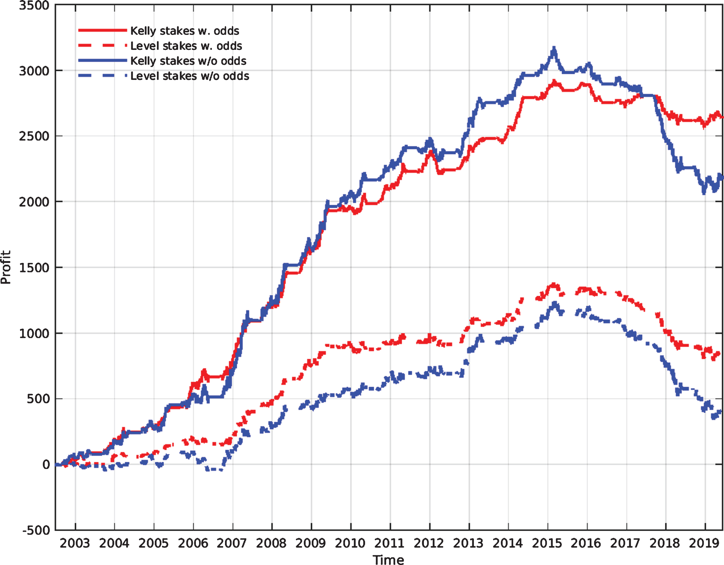
The cumulative profit achieved with each of the two betting strategies is shown in Fig. 3. As already shown in Tables 6 and 7, a substantial profit is made in all four cases. The figure, however, shows how each strategy performs over time and an interesting feature is that there appears to be a downturn in profit in recent seasons. Whilst this could conceivably be explained by random chance, it is perhaps more likely that something fundamental changed over that time. That predicted match statistics provide information additional to that contained in the odds suggests that, in general, the odds do not adequately account for the ability of teams to create shots and corners. However, as more data have become available and quantitative analysis has become more sophisticated, it seems a reasonable claim that such information is now more likely to be reflected in the odds on offer and it may therefore be the case that the betting opportunities available in earlier seasons simply don’t exist anymore.
Fig. 3
Cumulative profit from using the Kelly strategy (solid lines) and the level stakes strategy (dashed lines) with forecasts formed using GAP rating predictions of shots on target, shots off target and corners both when the home odd-implied probability is included as a predictor variable in the model (blue) and when it is excluded (red).
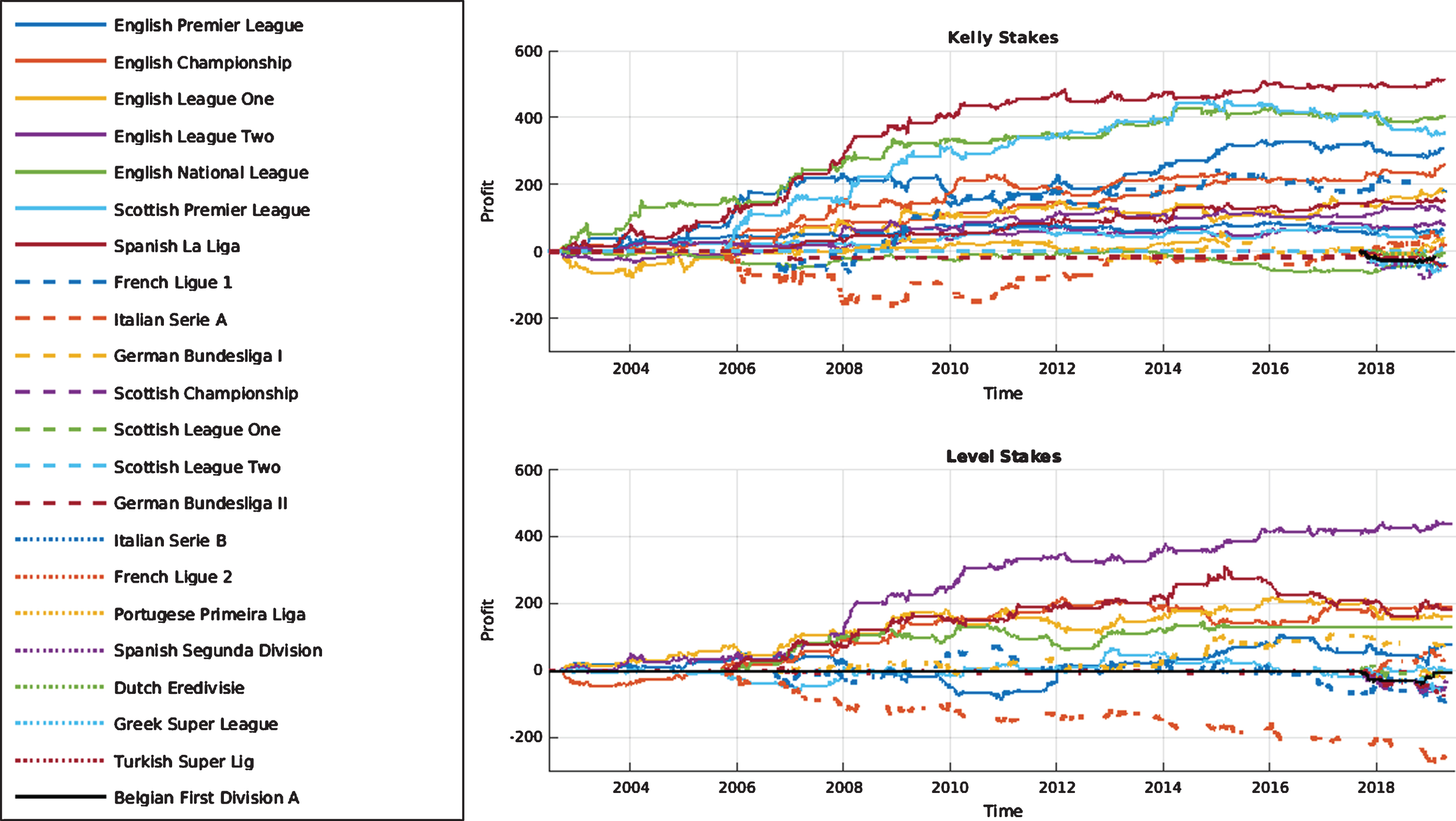
It is worth considering how the profits from each betting strategy are distributed between the different leagues and whether losses in any particular subset of leagues can explain the observed downturn. Focusing on the case in which the home odds-implied probability is included as a predictor variable, in Fig. 4 the cumulative profit made in each league is shown as a function of time. Here, the decline in profit appears to be fairly consistent over all leagues considered and therefore, if the information reflected in the odds really has increased over time, this appears to be fairly universal over the different leagues.
Fig. 4
Cumulative profit as a function of time in each league for the case in which predicted shots on target, shots off target and corners along with the home odds-implied probability are included as predictor variables.
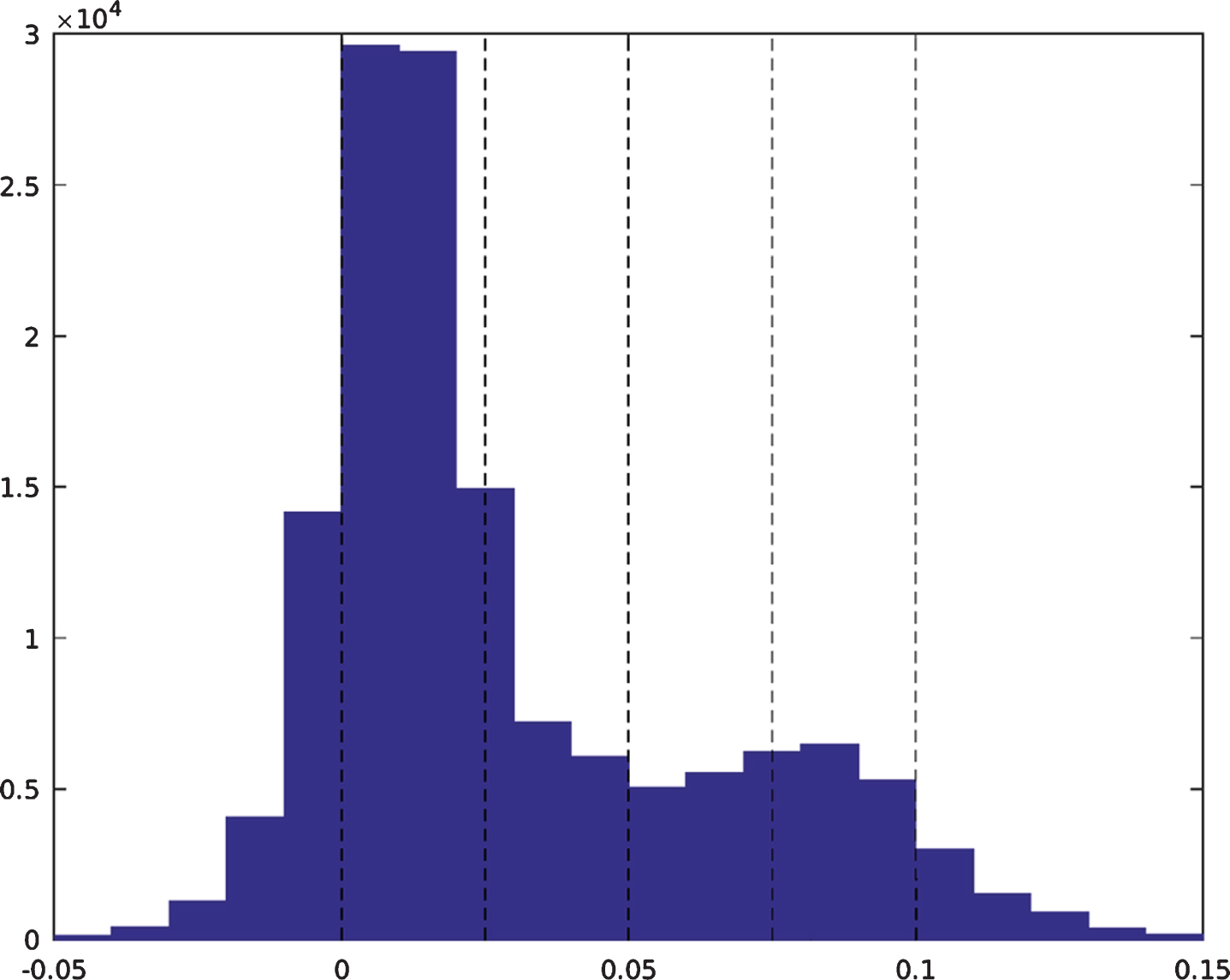
Finally, it is important to assess the impact of the overround on the profitability of the betting strategies. In this experiment, it is assumed that the gambler is able to find the best odds on offer on each possible outcome, over a range of bookmakers. Due to increased competition, there has been a trend towards reduced profit margins in recent years. This can have a knock on effect on the overround of the best odds. A histogram of the overround of the best odds for all matches deemed eligible for betting is shown in Fig. 5. Whilst, in the majority of cases, the overround is positive, in around 18 percent of cases, it is negative. This gives rise to arbitrage opportunities, which means that a guaranteed profit can be made, without any need for a model. It is therefore important to distinguish cases in which profits are made due to the performance of the forecasts from those in which a profit could be guaranteed through arbitrage.
Fig. 5
Histogram of overrounds under the maximum odds.
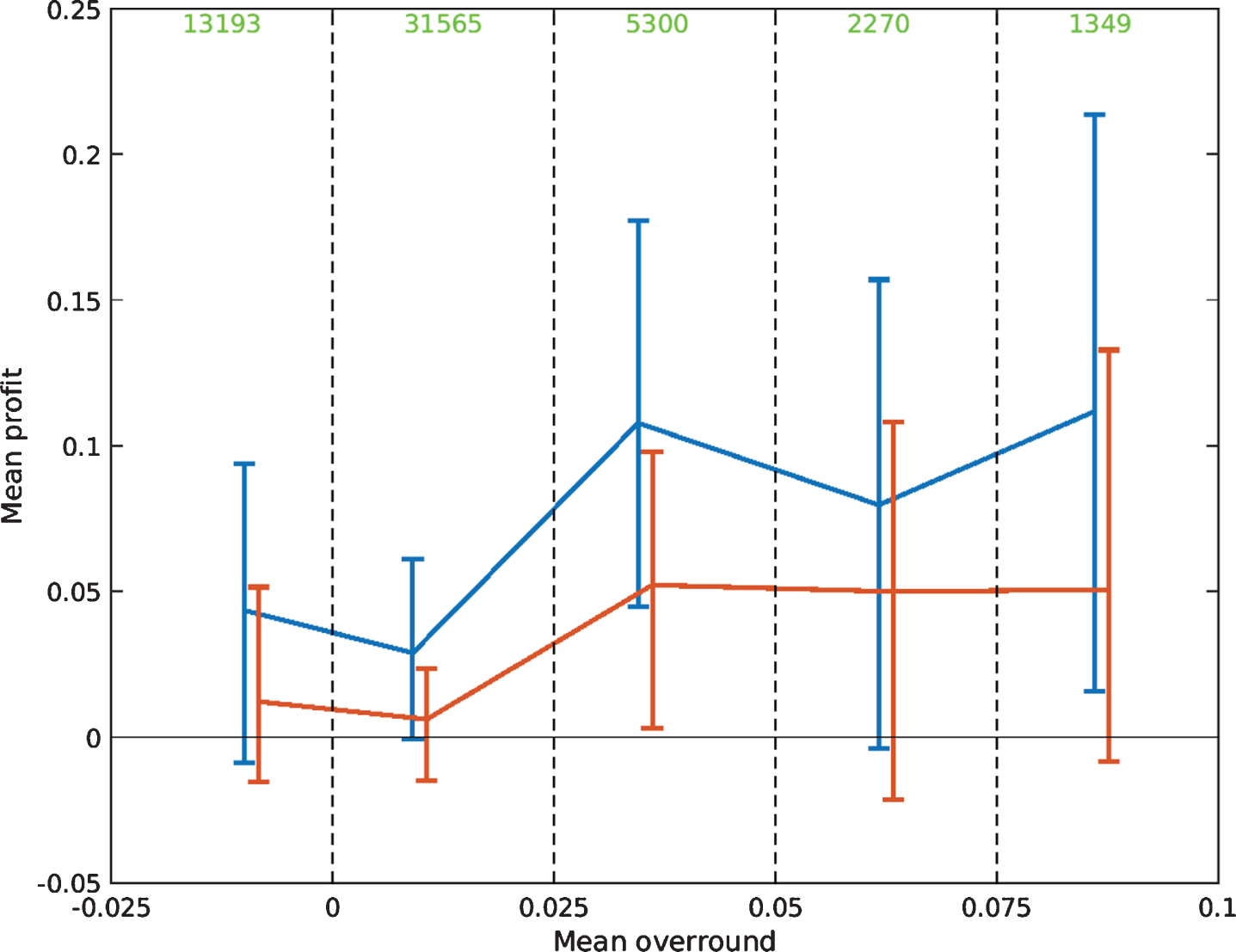
To assess the importance of the overround, five different intervals are defined and the mean profit from matches whose overround falls into each one is calculated under both betting strategies. The first interval contains all matches with an overround less than zero, whilst, for matches with a positive overround, intervals with a width of 2.5 percent are defined. The interval containing matches with the largest overrounds consider those in which the overround is greater than 7.5 percent. In Fig. 6, the mean overround for matches contained in each interval is plotted against the mean profit under each of the two betting strategies. The error bars correspond to 95 percent bootstrap resampling intervals of the mean profit. In all five intervals, and under both betting strategies, the mean profit is positive. Under the Kelly strategy, three out of the five intervals yield a significant profit, whilst this is true in one interval for the Level Stakes strategy. Interestingly, the mean profit is not significantly different from zero when the overround is negative. This, however, is consistent with the decline in profit in recent seasons that has tended to coincide with lower overrounds. Overall, the fact that significant profits can be made for matches in which the overround is positive suggest that, over the course of the dataset, the forecasts in combination with the two betting strategies would have been successful in identifying profitable betting opportunities.
Fig. 6
Mean overround against mean profit under the Kelly strategy (blue) and the Level Stakes strategy (red) for each considered interval. The error bars represent 95 percent bootstrap resampling intervals of the mean.
6Discussion
In this paper, relationships between observed and predicted match statistics and the outcomes of football matches have been assessed. Unsurprisingly, the observed number of shots on target is a strong predictor of the match outcome whilst the observed numbers of shots off target and corners also provides some predictive value, once the number of shots on target and/or the match odds are taken into account. With this in mind, the key claim of this paper is that predictions of match statistics, if accurate enough, can be informative about the outcome of the match and, crucially, since the predictions are made in advance, this can aid betting decisions.
Both GAP and BA ratings have been demonstrated to provide a convenient and straightforward approach to the prediction of match statistics. The former, however, has been shown to perform consistently better in terms of predicting match outcomes. A number of other interesting, and perhaps surprising, conclusions have been revealed. Notably, in the prediction of match results, the most informative observed statistics do not coincide with the most informative predicted statistics. Whilst the number of shots on target was found to be the most informative observed statistic, the most informative predicted statistic was found to be the number of shots off target. As pointed out earlier in the paper, this can likely be explained by the fact that the information in the predicted statistics reflects both the importance of the statistic itself, in terms of the match outcome, and the accuracy of the prediction of that statistic. That there is agreement on this between GAP and BA ratings provides further evidence for this claim.
The observation above has interesting implications for the philosophy of sports prediction. The importance of match statistics and, in particular, statistics such as expected goals that are derived from match events is becoming clear. The aim of expected goals can broadly be considered to be to estimate the expected number of goals a team ‘should’ score, given the location and nature of the shots it has taken. A shot taken close to the goal and at a favourable angle has a high chance of being successful and therefore contributes more to a team’s expected goals than a shot that is far away and from which it is difficult to score. As such, expected goals ought to reflect the likelihood of each match outcome better than traditional statistics like the number of shots on target. The results in this paper, however, suggest that it is not necessarily the case that predictions of the number of expected goals by each team would outperform predictions of, or ratings based on, other statistics. Interesting future work would therefore be to predict the number of expected goals in a similar way to that demonstrated in this paper to assess the effect on the forecasting of match outcomes.
The results in this paper inspire a number of future avenues for research. There is a wide and growing range of betting markets available for football matches and GAP ratings may be useful in informing such bets. This has already been shown by Wheatcroft (2020) in the over/under 2.5 goal market but could also be applied to other markets such as Asian Handicap, the number of shots taken in a match, half time results and many more. The philosophy demonstrated in this paper could also be applied to other sports. For example, in ice hockey, GAP ratings could be used to estimate the number of shots at goal, whilst, in American Football, they could be used to predict the number of yards gained by each team in the match.
Another interesting feature of the results presented in this paper is the decline in profit over the last few seasons. This was briefly discussed in the results section and it was suggested that betting odds may now incorporate more information than at the beginning of the data set. It would be interesting to investigate this further.
This paper demonstrates a new way of thinking about match statistics and their relationship with the outcomes of football matches and sporting events in general. It is hoped that this can help provide a better understanding of the role of match statistics in sports prediction and GAP ratings provide a straightforward and intuitive way in which to do this.
References
[1] | Anderson, D and Burnham, K. (2004) , Model selection and multi-model inference, Second. NY: Springer-Verlag, 63: (2020), 10. |
[2] | Baker, R. D and McHale, I. G. (2015) , Time varying ratings in association football: the all-time greatest team is, Journal of the Royal Statistical Society: Series A (Statistics in Society) 178: (2), 481–492. |
[3] | Boshnakov, G , Kharrat, T and McHale, I. G. (2017) , A bivariate Weibull count model for forecasting association football scores, International Journal of Forecasting 33: (2), 458–466. |
[4] | Carbone, J , Corke, T and Moisiadis, F. (2016) , The Rugby League Prediction Model: Using an Elo-based approach to predict the outcome of National Rugby League (NRL) matches, International Educational Scientific Research Journal 2: (5), 26–30. |
[5] | Constantinou, A. C and Fenton, N. E. (2012) , Solving the problem of in-adequate scoring rules for assessing probabilistic football forecast models, Journal of Quantitative Analysis in Sports 8: (1). |
[6] | Constantinou, A. C and Fenton, N. E. (2013) , Determining the level of ability of football teams by dynamic ratings based on the relative discrepancies in scores between adversaries, Journal of Quantitative Analysis in Sports 9: (1), 37–50. |
[7] | Constantinou, A and Fenton, N. (2017) , Towards smart-data: Improving predictive accuracy in long-term football team performance, Knowledge-Based Systems 124: , 93–104. |
[8] | Dixon, M. J. & Coles, S. G. (2004) , Modelling association football scores and inefficiencies in the football betting market, Journal of the Royal Statistical Society: Series C (Applied Statistics) 46: (2), 265–280. |
[9] | Dixon, M. J and Pope, P. F. (2004) , The value of statistical forecasts in the UK association football betting market, International Journal of Forecasting 20: (4), 697–711. |
[10] | Eggels, H. (2016) , Expected goals in soccer: Explaining match results using predictive analytics, in The Machine Learning and Data Mining for Sports Analytics workshop, pp. 16. |
[11] | Elo, A. E. (1978) , The rating of chessplayers, past and present, Arco Pub. |
[12] | Fifa 2018, Revision of the FIFA / Coca-Cola World Ranking, https://resources.fifa.com/image/upload/fifa-world-ranking-technical-explanation-revision.pdf?cloudid=edbm045h0udbwkqew35a. Accessed: 27/04/2019. |
[13] | FiveThirtyEight 2020a, The complete history of the NFL, https://projects.fivethirtyeight.com/complete-history-of-the-nfl/. Accessed: 16/01/2020. |
[14] | FiveThirtyEight 2020b, NBA Elo Ratings, https://fivethirtyeight.com/tag/nba-elo-ratings/. Accessed: 16/01/2020. |
[15] | Goddard, J. (2005) , Regression models for forecasting goals and match results in Association Football, International Journal of Forecasting 21: (2), 331–340. |
[16] | Good, I. J. , Rational Decisions, Journal of the Royal Statistical Society. Series B (Methodological) 14: (1), 107–114. |
[17] | Hansen, P. R , Lunde, A and Nason, J. M. (2011) , The model confidence set, Econometrica 79: (2), 453–497. |
[18] | Hvattum, L. M and Arntzen, H. (2010) , Using ELO ratings for match result prediction in association football, International Journal of Forecasting 26: (3), 460–470. |
[19] | Karlis, D and Ntzoufras, I. (2003) , Analysis of sports data by using bivariate Poisson models, Journal of the Royal Statistical Society: Series D (The Statistician) 52: (3), 381–393. |
[20] | Karlis, D and Ntzoufras, I. (2009) , Bayesian modelling of football outcomes: using the Skellams distribution for the goal difference, IMA Journal of Management Mathematics 20: (2), 133–145. |
[21] | Kelly Jr, J. (1956) , A new interpretation of the information rate, Bell System Technical Journal 35: , 917–926. |
[22] | Koopman, S. J and Lit, R. (2015) , A dynamic bivariate Poisson model for analysing and forecasting match results in the English Premier League, Journal of the Royal Statistical Society. Series A (Statistics in Society) pp. 167-186. |
[23] | Lasek, J , Szlávik, Z and Bhulai, S. (2013) , The predictive power of ranking systems in association football, International Journal of Applied Pattern Recognition 1: (1), 27–46. |
[24] | Lee, A. J. (1997) , Modeling scores in the premier league: is Manchester United really the best? Chance 10: (1), 15–19. |
[25] | Ley, C , Van de Wiele, T and Van Eetvelde, H. (2019) , Ranking soccer teams on the basis of their current strength: A comparison of maximum likelihood approaches, Statistical Modelling 19: (1), 55–73. |
[26] | Maher, M. J. (1982) , Modelling association football scores, Statistica Neer-landica 36: (3), 109–118. |
[27] | Rathke, A. (2017) , An examination of expected goals and shot efficiency in soccer. |
[28] | Roulston, M. S and Smith, L. A. (2002) , Evaluating probabilistic forecasts using Information Theory, Monthly Weather Review 130: (6), 1653–1660. |
[29] | Rue, H and Salvesen, O. (2000) , Prediction and retrospective analysis of soccer matches in a league, Journal of the Royal Statistical Society: Series D (The Statistician) 49: (3), 399–418. |
[30] | Sullivan, C and Cronin, C. (2016) , Improving Elo rankings for sports experimenting on the English Premier League, Virginia Tech CSx824/ECEx424technical report. |
[31] | Suznjevic, M , Matijasevic, M and Konfic, J. (2015) , Application context based algorithm for player skill evaluation in MOBA games, in 2015 International Workshop on Network and Systems Support for Games (NetGames), IEEE, pp. 1-6. |
[32] | Wheatcroft, E. (2019) , Evaluating probabilistic forecasts of foot-ball matches: The case against the Ranked Probability Score, arXiv preprint arXiv:1908.08980. |
[33] | Wheatcroft, E. (2020) , A profitable model for predicting the over/under market in football, International Journal of Forecasting. |
Appendices
A Akaike’s Information Criterion (AIC)
Akaike’s Information Criterion (AIC) weighs up the likelihood of a model with the number of estimated parameters to provide an indication of the fit of the model out-of-sample. In the context of predicting football match outcomes, AIC is given by
(21)
where k is the number of estimated parameters and


