
Modeling and simulating durations of men’s professional tennis matches by resampling match features
Abstract
In this paper we analyze the factors impacting on the length of a men’s professional tennis match and propose a model to simulate matches’ durations. Two distinctive features of the model are that i) it considers all kinds of events that impact on the duration of a match and ii) it is based only on publicly available data. Once built, the model allows to analyze the impact of different formats or rule changes on matches’ duration. The model is built and validated using a dataset including 19,961 matches played in the period January 2011 – December 2018. The simulated and observed distributions of the durations are compared with an in-depth goodness-of-fit analysis. This points out that the model provides a good description of the real distribution both in the central part and in the tails. We also show that our model improves similar models present in the literature. Finally, several case studies are analyzed: the effect of abolishing the first service or the advantages or both; the new tie-break format at Wimbledon; and the introduction of fifth set tie-break at Roland Garros.
1Introduction
In recent years tennis’ governing boards have begun to consider introducing new rules or modifying the current matches’ format in order to reduce the length of tennis matches and to make the “product” tennis more attractive.
Reducing the length of matches is important because very long matches can make it difficult for tournaments to complete the schedule on time, mostly when there are also delays due to weather conditions. They also increase the risk of injury and physical stress for the players and, thus, of “retired matches”. From the audience point of view, there is concern that people may lose interest in tennis if very long matches become the norm. Finally, long matches are often difficult to manage by TV broadcasts.
Which is the best way to reach the goal, however, is still under discussion. To reduce injuries and increase fairness of matches, Pollard and Noble (2003) and Pollard and Noble (2004a) propose the use, also in single matches, of the no-advantage game, i.e. when the score is at deuce (40-40), players need only one point to win the game. They also propose the so-called “50-40 game”, i.e. the server is required to reach 50 (one point more than 40) while the receiver needs to reach only 40. Thus, the server has the advantage of serving but the disadvantage of having to win one more point than the receiver in order to win the game. The 50-40 game was also suggested by Barnett et al. (2006) to reduce the likelihood of long matches.
Pollard and Barnett (2018) explored some possible structures for “short games”. Besides the no-ad and the 50-40 game, they proposed i) the 30-30 advantage game, where the winner is the first player to win at least 3 points with at least 2 points more than the opponent; ii) the 50-40, 40-0, 40-15 game, the same as the 50-40 game except that the server also wins the game at 40-0 or 40-15; iii) the “50-40, B3” game, the same as the 50-40 game except that at 40-30 the best of 3 points system is used to determine the winner. Thus, the server has to win 4 points while the receiver only three points but, if the score is 40-30, the game is won by the first player winning 2 points.
A different format is the so-called Fast4, originally introduced in Australia. This format is as follows: best of five sets, first to four games sets, no-ad and shot-clock at 25 seconds. To test this format, the ATP opted for an entirely new competition, called Next Gen ATP Finals. It is an year-end tournament played by the eight highest-ranked male players aged 21-and-under. In this tournament other new rules have been introduced, such as camera based ball-tracking technologies instead of linesmen and the no-let rule (then discarded). The duration of matches with this format has been studied by Kovalchik and Ingram (2018) and Simmonds and O’Donoghue (2018). Kovalchik and Ingram (2018) found that Fast4 best-of-three (Bof3) matches have, approximately, a number of points played which is half the points played in traditional Bof3 matches and one-third the points played in best-of-five matches (Bof5). Moreover, their simulations suggest that Fast4 formats have an expected duration under 60 minutes. Assuming the same probability of winning a point on serve for both players, Simmonds and O’Donoghue (2018) found that the average number of points played in Fast4 Bof5 matches ranges from 141 to 145, while the corresponding average in a traditional Bof5 match ranges from 270 to 280.
Another change, which has been proposed several times since the 1920s (Klaassen and Magnus, 2014) and aiming at reducing the service dominance, is the abolition of second service.
Several kinds of tie-breaks have also been experimented (Pollard and Noble, 2004b). Currently, a 7-point tie-break is played at 6-6 in each set for best-of-three matches, but grand slam championships have specific rules for the fifth-set tie-break. Since 2019, a 10-point tie-break is played at 6-6 at the Australian Open, while a a 7-point tie-break is played at 12-12 at Wimbledon. The US Open has a traditional 7-point tie-break at 6-6 whereas the Roland Garros is the only grand slam tournament without tie-break in the fifth set.
Finally, rules’ modifications not involving the score include the introduction in all tournaments of a countdown ensuring that players serve within 25 seconds after the conclusion of the previous point1, a strict time check of the five minute warm-up before the match begins, just one three minute medical time-out per match and the reduction of the seeds from 32 to 16, in order to give the lesser ranked players a better chance.
It is clear that some of these changes have only a marginal impact on the match structure, while others are more impacting or even completely modify the traditional scoring system. For example, the Fast4 format strongly reduces the length of matches, but has been criticized in that it completely changes the actual structure of the sets.
Moreover, when introducing new rules or modifying the traditional scoring system, it is important to focus on the final goal. This could be, for example, the reduction of the mean or of the standard deviation of match durations but also having a greater average excitement per point played or keeping the same probability that the better player wins (see Pollard and Barnett, 2018).
It is also important to note that while formats such as Fast4 have been actually played by professional tennis players, for other formats we have no experience. For example, no matches using traditional rules but with no-advantages or with only one service have ever been played. In addition, when many changes are jointly applied, as in the Next Gen ATP finals, the contribution of each of them is not easy to isolate. Hence, to evaluate their impact on the length of matches we need to resort to simulations, and this motivates the rest of this work.
Within this context, in this paper we focus on studying and simulating professional tennis matches’ lengths. In this regard, we stress that in the literature only few papers faced this issue and most of them considered length in terms of number of points played, rather than in terms of time. Examples of the former approach are the works of Barnett et al. (2006), Barnett (2016), Ferrante et al. (2017), Simmonds and O’Donoghue (2018), Pollard and Barnett (2018). However modeling the time length of tennis matches is much more complex. To the best of our knowledge the only work considering durations in terms of time is Kovalchik and Ingram (2018), who compare different formats using simulations.
To estimate the duration of a tennis match we need to understand the factors impacting on it. Following Kovalchik and Ingram (2018), the total duration is made of two components: time in-play and time between-play.
Time in-play is the time between the service and the conclusion of the point. The total time in-play for a match is simply the sum of the time in-play of each point of the match. Time between-play is made up of the time the players take to prepare to serve, the number and duration of game and set changeovers and of any other kind of stops, such as exceedances of official time limits, hawk-eye calls, point’s repetitions, medical time outs, interruptions caused by the audience, and other unexpected events (Carboch et al., 2016).
The duration of a match depends also on the difference of level between the players and, particularly, on their service characteristics: in general, the more equilibrated the match, the longer its total duration. Also important are the surface where the match is played, the air temperature and humidity (Périard et al., 2014) and the level of the tournament (Master series 1000, World tour ATP 500 and World tour ATP 250)2. The round at which the match is played has no direct impact on the duration but, due also to the seeding mechanism, it is correlated with the difference of level between the players. In particular, early round matches tend to show a greater difference in the players’ level. And of course, duration strictly depends on the format of the match.
While it is relatively easy to account for some of these factors, it is less obvious how to include others in a model. Examples of the latter kind are the exceedances of official time limits and the weather conditions. Nevertheless, only considering all these issues we can reach an effective description of actual durations.
In the present work, along the lines of Kovalchik and Ingram (2018), we propose a different kind of tennis matches’ length simulator which leads to a better approximation of the observed length distributions. Particular attention is paid to assessing the consistency of the distributions of simulated durations with the observed ones. To this goal we consider different statistical tests, looking both at the center and at the tails of the distribution. We compare formats that can reduce the probability of very long matches but, meanwhile, change as little as possible the traditional structure of sets. Thus we don’t consider the Fast4 or IPTL (International Premier Tennis League) formats, which have already been studied by Kovalchik and Ingram (2018), but focus on traditional matches including only one change at a time.
In particular, besides analyzing the possibility of abolishing the advantages, we consider the impact of abolishing the first service (which was rarely, if ever, considered in the literature). Finally, we examine two other specific case studies: the effects of the recent introduction of the tie-break in the fifth set at Wimbledon and of the possible introduction of the tie-break in the fifth set at Roland Garros.
2Observed matches’ duration analysis
In order to better understand how to build the simulation model and how to make comparisons between simulated and observed data, in this section we analyze some empirical data on durations.
Match durations, and most other data, were retrieved from the OnCourt database3 Our dataset considers matches played in the period January 2011–December 2018. For each match we have the following information: tournament (Grand Slam, ATP1000, ATP500, ATP250), surface, round, final score, duration and, for each player, number of first and second serves, number of first and second serves in, number of winning first and second serves, number of aces, number of double faults, number of returns and of winning returns, total points won.
We discarded cases with missing durations, Olympics and Next Gen ATP Finals matches as well as walkover and retired matches. After that, our sample consists of 3715 best of five matches and 16246 best of three matches. Figure 1 shows kernel density estimations of the match length’s distribution together with mean durations. The humps in the right tail of both distributions are the effect of the different number of sets with which the match can conclude. Table 1 lists the values of some specific quantiles, from the median (Q50) to the 99.9% quantile (Q999). Median lengths are 92 minutes (mean 98) for best of three matches and 142 minutes (mean 150) for best of five matches.
Fig. 1
Duration density functions: duration for best of 5 (left) and best of 3 (right) matches. Red lines show mean durations: 149 minutes for best of 5 and 98 minutes for best of 3 matches.
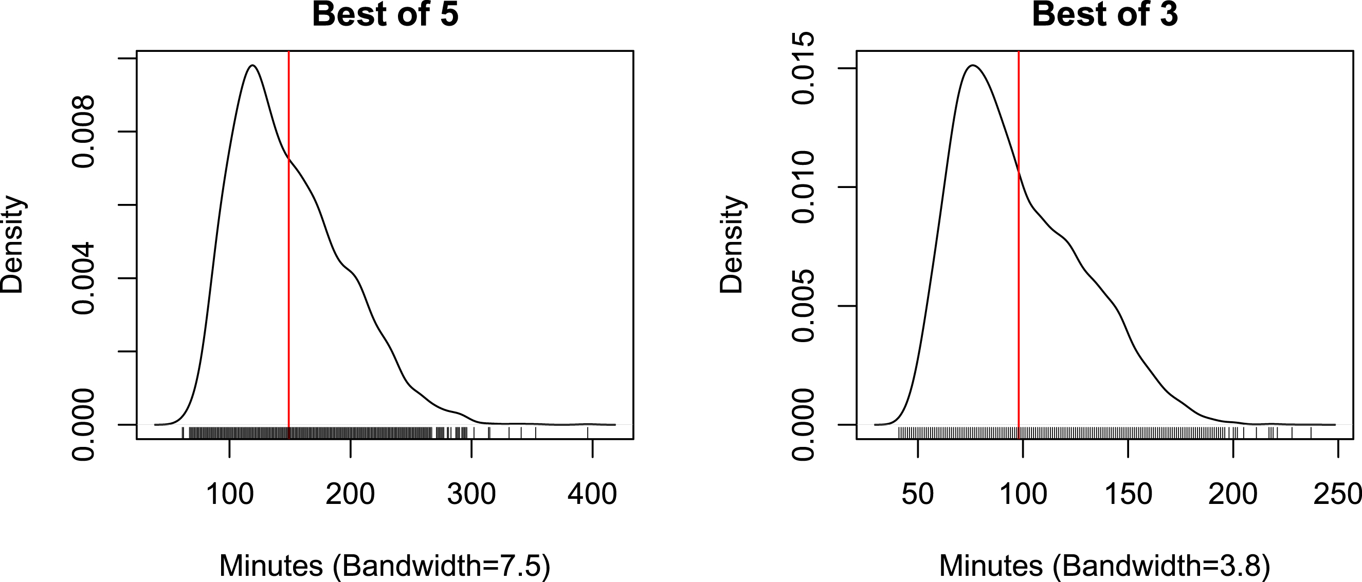
Table 1
Empirical quantiles for best of 3 and best of 5 matches duration (in minutes)
| Match | Q50 | Q75 | Q90 | Q95 | Q999 |
| Best of 3 | 92 | 119 | 142 | 154 | 200 |
| Best of 5 | 142 | 179 | 214 | 233 | 319 |
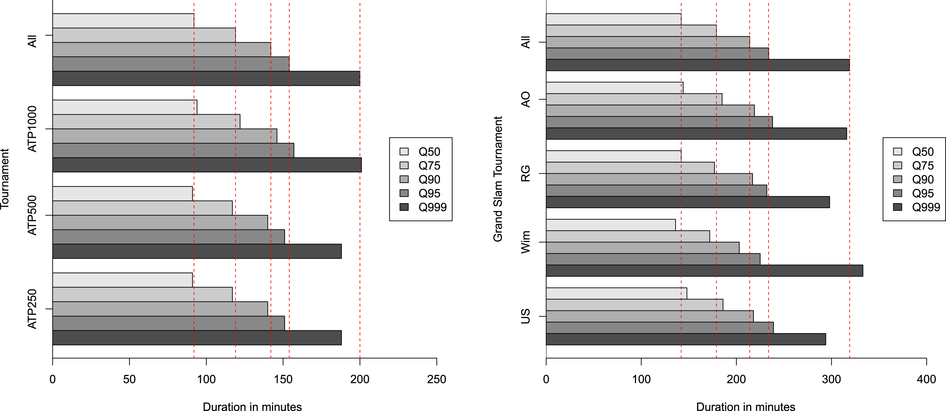
We now analyze durations with respect to different factors which have an impact on the length of a match. Figure 2 shows how durations’ quantiles change with respect to the type of tournament. The left panel, regarding best of 3 matches, suggests that ATP1000 matches are slightly longer than ATP500 and ATP250 matches, especially for extreme quantiles. This can be explained with the globally higher level of players taking part in ATP1000 tournaments and, thus, with more equilibrium between the two players in a match. The right panel refers to best of 5 matches and distinguishes durations with respect to Grand Slam championships. Results point out that Wimbledon matches have shorter durations than the other grand slam tournaments, except for the 99.9% quantile.
Fig. 2
Observed duration’s quantiles for best of 3 matches (left) and best of 5 (right).
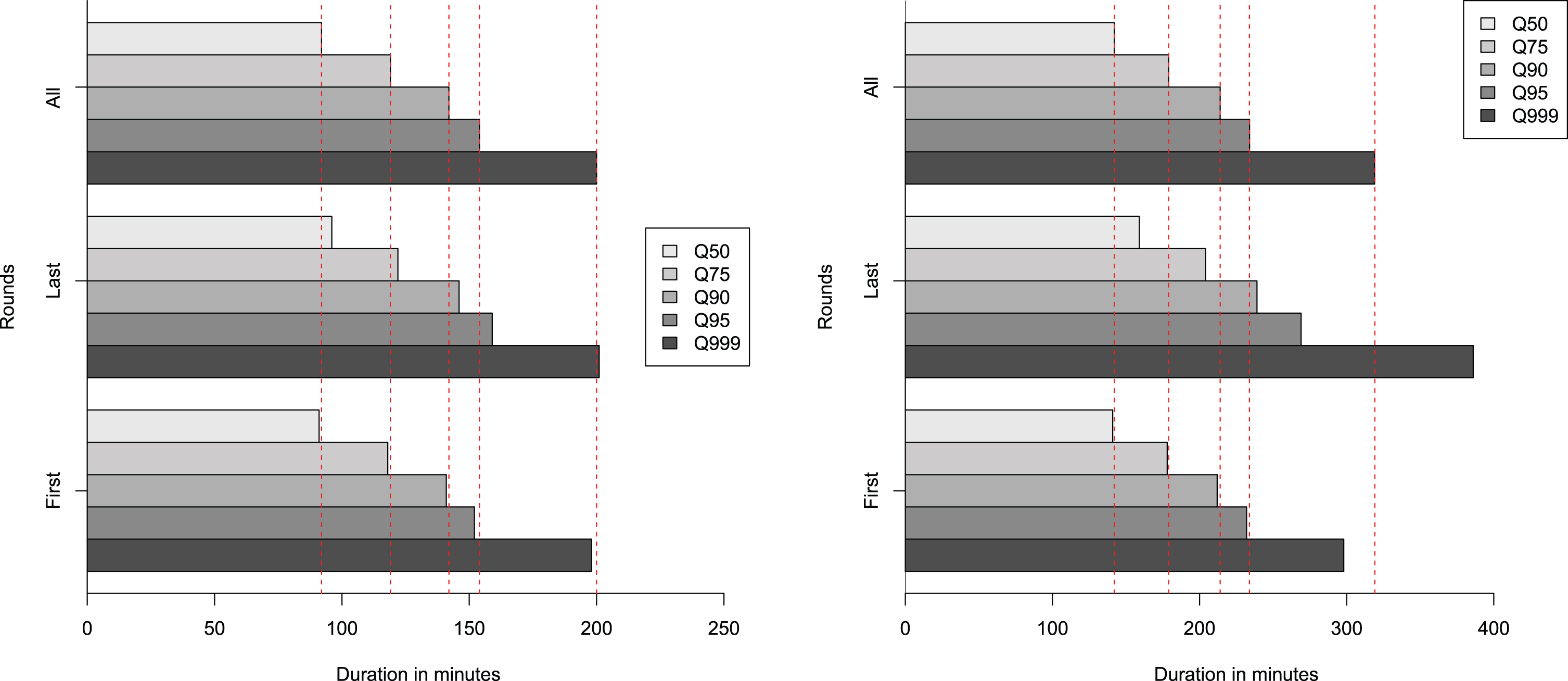
The effect of early rounds (up to eighth of final) and final rounds (from fourth of final) on matches’ durations is illustrated in Figure 3. Final rounds matches tend to be longer than those in early rounds, where often there is less equilibrium, especially for best of 5 matches.
Fig. 3
Observed duration’s quantiles for early and final rounds for best of 3 matches (left) and best of 5 (right).
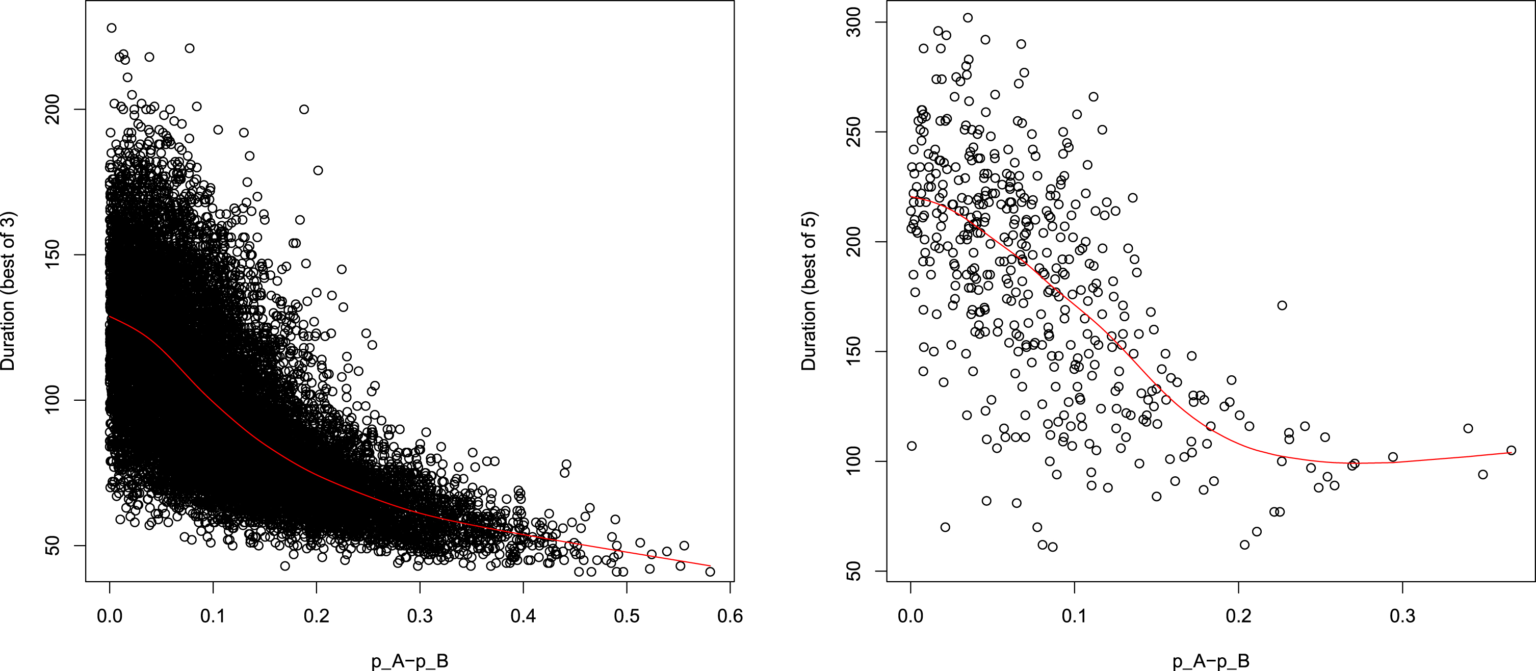
To further investigate this issue, following Klaassen and Magnus (2014), we considered the parameter δ = abs (pA - pB) as a measure of the level difference between players, where pA and pB are the probability that players A and B win a point on their own serve. Using the fraction of points won on serve as estimates of pA and pB, we performed a spline regression of durations on δ. Figure 4 shows the relation between the level difference (δ) and the duration: clearly the duration decreases non linearly with δ, that is when the match is less balanced.
Fig. 4
Relations between observed δ = abs (pA - pB) and durations for best of 3 matches (left) and best of 5 (right).
It clearly appears that a good simulator of matches’ length should include, directly or indirectly, all previous factors in the same proportions as they actually occur.
3Modeling and simulating tennis matches’ durations
In this section we show how to build a model for a realistic simulator of durations. The model is similar to the one proposed by Kovalchik and Ingram (2018), but not the same. In particular, it differs in that:
a) it does not require, and it never uses, Hawk-Eye data. This is a distinguishing feature of our model. While, in principle, using Hawk-Eye data would be preferable, it is not easy to find this kind of data and we believe that an approach based on publicly available data4 is more desirable for most users; b) it does not neglect time due to unusual match interruptions as well as the effect of exceeding the time prescribed by the International Tennis Federation’s rules; c) when simulating matches, it does not work with fixed probabilities of winning a point on serve, hence also γ = pA + pB and δ = pA - pB are not fixed. In particular, it resamples the “observed” pA and pB and, thus, γ and δ, over thousands of matches. This allows a better description of the actual variability of match conditions; d) since the final result of a match includes, in some way, the set of all conditions under which the match is played (temperature, humidity, hour of the day, indoor or outdoor, etc.) this, indirectly, allows us to account for all factors influencing its duration. In addition, since we resample real matches, each factor is weighted with the correct proportion (it occurs with the right frequency).
Among the “ingredients” previously described, we can distinguish between stochastic and deterministic factors. Elements necessary to simulate the in-play time are mainly stochastic, while those necessary to simulate between-play time can be deterministic or stochastic; time describing all the non standard interruptions will be treated by a suitable parameter.
3.1Modeling time in play
To simulate the in-play time we need to attribute a duration to each played point. For a given number of shots in a point, and using the well-known relation time = distance/speed, we estimate the time per point as the sum of time for each shot in that point. To replicate the physical mechanism leading to the duration of a single point we need to know the distributions of:
a) shots per point, to account for the variability of the number of shots;
b) the ball’s speed, to manage different speeds;
c) the distance covered by the ball, because it is not constant.
3.1.1Shots per point distribution
The distribution of the number of shots per point is the one suggested by Carboch et al. (2019), who analyzed in detail 24 matches played at the Australian Open, at Roland Garros and at Wimbledon. Matches were chosen to represent both early rounds and final rounds and were analyzed by three evaluators. Carboch et al. (2019) pointed out that most points end within the first three shots. These results are in line with those provided by the Match Charting Project (MCP)5, that gives categorized observed frequencies for 1–3 shots; 4–6 shots; 7–9 shots and 10 or more shots, on different surfaces.
The advantage of using the Carboch et al. (2019) distribution is that it provides the probability of a specific number of shots, instead of a categorized number of shots 6.
In their work, Carboch et al. (2019) produced observed frequencies of rally shots for different surfaces: clay, grass and hard. As the rally shots distribution for any specific surface is based on a limited number of matches (7 played at the Australian Open, 10 at the French Open and 7 at Wimbledon), to reduce the sample error, in our analyses we preferred not to differentiate among surfaces and consider a weighted mean of the observed frequencies over the three surfaces. We are very confident that this choice does not affect the final results. In addition, the maximum length of a rally was set at 30. The resulting rally shots distributions is represented in Figure 5 and listed in Table 2.
Fig. 5
Frequencies of rally shots obtained as a weighted mean of the frequencies provided by Carboch et al. (2019) for different surfaces.
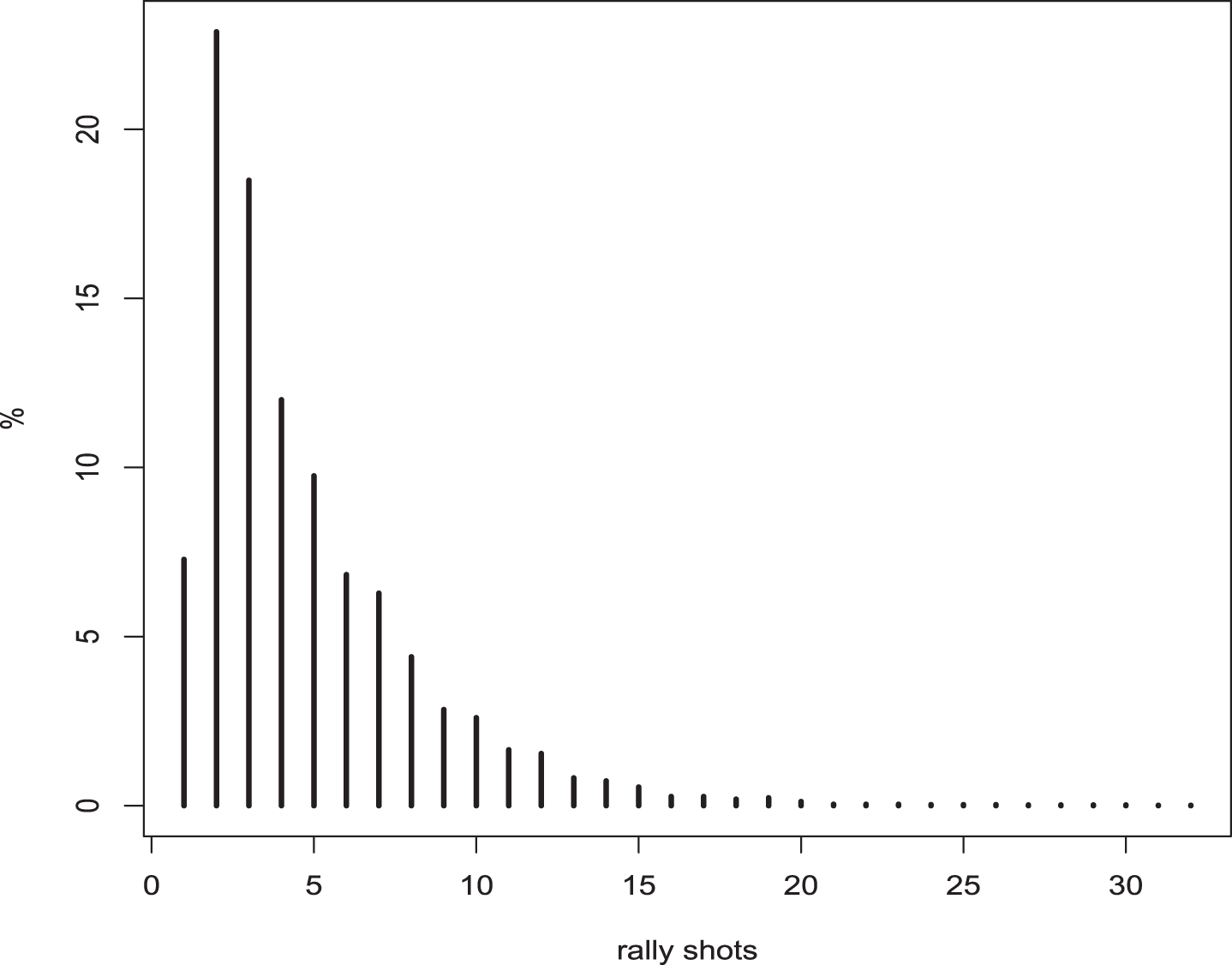
Table 2
Percentage frequencies of rally shots
| rally | 1 | 2 | 3 | 4 | 5 | 6 | 7 | 8 | 9 | 10 |
| Freq. | 7.28 | 22.88 | 18.49 | 12 | 9.75 | 6.83 | 6.28 | 4.40 | 2.84 | 2.60 |
| rally | 11 | 12 | 13 | 14 | 15 | 16 | 17 | 18 | 19 | 20 |
| Freq. | 1.65 | 1.54 | 0.83 | 0.73 | 0.55 | 0.27 | 0.27 | 0.19 | 0.12 | |
| rally | 21 | 22 | 23 | 24 | 25 | 26 | 27 | 28 | 29 | ≥ 30 |
| Freq. | 0.04 | 0.04 | 0.04 | 0.03 | 0.03 | 0.03 | 0.02 | 0.02 | 0.02 | 0.04 |
3.1.2Ball’s speed distribution
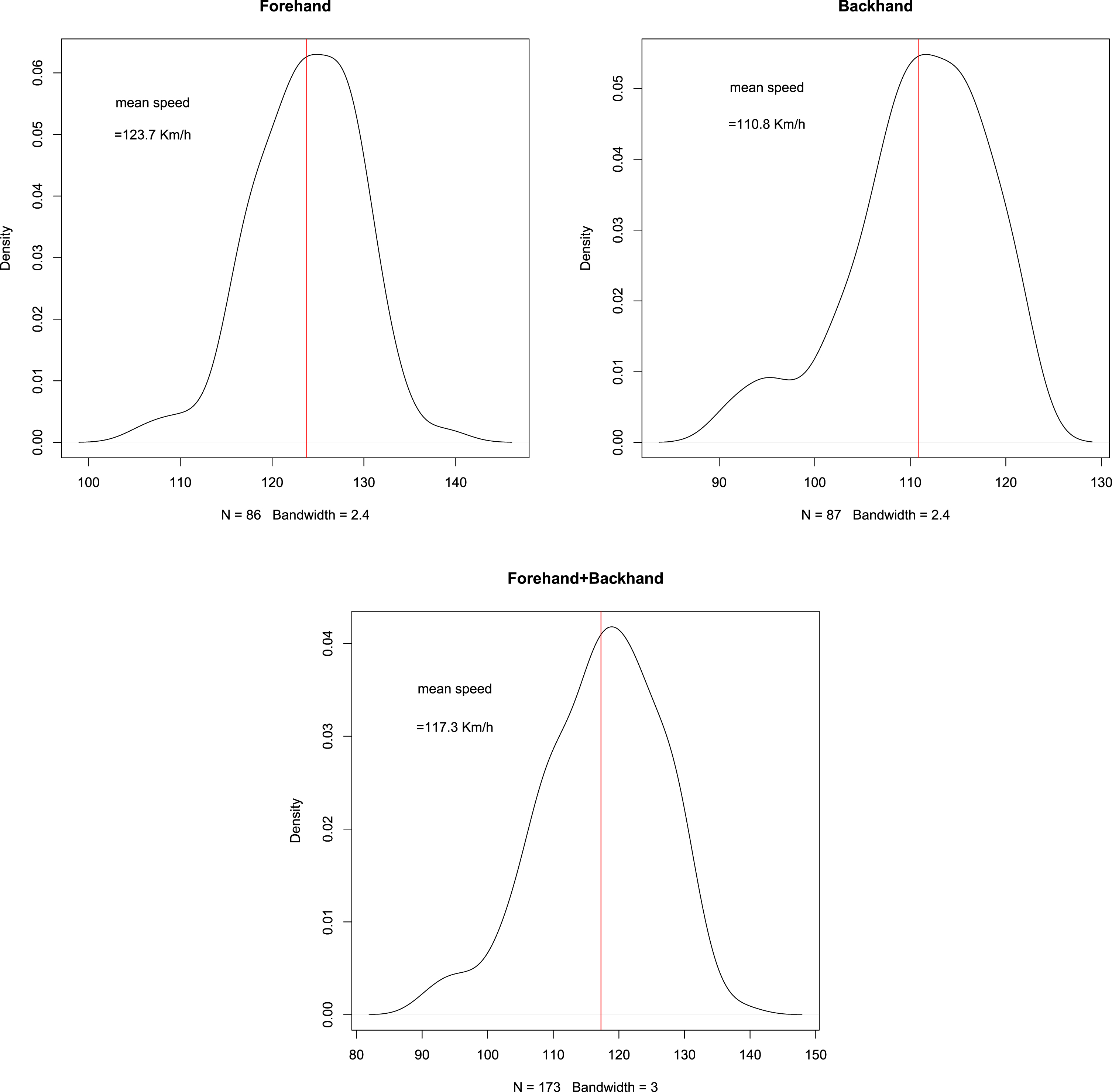
The distribution of the shots’ speed was estimated using data from some interactive graphs published in the blog on-the-T, containing median forehand7 and backhand8 speeds for 86 top players, measured by Tennis Australia’s Game Insight Group during the Australian Open tournaments, 2014 to 2016. In our simulations, data for forehands and backhands have been merged in order to obtain a unique distribution representing different speeds occurring in a match. Figure 6 shows the estimated kernel distributions for forehand, backhand, and both ground strokes. For forehand the median speed ranges from 106 to almost 140 km/h, with a mean around 123 km/h; backhands are usually slower: their speed ranges from 91 to 123 km/h with a mean of 110 km/h. When we consider the speed of both ground strokes the range is 91–139 km/h and the mean is 117 km/h.
Fig. 6
Ball’s speed distributions. From left to right: forehand speed, backhand speed, both ground strokes. Vertical lines show mean speeds.
3.1.3Distance covered by the ball
The length of a tennis court is 23.77m. On the one hand, diagonal and long shots can cover more than this distance and the ball’s trajectory is nonlinear; on the other hand, dropshots, volleys, passing shots and non-long shots, are sensibly shorter. Therefore, for the distance distribution we selected a N (23, 32). This means that the trajectory, at μ + 3 · σ, reaches the equivalent of 32 linear meters.
We tried other values for mean and standard deviation, but final results are not much affected by this choice. This is not surprising, given that at the mean speed of 117 km/h the ball takes 0.7 seconds to cover the 23.77 meters of the court’s length.
3.2Modeling time between play
For the time between play we can distinguish two components: time due to regular match interruptions, that we call regular time (RT), and time due to any other kind of interruptions, that we call additional time (AT). Regular time is made up of the time a player takes for 1st service and, if needed, for 2nd service preparation, changeovers and end of sets. The maximum durations of these interruptions are ruled by ITF: 20 seconds for first serve preparation9, 90 seconds for changeover and 120 seconds for end of set. We assume that players always use all the available time. Although the maximum length of the stops is ruled by ITF, a non trivial issue is the actual time a player uses for serve preparation and changeovers. Kovalchik (2018) showed that a professional tennis player takes, on mean, 19–20 seconds to serve but, in the meanwhile, she also showed that the mean time before a crucial point is around 25 seconds and can reach 40 seconds. The increasing time for serve preparation, when important points are involved, is supported also by the findings of Kolbinger et al. (2019). These authors, in a study considering 6231 rallies collected from 21 matches at the Australian Open 2016, indicated a mean time between points of 21.5 seconds with a standard deviation of 5.20 seconds. Hornery et al. (2007) found an average time of 25.1 seconds for matches played on hard court. According to the investigation of Périard et al. (2014), in hot conditions players take, on average, a 9.6 second longer break between points. Results in line with these findings were also pointed out by Carboch et al. (2019). As concerns the time rule violation, Kolbinger et al. (2019) found out that this occurs 58.8% of the times. Since long matches are usually very balanced, and balanced matches lead to several crucial points, we can safely assume that the occurrence of important points tends to increase with the length of the match. It is also reasonable to assume that in longer-lasting matches players are tired and tend to “nibble” some additional seconds between points. This suggests a possible link between the additional time required for serve preparation and the length of the match itself (see also Kolbinger et al. (2019) and Mühlberger and Kolbinger (2020)). Mühlberger and Kolbinger (2020) took a close look at the time between points in 18 matches at the 2018 men’s single US Open tournament after the introduction of an on-court serve clock to measure the time limit between points. Their conclusions are that, compared to previous studies, the number of rule violations decreased (26.3%) but the average time did not. They also confirm that players use time between points to recover after long rallies and show that umpires can have a significant influence on the inter-point time.
For these reasons, we model the time for first serve preparation as a Gamma random variable whose distribution is given by c + Gamma (a, b). For second serve preparation there is no “hard” time limit; according to Kovalchik and Ingram (2018), we fix it to 10 seconds. Parameters a, b and c have to be estimated. However, since we have no empirical data for this issue, we adopt an indirect strategy, consisting in choosing the parameters which lead to the best final result in terms of distance between the distributions of simulated and observed durations. Following this approach we model time for first serve preparation as 14 + Gamma(1.8, 0.305). To the best of our knowledge there are no data in the literature on changeover time violations. However, some measurements taken by the authors of this paper suggest that thresholds are often, and sometimes heavily, violated. Therefore, using the same approach as before, we model changeover time as 88 + Gamma(1.8, 0.275) and end-of-set time as 118 + Gamma(1.8, 0.275).
Additional time is more difficult to define and model. Exceedances of the previously defined times can be due to several reasons: exceedances of ruled time thresholds, but also, for example, Hawk-Eye calls. Each player has three unsuccessful challenges per set, with an additional challenge if the set reaches tie-break. If the player’s call is correct, then he/she retains the same number of challenges. Thus in a match there could be several calls, each one taking some time and, at the discretion of the umpire, some challenged points can be replayed. Some tennis analysts argue that players sometimes “tactically” call Hawk-Eye in order to gain time Kolbinger et al., 2019, Mühlberger and Kolbinger, 2020,and references therein. Random interruptions can also occur, due to medical time outs, audience bothering or moving, arbitration disputes, toilet breaks, heat time-outs and so on. There are also a number of possible unusual causes of interruptions, from ball boys hit by a ball to field invasion by animals or strikers.
It is clear that accounting for this additional time, which is neither constant nor imputable to a single specific cause, is not trivial. Thus we globally model AT as a parametric function of the simulated time passed since the beginning of the match (T0). In particular, we measure the additional time as AT = β log(T0), where β is a parameter that needs to be estimated. AT is added to the duration of the match obtained without accounting for any unexpected interruptions. The parameter β is estimated as the value minimizing the distance between the distributions of observed and estimated durations. The ratio behind this approach is to allow the simulation mechanism to adapt to the observed data without any attribution to a specific cause. The effect of this component was not accounted for by Kovalchik and Ingram (2018) but we found that its consideration significantly improves the fitting between simulated and observed durations, especially in the distributions’ tails.
3.3Matches simulations
To develop the match and, hence, to find the number of points, games and sets played, as well as the number of changeovers, we used Monte Carlo shot-level simulations (Newton and Aslam, 2006, 2009).
Even if this is the same approach followed by Kovalchik and Ingram (2018), the implementation of the model is quite different and, we believe, more appropriate. Indeed, Kovalchik and Ingram (2018) simulated matches only under some combinations of the quantities γ = pA + pB and δ = pA - pB (which they call bonus and malus). More in detail, for ATP matches they considered four values of δ (0.00, 0.05, 0.10 and 0.15) and three values of γ (1.20, 1.25 and 1.30 for hard and clay and 1.25, 1.30 and 1.35 for grass); then these values were further restricted to represent different round conditions. The authors declared that their values of γ and δ, “capture 95% of match conditions”. However, when we considered all the matches played in the period 2011–2018 and estimated the distribution of the “observed” (ex-post) values of δ (malus) and γ (bonus) we found the quantiles reported in Table 3. These quantiles suggest that the values used by Kovalchik and Ingram (2018) cover only around 89% of match conditions for best of 5 matches, and around 71% for best of 3 matches.
Table 3
Quantiles of observed γ and δ
| Best of 5 | Q1 | Q10 | Q30 | Q50 | Q70 | Q90 | Q99 |
| γ (bonus) | 1.051 | 1.134 | 1.205 | 1.249 | 1.298 | 1.360 | 1.478 |
| δ (malus) | 0.002 | 0.014 | 0.041 | 0.068 | 0.097 | 0.157 | 0.284 |
| Best of 3 | Q1 | Q10 | Q30 | Q50 | Q70 | Q90 | Q99 |
| γ (bonus) | 1.008 | 1.129 | 1.214 | 1.272 | 1.329 | 1.415 | 1.529 |
| δ (malus) | 0.002 | 0.021 | 0.060 | 0.100 | 0.148 | 0.231 | 0.366 |
| All together | Q1 | Q10 | Q30 | Q50 | Q70 | Q90 | Q99 |
| γ (bonus) | 1.008 | 1.129 | 1.214 | 1.271 | 1.328 | 1.414 | 1.529 |
| δ (malus) | 0.002 | 0.021 | 0.059 | 0.099 | 0.147 | 0.230 | 0.365 |
To build our model, instead, we used probabilities that: player A (B) wins a point on his own service given that the first service is in; the first service of player A (B) is in; player A (B) wins a point on his second service given that the second service is in; the second service of player A (B) is in. These probabilities have been estimated using 20,096 matches played between 2011 and 2018, whose statistics are provided by the On court database10. Table 4 lists means, across all matches, of the estimated probabilities, divided also for surface.
Table 4
Means of the estimated probabilities for different surfaces.
| Probab. | Hard | Clay | Grass | Tot |
| P(1st serve in) | 60.0 | 61.6 | 62.4 | 60.7 |
| P(2nd serve in) | 88.5 | 90.1 | 86.4 | 88.8 |
| P(Point won on 1st serve ∣ 1st serve in) | 72.6 | 69.0 | 74.1 | 72.0 |
| P(Point won on 2nd serve ∣ 2nd serve in) | 56.8 | 55.6 | 58.1 | 56.5 |
| P(Point won on 1st serve) | 43.5 | 42.5 | 46.2 | 43.4 |
| P(Point won on 2nd serve) | 51.3 | 50.7 | 52.2 | 51.2 |
For each simulated match, the set of model’s parameters (probabilities) is sampled from the ones characterizing the observed matches. This allows us to capture 100% of the match conditions, in terms of differences between players and with respect to weather conditions, kind of tournament, round, etc. In addition, given that we resample observed matches, all these features are weighted in the correct way.
A step by step description of the simulation procedure is given in the Appendix.
4Simulation results
This section is devoted to an in-depth analysis of the coherence between simulated and observed matches’ lengths. A description of time components is also provided.
Table 5 lists the simulated quantiles and means, with their Monte Carlo intervals, and the corresponding observed values for Bof3 and Bof5 matches played in 2011–2018.
Table 5
Observed and simulated quantiles and means for Bof3 and Bof5 matches durations (in minutes), with their 95% Monte Carlo intervals in parentheses. Note that all values referring to simulated matches are rounded to the nearest minute. Sample size: 16246 for Bof3 and 3715 for Bof5 matches
| Best of 3 | Q2.5 | mean | Q97.5 | Q99.0 | Q99.9 |
| Observed | 54 | 98 | 164 | 175 | 200 |
| Simulated | 54 | 98 | 166 | 179 | 208 |
| (53–55) | (97–98) | (164–168) | (174-184) | (203–219) | |
| Best of 5 | Q2.5 | mean | Q97.5 | Q99.0 | Q99.9 |
| Observed | 84 | 150 | 253 | 274 | 319 |
| Simulated | 84 | 150 | 254 | 275 | 324 |
| (83–85) | (150–151) | (251–256) | (272–279) | (316–332) |
To account for the variability in simulations, the α-quantile for simulated data refers to the mean of 500 α-quantiles, each one computed over 15000 simulated matches. The 500 values for each α-quantile allow us to compute the 95% Monte Carlo intervals both for the mean and for the the quantiles, written in parentheses in Table 5. The 2.5% percentile and the mean are correctly estimated in both cases and the errors for the 97.5% percentiles are +2 minutes, for Bof3, and +1 minute, for Bof5 matches. For higher-order quantiles, i.e. 99.0% and 99.9% quantiles, the model overestimates the “observed” percentiles by +4 and +8 minutes for Bof3 matches, and by +1 and +5 minutes for Bof5 matches. Up to quantile 97.5% Monte Carlo intervals are quite narrow and, as usual, moving towards the right distribution’s tail, they become larger.
These results show a very good fit, especially if compared with the results obtained with the model by Kovalchik and Ingram (2018) which – according to the values published in their paper – underestimates the 97.5% actual percentile by 12 minutes for Bof3 matches and by 24 minutes for Bof5 matches and, in the meantime, overestimates the 2.5% percentile by 7 minutes both for Bof3 and Bof5 matches.
4.1Goodness-of-fit of the model
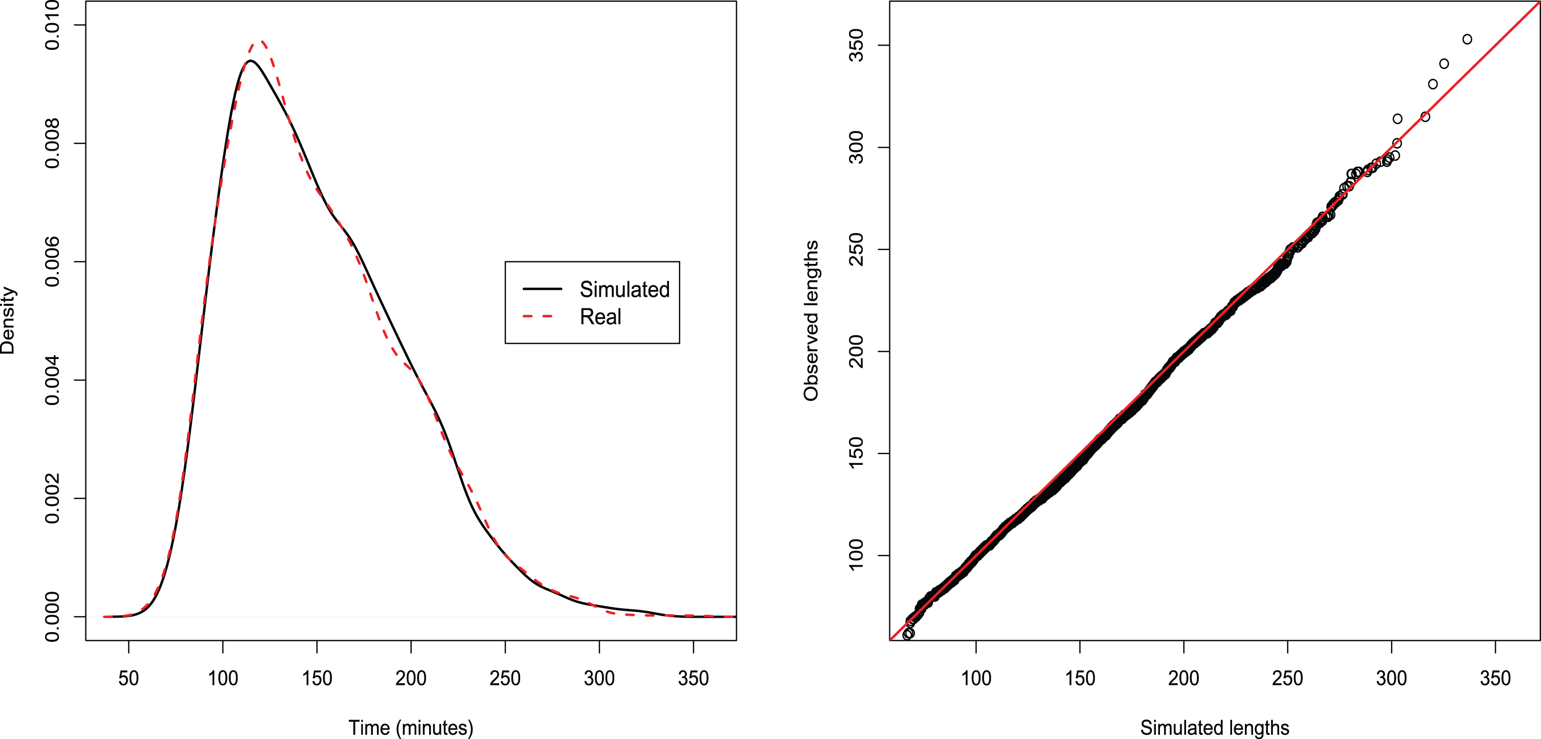
Simulated distributions of matches’ lengths (see Figs. 8 and 9) are now compared with the observed ones using graphical representations as well as statistical tests. Analyses are conducted separately for best of 3 and best of 5 matches.
Fig. 8
Best of 3: distributions and QQ-plots. Tests’ p-values: KS=0.08, AD=0.33, FP=0.54.
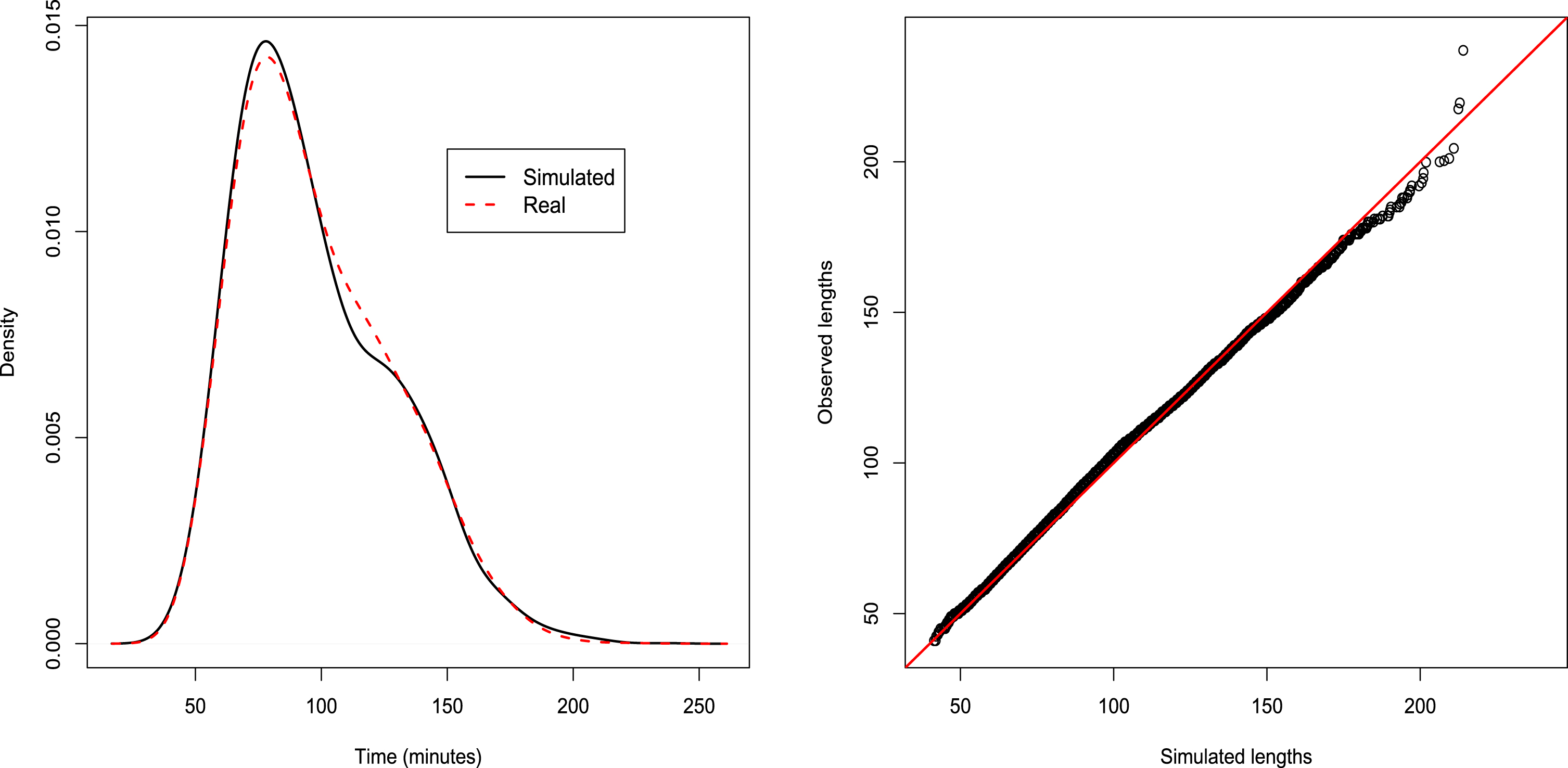
Fig. 9
Best of 5: distributions and QQ-plots. Tests’ p-values: KS=0.47, AD=0.42, FP=0.75
Let us denote by Dobs and Dsim the observed and simulated distributions of a match length. To test H0 : Dobs = Dsim we consider several statistical methods of goodness-of-fit that we can roughly divide into four categories:
1) graphical methods, such as graphs of the density distributions and their QQ-plot;
2) a statistical test based on permutations, i.e. the Fisher-Pitman (FP) test (e.g. Hollander and Wolfe, 1999). This test mainly considers the center of the distribution while giving less importance to tails because the null hypothesis of equality is tested only against shift alternatives;
3) tests based on the distance between the CDF’s. They consider all the quantiles of the distributions and, thus, give more relevance to the tails. The two-sample Kolmogorov-Smirnov (KS) test (e.g. Conover, 1971, pp. 309–314) and the Anderson-Darling (AD) test Scholz and Stephens, 1987 belong to this category. The Anderson-Darling test is generally more powerful than the Kolmogorov-Smirnov test Razali and Wah, 2011; while the former is more sensitive to the tails of the distribution, the latter is more aware of the distribution center;
4) methods focusing only on the distribution tails and giving less importance to the central part of the distribution. They refer to the extreme value theory (EVT) and are based on the comparison between the tail parameters of the two distributions.
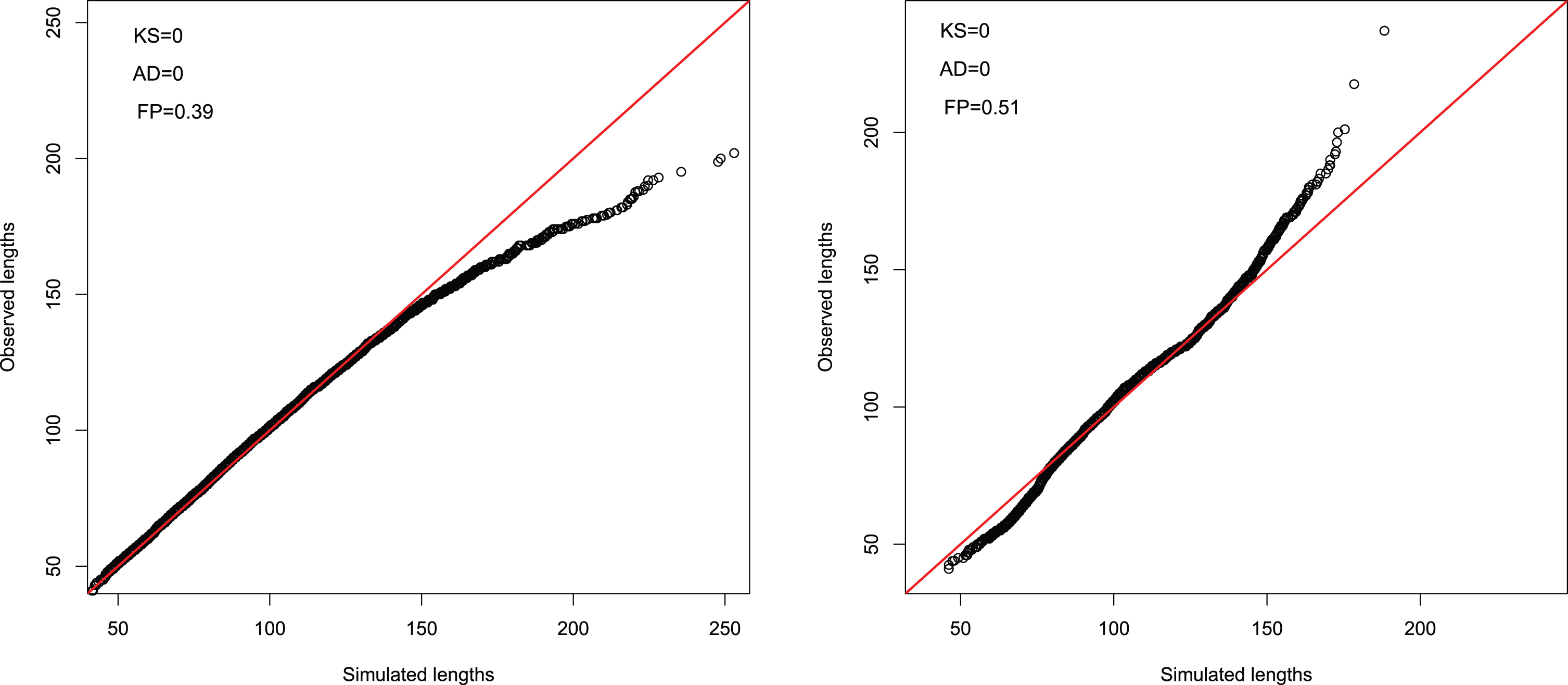
Before applying these methods, we want to stress that a suitable evaluation of goodness-of-fit requires to specifically account for the tail behavior of the distribution. Figure 7 shows two examples of QQ-plots for which the FP test fails to reject the null hypothesis, while the KS and AD tests largely reject it. Looking at the left panel of Figure 7, it is clear that the two distributions are almost identical in the left tail and in the central part, but strongly differ in the right tail; similarly, in the right panel example, in spite of a generally inadequate fitting, especially in the tails, the fitting in the central part of the distribution is sufficient for the FP test not to reject the null hypothesis at the 5% confidence level.
Fig. 7
Examples of QQ-plots for which the FP test does not reject while the KS and AD tests do.
The application of the Kolmogorov-Smirnov, Anderson-Darling and Fisher-Pitman tests to simulated and observed distributions leads to the following p-values: pKS = 0.09, pAD = 0.19 and pFP = 0.77 for Bof3 matches and pKS = 0.64, pAD = 0.61 and pFP = 0.97 for Bof5 matches. Clearly, the hypothesis of equal distributions is not rejected at the usual 5% significance level11.
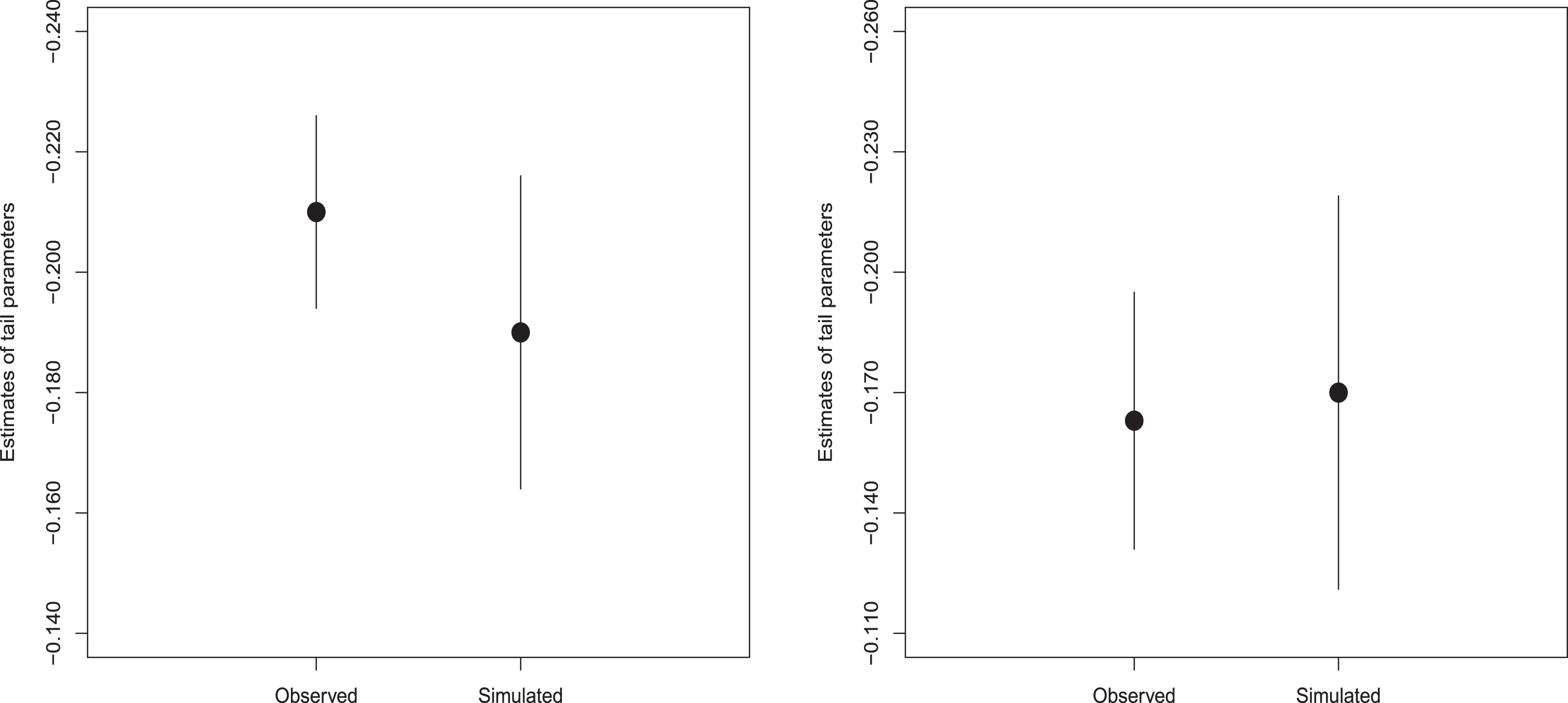
The estimation of the tail parameters of the distributions has been performed using the so-called peak-over-threshold method within the extreme value theory framework (see e.g. Coles, 2001). The analysis of the mean excess plot suggested to fix the threshold to 120 minutes for Bof3 matches and to 180 minutes for Bof5 matches. Maximum likelihood estimates of the tail parameter ξ for simulated and observed data are
Fig. 10
Estimates of the tail parameters (ξ) for observed and simulated Best of 3 and Best of 5 matches. Bof3 matches:
This in-depth analysis of goodness-of-fit allows us to conclude that our model leads to an extremely realistic simulation of tennis matches’ durations, also for quite long matches.
4.2Time components analysis
Given that our simulation model works well and coherently with the observed durations, we can now analyze the time components of a match. All the following considerations are based on the mean results over 50, 000 simulated matches.
Figure 11 shows the percentage components of time in a match. Within our framework, the effective playing time amounts to 9.6% for Bof3 matches and 10.5% for Bof5 matches. Thus time between play takes around 90% of the total length of a match. The effective playing time reported in literature is usually greater and ranges from around 10 to around 30% of the total time of a match, see for example Smekal et al. (2001), Morante and Brotherhood (2005), Kovacs (2006), Fernandez et al. (2006), Mendez-Villanueva et al. (2007), Kilit et al. (2016). However, in the literature, studies are quite heterogeneous with respect to methods, experimental conditions and results. Some works are based only on few matches (10 in Smekal et al., 2001, 39 in Morante and Brotherhood, 2005) or few players (20 in Smekal et al., 2001, 8 in Mendez-Villanueva et al., 2007, 10 in Kilit et al., 2016); others are not based on real matches (in Smekal et al., 2001, each match lasts 50 minutes, in Kilit et al., 2016, simulated tennis matches last one hour); others refer to players of a quite different level (Smekal et al., 2001, consider players without ATP ranking, Kilit et al., 2016, consider players with ATP ranking between 800 and 1600; some references in Fernandez et al., 2006, take into account a national or regional level, Kovacs, 2006, a college level). Even more importantly, some authors explicitly declare that the effective playing time was determined by dividing the entire playing time of a game by the real playing time performed in a specific game, without including breaks, see Mendez-Villanueva et al. (2007), Kilit et al. (2016), Smekal et al. (2001).
Fig. 11
Percentage time components for Bof3 and Bof5 matches. 1st serve: time for 1st serve preparation; 2nd serve: time for 2nd serve preparation; changeover: time for changeovers and end of sets; other: time for any other kind of interruption.
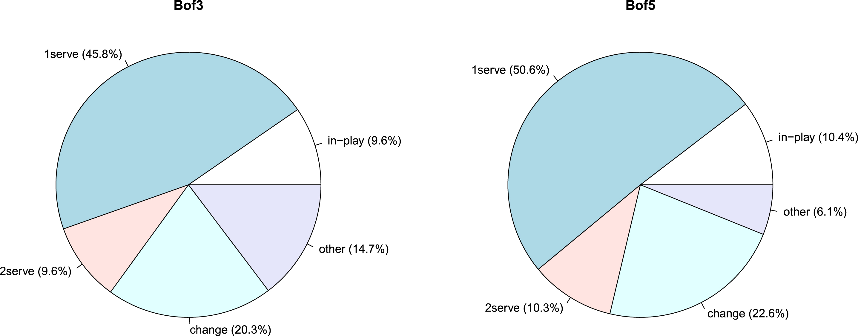
The time required for serve preparation amounts, globally, to 55.4% for Bof3 matches and 60.9% for Bof5 matches. Changeovers and end of sets take around 20 - 22% of the total time. It is interesting to note that the additional time component (AT, Other) takes a non negligible fraction: 14.7% for Bof3 matches and 6.1% for Bof5 matches, and this is important for the description of actual durations. As a proof of this, the model by Kovalchik and Ingram (2018), which simply assumes that players use only all the ruled time, both for serve preparation and for changeovers, significantly underestimates the actual high-order quantiles. As the occurrence and duration of some unusual events do not directly depend on the number of sets or games, it is not strange that the percentage impact of these events is higher for Bof3 matches. For example, a three-minute medical time-out weighs around 3% on the mean duration of a Bof3 match and around 2% on the mean duration of a Bof5 match. However, in absolute terms, and with respect to mean durations, the AT component lasts, on average, around 9 minutes for Bof5 matches and around 14 minutes for Bof3 matches. This finding is bizarre because one could expect that the longer the match, the more likely the occurrence of some unusual event. We have no clear explanation for this issue yet and, thus, it will need more analyses in the future.
5Case studies
Having proved that our model works well and correctly fits the data, we used it to perform three different applications. The first is about formats reducing the probability of long matches without impacting too much on the current match setting. The second and third applications concern new rules for tie-break in the fifth set at Wimbledon and the opportunity to introduce tie-break in the fifth set at Roland Garros.
5.1Abolishing first service or advantages
The Fast4 format, which is currently experimented at the Next gen ATP finals, clearly reduces the matches’ length but has a strong impact on the whole architecture of the match and is often perceived by players and audience as “another sport”. Our goal, instead, is to experiment formats which, while reducing the probability of very long matches, preserve the normal structure of sets.
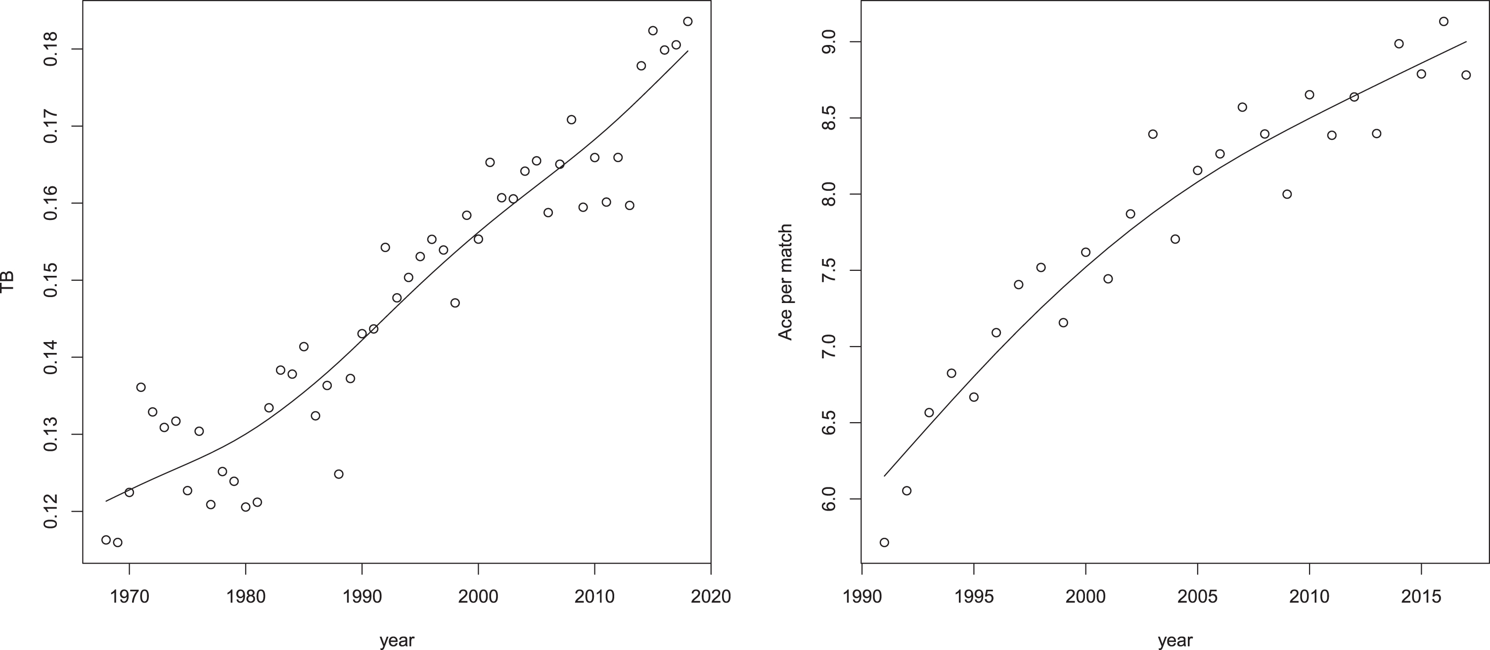
Let us consider Figure 12. The left panel shows the evolution of the ratio, TBt, between the number of sets requiring at least 12 games and the number of sets played in year t. The right panel shows the mean number of aces per match in each year for the first 100 top players. The red lines are kernel estimates of the relation. Both graphs are monotonically increasing. While at the beginning of 1990s one set in seven finished 7-5 or 7-6, now the same occurs in one set in five, with the mean number of aces per match increased from the almost six in the 1990s to the current nine. One of the reasons for this increase is the technological improvement in rackets and strings, which allows to serve faster.
Fig. 12
Left panel: time evolution of the ratio between the number of sets requiring at least 12 games and the number of sets played in a year (TBt); right panel: time evolution of the mean number of aces per match in a year. The red lines are kernel estimates of the relation between the variable and the time. Source: www.atptour.com
These graphs help to understand that a shorter duration of matches, without impacting on the sets structure, may be achieved by breaking the equilibrium and reducing the service dominance. To reach this goal both the abolition of the advantages on 40-40 (also called sudden death or killer point) and the abolition of the second serve could be effective Magnus and Klaassen, 2000. However no single matches are actually played with only these limitations. Thus, to evaluate their impact we resort to simulations. In particular, while the abolition of the advantages has been considered by Kovalchik and Ingram (2018), the abolition of the second serve has never been studied using simulations. Yet, this option has been proposed several times since the 1920s, because there is no particular reason why the player at serve should have two possibilities and because no other sport has such a rule. Nevertheless, it has never been applied.
To simulate a match with only one serve we have to imagine the consequences of abolishing the two-service rule in terms of serve performance. In this work we follow the view of Klaassen and Magnus (2014): a player with only one service is equivalent to a player with two services who has fault the first one. Thus, we use data referring to the current second service and to model’s parameters. This is also why we use the expression ‘abolishing the first service’ instead of ‘abolishing the second service’.
In our simulations we compare four formats:
- the standard format, providing for matches played best of 5 or best of 3, with 2 services, advantages on 40-40, and a 7 point tie-break on 6-6 in all sets;
- the standard format played with only one service;
- the standard format played with no advantages on 40-40;
- the standard format with no advantages and one service.
Results, in terms of median durations and probabilities of a match lasting more that k hours, are given in Table 6. They are based on 20,000 matches played best of 5. The model’s parameters have been estimated using only data from grand slams’ championships.
Table 6
Median durations (in minutes) and percentage probabilities of a match lasting more that k hours under different formats
| Best of 5 | ||||||
| Scenario | Median | P (>3) | P (>3.5) | P (>4) | P (>4.5) | |
| Standard | 144 | 25.2 | 10.6 | 3.5 | 1.2 | |
| No Ad | 132 | 15.0 | 4.7 | 1.3 | 0.4 | |
| One service | 114 | 10.1 | 3.5 | 0.9 | 0.2 | |
| No Ad &One service | 106 | 4.4 | 0.9 | 0.3 | 0.05 | |
Results show that both the ‘No Ad’ and ‘One service’ options are effective in reducing the probability of matches lasting more than three hours, with a stronger effect produced by the ‘one service’ format. The effect is even more drastic if both modifications are introduced, with a 4.4% probability of exceeding 3 hours. Apart from the duration itself, it is known that shorter formats also imply an increase in the number of upsets (for instance, Kovalchik and Ingram, 2018) and, thus, in the uncertainty about the final result of the match.
5.2Tie-break at Wimbledon
In 2019, for the first time, tie-break was introduced in the fifth set at Wimbledon. However it was not played at 6-6 but at 12-12. Although from this new rule a very marginal impact is expected on match durations, we try to quantify it and compare its impact with that of a standard 7-point tie-break at 6-6.
It is clear that, here, we are not considering emotions and thrill of matches arriving, for example, at 12-12 in the fifth set, can produce.
To replicate as much as possible the features of matches at Wimbledon, in the simulations all parameters are fixed using only matches played at Wimbledon in the past.
Median durations and percentage probabilities of a Wimbledon match lasting more than k hours are listed in Table 7. It is clear that a tie-break at 12-12 has no practical effects on most matches and, on average, has limited effects also on long matches. For example, the percentage probability of a match lasting more than six hours is 0.86 with no tie-break, 0.71 with a tie-break at 12-12 and 0.68 with a tie-break at 6-6. While this avoids extremely long matches like the Isner-Mahut match at Wimbledon 2010, it does not prevent the occurrence of long matches like the final played at Wimbledon 2019 by Federer and Djokovic.
Table 7
Impact of the introduction of tie-break in the fifth set at Wimbledon at 6-6 and at 12-12
| Wimbledon | |||||||
| Scenario | Median | P (>3) | P (>3.5) | P (>4) | P (>4.5) | P (>5) | |
| No TB (up to 2018) | 151 | 31.7 | 18.2 | 9.6 | 5.0 | 2.6 | |
| 5th set TB (12-12) | 150 | 31.2 | 16.8 | 8.7 | 4.5 | 2.7 | |
| 5th set TB (6-6) | 150 | 31.2 | 16.8 | 8.5 | 4.2 | 2.0 | |
5.3The introduction of tie-break at Roland Garros
Currently, the French Open is the only Grand Slam tournament without tie-break in the fifth set. What would be the consequences of introducing it? Again, we compare the actual format with one in which a 7-point tie-break is played at 6-6 in the fifth set. Also in this case, all parameters are set using only matches played at Roland Garros.
Median durations and percentage probabilities of a Roland Garros match lasting more that k hours are listed in Table 8. Tie-break has some effects on matches lasting at least 3.5 hours. The impact is not dramatic, although the percentage probability of matches lasting more than 5 hours decreases from 3.2 to 2.5 and that of lasting more than 6 hours from 1.2 to 0.8.
Table 8
Impact of the introduction of tie-break in the fifth set at 6-6 at Roland Garros
| Roland Garros | ||||||
| Scenario | Median | P (>3) | P (>3.5) | P (>4) | P (>4.5) | P (>5) |
| Current | 154 | 34.12 | 19.4 | 10.3 | 5.4 | 3.2 |
| 5th set TB (6-6) | 154 | 34.2 | 19.0 | 9.8 | 4.7 | 2.5 |
6Conclusions
In this paper, observed durations of male tennis matches have been analyzed under different viewpoints and a procedure to simulate them has been developed. The comparison between distribution of observed and simulated durations show that this approach is able to reproduce the observed features of the durations’ distribution.
Our procedure has three distinguishing features. First, it considers durations in terms of actual time rather than played points.
Secondly, in the simulations we resampled empirical characteristics of observed matches (probabilities of winning a point on serve, of winning a point on first or second serve, percentages of first and second serves, etc.). As resampled parameters are related to all sampled matches and these are played under different conditions (surfaces, tournament type, earlier and final rounds, weather conditions, etc.), this allows a complete and realistic description of the actual complexity.
Thirdly, we introduced a time component designed to account for unexpected interruptions (medical time outs, Hawk-Eye calls, audience bothering, etc.) as well as violations of the prescribed time between points, serves and games. The consideration of this component permits a much better approximation of the right tail in the observed length distribution.
Particular attention has been paid to the analysis of the goodness-of-fit of the simulated distributions and their coherence with the observed ones. These analyses suggest that our model provides an accurate description not only of the central quantiles of the actual length distribution but also of the low-order and high-order quantiles, that is of the shortest and, most importantly, longest matches’ length.
The whole procedure requires the estimation of the distribution of several variables in order to simulate partial times. Some of them are not directly estimated from observed data, for example the distributions of times between two points or between changeovers or the distribution of the distance covered by the ball in a shot. Also the choice of the function describing the additive time accounting for unexpected interruptions is, in some way, subjective. Indeed, other functions, for example a logistic function of the total time, could have been used with similar results. The main reason for this subjectivity is the lack of information about the involved features; in this sense these choices can be viewed as a limit of our study. On the other hand, all the different distributions with their parameters and the function for the additive time can be considered as a sort of “hyper-parameter” which needs to be adapted in order to best describe what has been observed. As the “hyper-parameter” was chosen in order minimize the discrepancy between the distributions of the observed and simulated durations, the latter can be thought of as based on the data, although indirectly.
The investigation of the different time components reveals that over 90% of time in a match is spent when the ball is not in play, and that there are evidences that the maximum lengths of interruptions ruled by ITF are often exceeded. The latter result is in line with the findings of Carboch et al. (2019), Kolbinger et al. (2019) and Mühlberger and Kolbinger (2020).
The present research has certainly some limits. In this paper we focused only on matches’ durations without analyzing the impact of changes in the rules on other characteristics, for example on the average excitement per point or on expected upsets (Pollard and Barnett, 2018).
Only men’s matches have been considered here; a similar analysis for female matches and a suitable comparison would be surely interesting.
It could be argued that non standard interruptions may be tournament dependent: for example, heat time-out is present only at the Australian Open, on clay there is no Hawk-Eye (which does not mean there aren’t challenges!), at Wimbledon audience is usually less noisy than at the US Open, and so on. Even if, globally, all these causes tend to compensate each other so that a mean effect is enough for a good fitting, it could be interesting to apply this model to specific tournaments and to study possible differences.
A not completely satisfying issue of this paper is the additive component; while it works well to evaluate the distribution of durations, the fact that it is greater for Bof3 matches than for Bof5 matches is bizarre and unexpected. At the moment we have no explanation but this point requires further analyses to reach a clear interpretation.
More generally, the whole procedure will benefit from the availability of data allowing more accurate estimates of the components (time between points and between changeovers, speed of the ball, distance covered by the ball, shot rally distribution, unexpected interruptions) generating the total duration of a match.
Conditionally to these limits we have also provided a description of how the probability of a long match changes due to modifications of the current format. For example, the probability of a best of 5 match lasting more than three hours is around 25% with the current format, but it can possibly reduce to around 15% by the abolition of advantages on 40-40 and to around 10% by the abolition of the first serve. Of course, these findings should be proved and verified in real matches. Finally, we have quantified the effects of the new tie-break’s format at Wimbledon and of the possible introduction of tie-break at Roland Garros.
References
1 | Barnett, T. , (2016) , A recursive approach to modeling the amount of time played in a tennis match, Medicine & Science in Tennis, 21: , 27–35. |
2 | Barnett, T. , Brown, A. and Pollard, G. , (2006) , Reducing the likelihood of long tennis matches, Journal of Sport Science and Medicine, 5: , 567–574. |
3 | Betensky, R. , (2019) , The p-value requires context, not a threshold, The American Statistician, 73: , 115–117. |
4 | Carboch, J. , Siman, J. , Sklenarik, M. and Blau, M. , (2019) , Match characteristics and rally pace of male tennis matches in three grand slam tournaments, Physical Activity Review, 7: , 49–56. |
5 | Carboch, J. , Vejvodova, K. and Suss, V. , (2016) , Analysis of errors made by line umpires on ATP tournaments, International Journal of Performance Analysis in Sport, 16: (1), 264–275. |
6 | Chatfield, C. , (1995) , Problem Solving: A Statistician’s Guide, 2nd ed., Chapman & HallCRC. |
7 | Coles, S. , (2001) , An Introduction to Statistical Modeling of Extreme Values, Springer. |
8 | Conover, W. J. , (1971) , Practical Nonparametric Statistics, John Wiley & Sons. |
9 | Fernandez, J. , Mendez-Villanueva, A. and Pluim, B. M. , (2006) , Intensity of tennis match play, British Journal of Sports Medicine, 40: (5), 387–391. |
10 | Ferrante, M. , Fonseca, G. and Pontarollo, S. , (2017) , Howlong does a tennis game last?, in Proceedings of MathSport International 2017 Conference, pp. 122-130, Padova University Press. |
11 | Hollander, M. and Wolfe, D. A. , (1999) , Nonparametric Statistical Methods, John Wiley & Sons. |
12 | Hornery, D. J. , Farrow, D. , Mujika, I. and Young, W. , (2007) , An integrated physiological and performance profile of professional tennis, British Journal of Sports Medicine, 41: (8), 531–536. |
13 | Kilit, B. , Senel, O. , Arslan, E. and Can, S. , (2016) , Physiological responses and match characteristics in professional tennis players during a one-hour simulated tennis match, Journal of Human Kinetics, 51: , 83–92. |
14 | Klaassen, F. and Magnus, J. , (2014) , Analyzing Wimbledon. The Power of Statistics, Oxford University Press. |
15 | Kolbinger, O. , Großmann, S. and Lames, M. , (2019) , A closer look at the prevalence of time rule violations and the inter-point time in men’s grand slam tennis, Journal of Sport Analytics, 5: (2), 75–84. |
16 | Kovacs, M. S. , (2006) , Applied physiology of tennis performance, British Journal of Sports Medicine, 40: (5), 381–386. |
17 | Kovalchik, S. A. , (2018) , Why the tennis “serve clock” may be a waste of time, Significance, 15: (4), 36–39. |
18 | Kovalchik, S. A. and Ingram, M. , (2018) , Estimating the duration of professional tennis matches for varying formats, Journal of Quantitative Analysis in Sports, 14: (1), 13–23. |
19 | Magnus, J. and Klaassen, F. , (2000) , How to reduce the service dominance in tennis? Empirical results from four years at Wimbledon, Technical report, Tilburg University, School of Economics and Management. |
20 | Mendez-Villanueva, A. , Fernandez-Fernandez, J. , Bishop, D. , Fernandez-Garcia, B. and Terrados, N. , (2007) , Activity patterns, blood lactate concentrations and ratings of perceived exertion during a professional singles tennis tournament, British Journal of Sports Medicine, 41: (5), 296–300. |
21 | Morante, S. and Brotherhood, J. , (2005) , Match characteristics of professional singles tennis, Medicine & Science in Tennis, pp. 12-13. |
22 | Mühlberger, A. and Kolbinger, O. , (2020) , The serve clock reduced rule violations, but did not speed up the game: A closer look at the inter-point time at the 2018 us open, Journal of Human Sport and Exercise, in press, DOI: https://doi.org/10.14198/jhse.2021.163.05. |
23 | Newton, P. and Aslam, K. , (2006) , Monte Carlo tennis, SIAM Review, 11: (3), 722–742. |
24 | Newton, P. and Aslam, K. , (2009) , Monte Carlo tennis: A stochastic Markov chain model, Article, Journal of Quantitative Analysis in Sports, 5: (3), Article 7. |
25 | Périard, J. D. , Racinais, S. , Knez, W. L. , Herrera, C. P. , Christian, R. J. and Girard, O. , (2014) , Thermal, physiological and perceptual strain mediate alterations in match-play tennis under heat stress, British Journal of Sports Medicine, 48: , i32–i38. |
26 | Pollard, G. and Barnett, T. , (2018) , Some new ‘short game’ within a set of tennis, International Journal of Computer Science in Sport, 17: , 67–76. |
27 | Pollard, G. and Noble, K. , (2003) , Scoring to remove long matches, increase tournament fairness and reduce injuries, Journal of Medicine and Science in Tennis, 8: (3), 12–13. |
28 | Pollard, G. and Noble, K. , (2004) a, The benefits of a new game scoring system in tennis, the 50-40 game, in R. Morton and S. Ganesalingam, eds., 7th Australasian conference on mathematics and computers in sport, pp. 262-265. |
29 | Pollard, G. H. and Noble, K. , (2004) b, Some attractive properties of th 16-point tiebreak game in tennis, in R. Morton and S. Ganesalingam, eds., 7th Australasian conference on mathematics and computers in sport, pp. 257-261. |
30 | Razali, N. M. and Wah, Y. B. , (2011) , Power comparisons of Shapiro-Wilk, Kolmogorov-Smirnov, Lilliefors and Anderson-Darling tests, Journal of Statistical Modeling and Analytics, 2: , 21–33. |
31 | Scholz, F. W. and Stephens, M. A. , (1987) , K-sample anderson-darling tests, Journal of the American Statistical Association, 82: (399), 918–924. |
32 | Simmonds, E. and O’Donoghue, P. , (2018) , Probabilistic models comparing Fast and traditional tennis, International Journal of Computer Science in Sport, 17: , 141–162. |
33 | Smekal, G. , von Duvillard, S. P. , Rihacek, C. and et al. (2018) , A physiological profile of tennis match play, Medicine & Science in Sports & Exercise, 33: (6), 999–1005. |
Appendices
Appendix
This appendix contains a step by step description of our simulation procedure. The following notation is used:
Comparisons of subjective CT signs between gastric cancer (GC, n = 60) and gastric stromal tumor (GST, n = 40)
| - px|1 = Prob(player x wins a point on his first serve, given that it is in) |
| - p1|x = Prob(the first serve of player x is in) |
| - px|2 = Prob(player x wins a point on his second serve, given that it is in) |
| - p2|x = Prob(the second serve of player x is in) |
| - px = px|1 · p1|x + px|2 · p2|x · (1 - p1|x) = Prob(player x wins a point on his serve) |
| - dj = duration (in seconds) of the j-th point |
| - nsj = number of shots in the j-th point |
| - speedj = mean speed of the shots in the j-th point |
| - distj = distance covered by each shot in the j-th point |
| - T0j = partial duration of the match up to the end of the j-th point |
| - N = total points played |
| - RT . 1 = time required for 1st serve preparation |
| - RT . 2 = time required for 2nd serve preparation |
| - RT . co = time required for changeover |
| - RT . es = time required for end of set |
| - AT = additional time required for any not regular kind of interruption |
1. Using observed frequencies of a set of
2. The distribution of the number of shots per point is the one suggested by Carboch et al. (2019)..
3. Using data from the on-the-T blog (see notes 4 and 5, p. 8) estimate the distribution Fspeed of forehand and backhand speed (see Figure 6).
4. The distribution of the distance (in meters) covered by the ball is Fdist ∼ N (23, 32).
1 Time required for first serve, RT.1, is assumed to follow the distribution FRT1 ∼ 14 + Gamma (1.8, 0.305); time required for second serve is set to 10 seconds.
5. Times RT . co, RT . es for changeovers and end of set are assumed to follow the distributions FRT.co ∼ 88 + Gamma (1.8, 0.275) and FRT.es ∼ 118 + Gamma (1.8, 0.275).
6. “Play” a point, using probabilities defined in 1., establishing the winner of the point. If the point simulation requires a second serve, add 10 seconds (RT.2) to the global duration of the match. To assign a duration to the played point, choose randomly the number of shots (ns) from distribution Fns (see point 2.), the value for speed from distribution Fspeed (see point 3.) and the distance covered by the ball (dist) from Fdist (see point 4.). The in-play time of the point is given by d = ns · (dist/speed).
6. Develop the match in this way adding to the global duration of the match a random time from FRT1 between two consecutive points, a random time from FRT.co at each changeover and a random time from FRT.es at each end of set.
7. Let T0j be the partial duration of the simulated match after the j-th point has been played. To account for any other interruption, compute the time ATj = β · log(T0j). In our simulation we used β = 0.28 for best of 5 matches and β = 0.82 for best of 3 matches.
8. If N points are played in the match, the final simulated duration is given by
Notes
1 This has been introduced in 2018.
2 We have chosen this classification just for convenience, because we do consider only these kinds of tournaments. There are, however, also lower level tournaments like the ATP challengers and the ITF World tennis tour. We could have considered also an ITF structure of tournaments or included the Davis cup matches.
3 OnCourt is a program including data for all Grand Slam, ATP1000, ATP500 and ATP250 matches played since 1990. For more details, see http://www.oncourt.info/..
4 Actually part of the data we use are not completely free. However, it is very easy and very cheap to access them. In this sense we can consider them as “publicly available”.
5 www.tennisabstract.com
6 In a previous version of this paper the rally shots distribution was obtained from the categorized frequencies provided by MCP, to which a Quasi-Poisson distribution was fitted, as in Kovalchik and Ingram (2018). The final results and conclusions were very similar to those obtained using the Carboch et al. (2019) distribution.
7 http://on-the-t.com/2016/11/26/aoleaderboard-forehand-speed/
8 http://on-the-t.com/2016/10/22/aoleaderboard-backhand-speed/
9 Recently this time has increased to 25 seconds but, since we use data up to 2018, we left it at 20 seconds. However, we have to note that, according to the ATP rules, the 20 seconds limit was adopted only at grand slam tournaments, while for the other tournaments 25 seconds were already allowed.
11 For Bof5 matches, tests have been applied to all available data (3715). Instead, the number of Bof3 matches (16256) would have made the tests too powerful and, thus, they would have always rejected H0. This is a well-known problem in inferential statistics. To bypass this problem tests have been applied to a sample of 4000 durations, i.e. about the same number used for Bof5 matches.
The issue concerning p-values is well known in statistics and implies that for large samples differences are nearly always significant (see Chatfield, 1995, p. 70). Betensky (2019) recently emphasized the need to always interpret p-value and sample size jointly.


