Forecasting serve performance in professional tennis matches

2.1Hierarchical markov model

Consider a tennis match between player i and player j, where f_ij estimates the probability that player i wins a point on serve against player j in a given match. Given serve parameters f_ij, f_ji we can calculate the probability that player i wins the match, π_ij, from any score. To do so, consider how scores are composed of points, games, and sets. With player i serving to player j, let a_i, a_j represent each player’s within-game score. Then we compute the probability of player i winning the current game from score a_i - a_j as follows:

Following this approach, one may calculate player i’s probability of winning the current set, P_s(g_i, g_j), and then the match, P_m(s_i, s_j), through similar recursive relationships. Barnett et al. (2002) describe the recursion in full detail.

2.2Elo ratings

Elo was originally developed as a head-to-head rating system for chess players (Elo, 1978). Recently, FiveThirtyEight’s Elo variant has gained prominence in the media (Bialik et al., 2016). For a match at time t between player i and player j with Elo ratings E_i(t) and E_j(t), player i is forecasted to win with probability:

πˆij(t)=(1+10Ej(t)-Ei(t)400)-1.

For the following match, player i’s rating is then updated accordingly:

Ei(t+1)=Ei(t)+Kit*(Wi(t)-πˆij(t)).

W_i(t) is an indicator for whether player i won the given match at time t, while K_it is the learning rate for player i at time t.

According to FiveThirtyEight’s analysts, Elo ratings perform optimally when allowing K_it to decay slowly over time (Bialik et al., 2016). With m_i(t) representing the number of player i’s career matches at time t, we update the learning rate as follows²:

Kit=250(5+mi(t)).4.

This variant updates a player’s Elo rating most quickly when we have no information about them and makes smaller changes as m_i(t) accumulates. To apply this rating system to all ATP tour-level matches, we initalize each player’s Elo rating at E_i(0) =1500 and match history m_i(0) =0. Then, we iterate through all tour-level matches from 1968-present in chronological order, storing E_i(t) , E_j(t) for each match and updating each player’s Elo rating accordingly.³

3.1Barnett-Clarke formula

Given players’ historical serve/return performance, Barnett and Clarke (2005) demonstrated a method to calculate f_ij, f_ji.

f_ij = f_t +(f_i - f_av) -(g_j - g_av)

f_ji = f_t +(f_j - f_av) -(g_i - g_av)

In a match between player i and player j, each parameter estimates one player’s probability of winning a point on serve against the other. f_i represents player i’s historical percentage of points won on serve, while g_i corresponds to their percentage of points won on return. f_t denotes the percentage of points won on serve at the match’s given tournament and f_av, g_av represent tour-level averages for the percentages of points won on serve and return, respectively.

While Barnett and Clarke’s dataset was limited to year-to-date statistics, we may calculate f_i, g_i with the past twelve months of match data for any given match. Where M(y,m)i represents the set of player i’s matches in year y, month m, we obtain the following statistics⁴:

fi(y,m)=∑t=112∑k∈M(y-1,m+t)iwik∑t=112∑k∈M(y-1,m+t)inik

gi(y,m)=∑t=112∑k∈M(y-1,m+t)injk-wjk∑t=112∑k∈M(y-1,m+t)injk.

w_ik denotes the number of service points won by player i in match k and n_ik the total number of service points played by player i in match k.

Next, we calculate f_t for a given tournament and year, where M(v,y) represents the set of all matches played at tournament v in year y:

ft(v,y)=∑k∈M(v,y-1)wk∑k∈M(v,y-1)nk.

w_k and n_k represent the number of service points won and played in match k, respectively.

Finally, we calculate f_av, g_av where M(y,m) represents the set of tour-level matches played in year y, month m:

fav(y,m)=∑t=112∑k∈M(y-1,m+t)wk∑t=112∑k∈M(y-1,m+t)nk

g_av(y, m) =1 - f_av(y, m) .

Overall, Barnett and Clarke’s formula assumes that differences between player serve and return ability are additive. Next, we explore variations to this approach.

3.2Klaassen-Magnus elo ratings

Before Barnett and Clarke’s approach, Klaassen and Magnus (2001) suggested a method to infer serving probabilities from a pre-match win forecast π_ij. As b = f_ij + f_ji represents the overall serve ability between two players, they impose the constraint that any new serve parameters fij′,fji′ must satisfy fij′+fji′=b . Using this, we may create a one-to-one function S:(πij,b)→(fij′,fji′) , which generates serving probabilities fij′,fji′ for both players such that P_m(0, 0) = π_ij.

As this paper was published in 2002, Klaassen and Magnus produced serve parameters from ATP rank-based forecasts. However, given that Elo has since been demonstrated to outperform ATP rank in predicting match outcomes, we apply this method with Elo forecasts.

Even when we impose the constraint f_ij + f_ji = b, our hierarchical Markov Model’s match probability equation has no analytical solution to its inverse. Therefore, we turn to the following approximation algorithm to generate serving percentages that correspond to a win probability within ε of our Elo forecast:

To generate serve probabilities for a given match, we first compute π_ij as player i’s chance of victory against player j given their Elo ratings and f_ij, f_ji as specified by any Barnett-Clarke variation in section 3.1. Then we run the above algorithm with π = π_ij, b = f_ij + f_ji, and ε set to a desired precision level.⁶ At each step, we call matchProb() to compute the win probability from the start of the match if player i and player j had serve parameters f_ij = f, f_ji = b - f, respectively. Then we compare currentProb to prob and increment f by diff, which halves at every iteration. This process continues until the serve parameters f, b - f correspond to a win probability within ε of π_ij, taking O(log1ε) calls to matchProb().

Given any pre-match forecast π_ij, we can produce fij′,fji′ consistent with π_ij, according to our hierarchical Markov Model. While Kovalchik and Reid (2018) recently outlined a similar method for inferring these parameters from Elo ratings subject to difference in serve ability, f_ij - f_ji = δ, we set the constraint fij′+fji′=b to ensure that overall serve ability agrees with historical data. As Klaassen and Magnus (2003) demonstrated, b encodes important information regarding likely trajectories of a match score and the relative importance of service breaks. Therefore, keeping fij′,fji′ consistent with b more naturally lends itself to in-match prediction, a clear future application of methods explored here.

Most importantly, this approach allows us to generate serve parameters from forecasts that are not point-based. While Kovalchik (2016) explored a variety of point-based methods specific to tennis’ scoring system, none outperformed Elo ratings in predicting match outcomes. However, Elo ratings alone lack sufficient context to predict outcomes at a point level. Using the above approach, we significantly expand the possibilities when producing serve parameters for a given match. Should methods superior to Elo arise in the future, we may similarly intuit fij′,fji′ from their match forecasts.

4.1Efron-Morris estimator

To see how the Efron-Morris estimator makes our model robust to small sample sizes, consider the following match. When Daniel Elahi (COL) and Ivo Karlovic (CRO) faced off at ATP Bogota 2015, Elahi had played only one tour-level match in the past year. From a previous one-sided victory, his year-long percentage of service points won, f_i = .7969, was abnormally high compared to the year-long tour-level average of f_av = .6423.

Following Barnett and Clarke’s method, we predict Elahi to win 89.25% of points on serve, which eclipses Karlovic’s forecast of 81.01%.

f_ij = f_t +(f_i - f_av) -(g_j - g_av) = .8925

f_ji = f_t +(f_j - f_av) -(g_i - g_av) = .8101

Given that Karlovic is one of the most effective servers in the history of the game, this estimate seems unrealistic. From the serving stats, our hierarchical Markov Model computes Elahi’s win probability as π_ij = .8095, mainly in consequence of only having collected his player statistics for one match. On the other hand, Karlovic becomes a strong favorite when we calculate Elahi’s win probability via Elo ratings:

d=Ej(t)-Ei(t)400=1952.86-1585.93400=.9173

πˆij(t)=(1+10d)-1=.1079.

This leads us to further question validity of this approach when using limited historical data. Thus, we turn to the Efron-Morris estimator to shrink Elahi’s serve and return parameters toward f_av, g_av.

fi′=fi+Bi(fav-fi)=.6599

fj′=fj+Bj(fav-fj)=.7480

gi′=gi+Bi(gav-gi)=.3648

gj′=gj+Bj(gav-gj)=.2935

fij′=ft+(fi′-fav)-(gj′-gav)=.7495

fji′=ft+(fj′-fav)-(gi′-gav)=.7663

Above, we can see that the Efron-Morris estimator shrinks Elahi’s stats far more than Karlovic’s, since Karlovic has played many more tour-level matches in the past year. Given fi′,fj′ , we compute π_ij = .4277. By shrinking the serve and return parameters, our model normalizes Elahi’s inflated f_i and demonstrates robustness to small sample sizes.

Fig.1

Strength of B_i against number of points played with f_i =.64, τˆ2 =.00176.

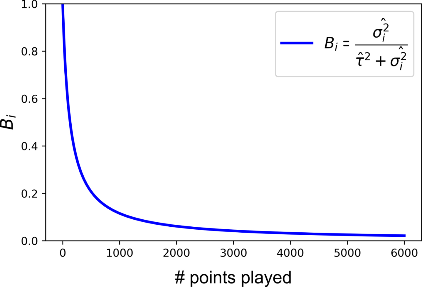
Figure 1 illustrates how normalization coefficient B_i varies with n throughout our dataset. When n is small, as in Elahi’s case, the Efron-Morris estimator strongly shrinks estimates toward the mean. Over the first one thousand points of play, however, B_i sharply declines in strength, approaching zero as match history accumulates further.

4.2Opponent-adjusted ratings

To illustrate the effect of tracking opponent-adjusted statistics, we consider the 2014 US Open first-round match between Mikhail Youzhny (RUS) and Nick Kyrgios (AUS).

From the standard approach, with f_t = .6583, we compute f_ij = .6446, f_ji = .6159. To then calculate opponent-adjusted statistics, we must consider each player’s expected performance given their past opponents. As we observe, Kyrgios has faced slightly stronger opponents than Youzhny over the past twelve months.

In the above table, gi′ represents overall return ability of player i’s opponents in the past twelve months. (1-gi′)*∑nik then represents the expected number of points won on serve given player i’s match history and fi-(1-gi′) the performance relative to this baseline. Opponent-adjusted serve probabilities fij′,fji′ are calculated as follows:

fij′=ft+(fi-(1-gi′))-(gj-(1-fj′))=.6280

fji′=ft+(fj-(1-gj′))-(gi-(1-fi′))=.6413.

Using regular serve parameters, Youzhny is favored to win with π_ij = .6410. With opponent-adjusted serving percentages, we factor in the stronger opponents in Kyrgios’ match history and Youzhny’s win probability drops to π_ij = .4334. As we see, opponent-adjusted ratings can turn around forecasts when one player has faced tougher opponents over the past twelve months.

4.3Klaassen-Magnus elo ratings

Finally, we demonstrate the use of Klaassen-Magnus Elo ratings. In the quarterfinals of the 2016 Olympics at Rio de Janeiro, Kei Nishikori (JP) faced off against Gael Monfils (FRA).

Though Elo ratings clearly favored Nishikori, serve/return statistics over the past twelve months put Monfils at a slight advantage.

f_ij = f_t +(f_i - f_av) -(g_j - g_av) = .6204

f_ji = f_t +(f_j - f_av) -(g_i - g_av) = .6263

To produce serve parameters that reflect Nishikori’s Elo advantage and the pair’s overall serve ability, we implement the approach from Section 3.3 with π_ij = .7094, f_ij = .6204, f_ji = .6263.

fij′,fji′=S(πij,fij+fji)=.6451,.6016

Now we can forecast match outcomes with the hierarchical Markov Model, using serve parameters that respect each player’s Elo rating.

5.1Dataset

This project drew from a publicly available match dataset (Sackmann, 2018). Match summary statistics cover over 150,000 ATP tour-level matches dating back to 1968. Relevant features included:

match date, tournament, surface type, player names

match serve/return statistics

The matches in this repository comprised dataset M , from which we determined players’ historical serve/return performance and Elo ratings. While all methods generated serve parameters from historical data, none required a training set for tuning hyper-parameters. Excluding Davis Cup matches,⁷ we designated all matches from 2014-16 as test set Mt and produced serve parameters for each match in Mt based only on prior matches. Implementations of all methods in this paper may be found at https://github.com/jgollub1/tennis_match_prediction.

5.2Evaluation

All methods produced parameters f_ij, f_ji to estimate each player’s probability of winning a point on serve in a given match. We evaluated methods by predicting both the winner of every match and each player’s percentage of points won on serve. To evaluate serve performance prediction, we considered the RMSE (root-mean-square-error) between each method’s parameters and observed performance. By observing the proportion of points won on serve by each player for a single match k, we obtained s_ik, s_jk and realized error terms e_ik, e_jk: sik=wiknik,sjk=wjknjk

e_ik = |s_ik - f_ij|, e_jk = |s_jk - f_ji| .

Over test set Mt , a method’s RMSE computed to:

r=∑k∈Mteik2+ejk22|Mt|.

To produce match win forecasts, we returned to the hierarchical Markov Model. As a function of a method’s parameters f_ij, f_ji we calculated match win probability π_ij recursively from the probabilities of winning sets and games, as described in Section 2.1. Then we computed accuracy and log loss by comparing these forecasts with observed wins or losses for each match in Mt . In measuring accuracy, we classified π_ij as a predicted win when π_ij ≥ .5 and a loss otherwise.

5.3Discussion

We evaluated methods across 7,622 ATP tour-level matches from 2014-16. To compute Klaassen-Magnus Elo ratings, we set the constraint b = f_ij + f_ji, where f_ij, f_ji were computed with the Efron-Morris Estimator, as described in Section 3.1.1. Because a player’s performance can vary significantly across surfaces, we included a Barnett and Clarke variation which only considers performance on the given match’s surface.⁸ In Table 1 and Table 2, “EM” denotes a variation that used the Efron-Morris estimator to compute f_i, g_i in Barnett and Clarke’s equation.

Table 1 displays each method’s RMSE in predicting the proportion of points won on serve. Of all Barnett-Clarke variations, the surface-based estimator fared worst. This was likely due to decreased sample sizes, as filtering matches by surface limited the amount of available data. Its Efron-Morris variant performed significantly better in all years, suggesting there may be value in a surface-specific approach when bias from limited data is offset. However, this variant only came close to reaching parity with the standard Barnett-Clarke model in the year 2014.

While it was intended to address issues with varying strength of schedule, the Common-Opponent Model underperformed all other methods in predicting serve performance. When two players shared few opponents across their match histories, this approach proved fairly susceptible to bias. Furthermore, while Barnett-Clarke variants considered the past twelve months of data, this approach considered all historical matches, curbing its ability to express recent trends as players’ match histories accumulated. On the other hand, opponent-adjusted ratings demonstrated an improvement to both Barnett-Clarke and the Common-Opponent Model. By estimating serve and return ability on a continuous scale, opponent-adjusted ratings allowed us to consider all matches within the last twelve months and avoid a major shortcoming of the Common-Opponent Model.

Overall, Klaassen-Magnus Elo ratings proved most effective in forecasting serve performance. As Elo ratings were already known to estimate player ability more effectively than point-based models, it follows that adjusting serve parameters in accordance with these ratings would significantly improve forecasts. In contrast, Barnett-Clarke variations still appear to leave out important information by ignoring match outcomes and forecasting strictly from point-level data. While point-based models have often proven necessary for predicting more granular outcomes (Barnett et al., 2006), Klaassen-Magnus Elo ratings reconciled point-based models’ expressivity with Elo ratings’ predictive power. Following the recent work of Kovalchik and Reid (2018), this further demonstrated the effectiveness of synthesizing Elo ratings with point-level models specific to tennis’ scoring system.

When applied to Barnett-Clarke variants, the Efron-Morris estimator improved performance to varying degrees. Presumably, this stemmed from robustness with respect to small sample sizes. To better understand its application to our tour-level match dataset, we consider the distribution of points within player match histories.

Fig.2

Number of points played on serve by players i, j in the past twelve months before every match in Mt .

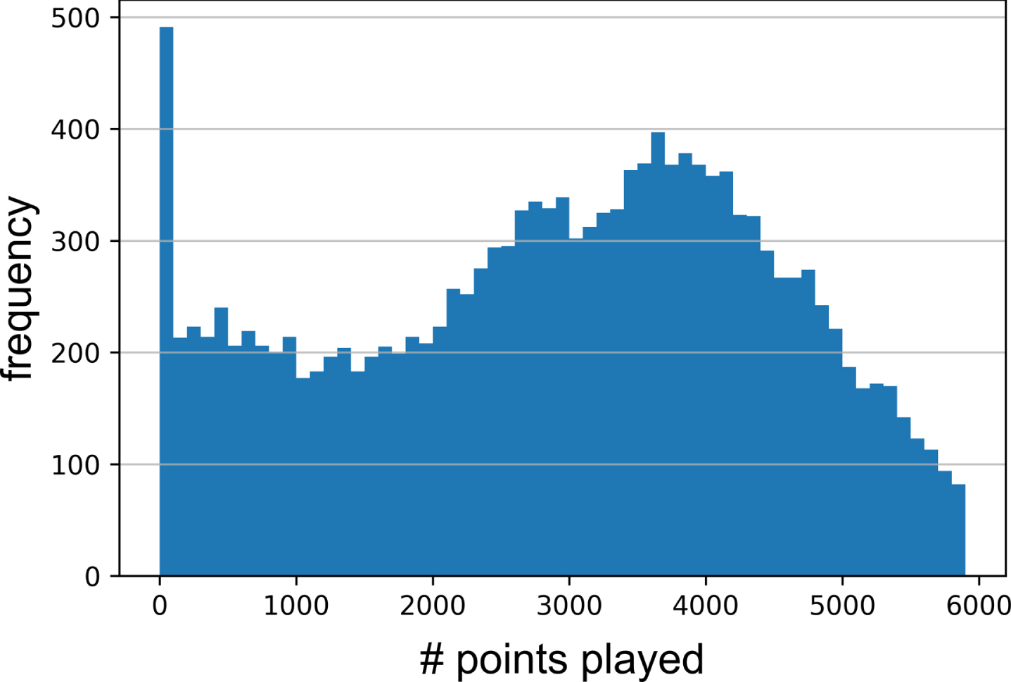
Figure 2 illustrates the distribution of sample sizes when computing f_i, f_j with an Efron-Morris estimator.⁹ Following Barnett and Clarke’s original approach, estimates produced with sample sizes from the leftmost range of the distribution were particularly susceptible to bias. However, recalling normalization strength from Figure 1, we know the Efron-Morris estimator reduced bias by shrinking these estimates furthest toward the mean. Since players accumulate return points over time at approximately the same rate, we can assume the estimator normalized g_i, g_j in a similar manner. If only by reducing errant predictions in this range, the Efron-Morris estimator succeeded in helping all Barnett-Clarke variants more effectively predict serve performance.

Table 2 details each method’s performance in predicting match winners, where many of the same trends surfaced. Once again, variations with an Efron-Morris estimator outperformed their counterparts. In most cases, the improvement in log loss was greater than that of accuracy, supporting the notion that this estimator mitigates extreme results when faced with limited data. The opponent-adjusted model performed several percentage points better than Barnett and Clarke’s original approach across all years, establishing itself as the most effective point-based method surveyed in this exploration. Once again, Klaassen-Magnus Elo ratings predicted outcomes most effectively. However, it is worth noting that its output produced win probabilities identical to those of the Elo ratings fed into the model. In that regard, its relative performance confirmed results from previous studies noting Elo’s dominance in match prediction (Kovalchik, 2016).

References

1 | Barnett, T. and Clarke, S. R. (2005) , Combining player statistics topredict outcomes of tennis matches, IMA Journal of ManagementMathematics 16: (2), 113–120. |
2 | Barnett, T. J. , Clarke, S. R. , et al., (2002) , Using microsoft excel to model a tennis match. In 6th Conference on Mathematics and Computers in Sport, pages 63-68. Queensland, Australia: Bond University. |
3 | Barnett, T. J. , et al., (2006) Mathematical modelling in hierarchical games with specific reference to tennis. PhD thesis, Swinburne University of Technology. |
4 | Bialik, C. , Morris, B. , and Boice, J. (2016) , How we’re forecasting the 2016 u.s. open. http://fivethirtyeight.com/features/how-were-forecasting-the-2016-us-open/. Accessed: 2017-10-30. |
5 | Efron, B. and Morris, C. (1975) , Data analysis using stein’s estimatorand its generalizations, Journal of the American StatisticalAssociation 70: (350), 311–319. |
6 | Efron, B. and Morris, C. N. (1977) , Stein’s paradox in statistics. WH Freeman. |
7 | Elo,A. E. (1978) , The rating of chessplayers, past and present. Arco Pub. |
8 | Klaassen, F. J. and Magnus, J. R. (2003) , Forecasting the winner of atennis match, European Journal of Operational Research 148: (2), 257–267. |
9 | Klaassen, F. J. G. M. and Magnus, J. R. (2001) , Are points in tennisindependent and identically distributed? evidence from a dynamicbinary panel data model, Journal of the American StatisticalAssociation 96: (454), 500–509. |
10 | Knottenbelt, W. J. , Spanias, D. , and Madurska, A. M. (2012) , Acommon-opponent stochastic model for predicting the outcome ofprofessional tennis matches, Computers & Mathematics withApplications 64: (12), 3820–3827. |
11 | Kovalchik, S. and Reid, M. (2018) , A calibration method with dynamic updates for within-match forecasting of wins in tennis, International Journal of Forecasting. |
12 | Kovalchik, S. A. (2016) , Searching for the goat of tennis winprediction, Journal of Quantitative Analysis in Sports 12: (3), 127–138. |
13 | Newton, P. K. and Aslam, K. (2009) , Monte carlo tennis: a stochasticmarkov chain model, Journal of Quantitative Analysis inSports 5: (3). |
14 | Sackmann, J. (2018) , Tennis atp. https://github.com/JeffSackmann/tennis_atp. |
15 | Spanias, D. and Knottenbelt, W. J. (2012) , Predicting the outcomes oftennis matches using a low-level point model, IMA Journal ofManagement Mathematics 24: (3), 311–320. |
Appendices
Appendix A: Common-Opponent Model
Consider a match between players i and j, who share N common opponents throughout their entire match histories. To quantify their relative performance against opponent Ck, let spw(i, Ck) denote the percentage of service points won by player i against opponent Ck and rpw(i, Ck) the corresponding percentage of return points won. We may quantify player i’s advantage over player j with respect to opponent Ck as follows:
Then we approximate match win probability in terms of this relative advantage.
In the above equation, M3(f, g) denotes player i’s win probability in a best-of-three match with f, g representing their probability of winning a point on serve and return, respectively. To compute πij via the Common-Opponent Model, we average the win probability over all N common opponents shared:
While Knottenbelt did not originally use this model to predict serve performance, we inferred parameters fij, fji from the model’s win probability equation as followed:
fij = .6 + Δij/2
fji = .6 - Δij/2 .
Following the above steps, we may predict the winner and serve performance of any match using the Common-Opponent Model.
Notes
1 Knottenbelt’s Common-Opponent model addresses strength of schedule at the cost of reducing the amount of available match data. Kovalchik and Reid’s approach indirectly addresses both of these issues through the use of Elo ratings.
2 The constants in this equation are parameter values that FiveThirtyEight’s team chose after fitting this model on decades of tour-level match data.
3 Tennis’ Open Era began in 1968, when professionals were allowed to enter grand slam tournaments.
4 For current month m, we only collect month-to-date matches.
5 The number of player j’s service points in match k is equal to the number of player i’s return points in match k.
6 For this project, we set ε = .001.
7 Davis cup matches frequently involve lower-ranked players.
8 All matches occurred on hard, clay, or grass courts.
9 For given match k with serve parameters