
The evaluation of pace of play in hockey
Abstract
This paper explores new definitions for pace of play in ice hockey. Using detailed event data from the 2015-2016 regular season of the National Hockey League (NHL), the distance of puck movement with possession is the proposed criterion in determining the pace of a game. Although intuitive, this notion of pace does not correlate positively and strongly with expected and familiar quantities such as goals scored and shots taken.
1Introduction
In possession sports, pace of play is a characteristic that influences the style of a match. Generally speaking, when the pace of a game is high, the game is more fluid and there is more opportunity for scoring.
There are different measurements of pace for different sports. For example, in the National Basketball Association (NBA), pace is typically measured by the average number of possessions per game. For example, in the 2015-2016 regular season, the Sacramento Kings lead the NBA with 102.2 possessions per game which is contrasted with the Utah Jazz who ranked last with 93.3 possessions per game (see www.espn.go.com/nba/hollinger/teamstats). With more possessions, teams typically score and allow more points. For example, the Sacramento Kings ranked 2nd in the 30-team NBA for total points scored in the 2015-2016 NBA season. The Utah Jazz ranked 30th for total points allowed in the 2015-2016 regular season.
In American football, although there is a clear notion of pace of play, there is no commonly reported statistic that directly measures pace. In the National Football League (NFL), the average number of plays per game is recorded for each team (see www.teamrankings.com/nfl/stat/plays-per-game). Although this statistic is related to pace, it is obvious that poor offensive teams who rarely make first downs have fewer plays per game. Therefore, in football, plays per game for a team is confounded with offensive strength and is not a pure measure of pace. Pace in football can be increased for a team by using a “hurry-up offense” which affords more plays in a given period of time provided that the team continues to make first downs. Furthermore, teams that frequently pass the ball (as opposed to run) typically use up less of the clock and have more plays from scrimmage.
In both basketball and football, increasing the number of possesions can be seen as a strategy, particularly when a team is losing. In basketball, intentional fouling stops the clock and provides more opportunities to score and overcome a deficit. In football, ensuring that plays are terminated by going “out of bounds” stops the clock and provides morepossessions.
In soccer and hockey, there are also notions of pace where a “stretched” game is one that goes from end to end, and is thought to be a game which is played at a high pace. However, in both of these sports, there is again no commonly reported measurement for pace of play.
In this paper, we explore various measures for pace of play in hockey that could also be applied to soccer. In hockey, there is a limited body of literature concerning pace. In a recent investigation, Petbugs (2016) considered the percentage of shot attempts taken by a given team in a game (i.e. the Corsi percentage) and used this as a measure of pace. The idea is that teams that are taking most of the shots are playing at a higher pace. As a measure of pace, an immediate difficulty with the Corsi percentage is that the statistic is associated with the quality of the team. If one team is playing much better, they will be in the offensive zone for a greater period of time and will consequently have a higher Corsi percentage. This however, does not mean that they are playing at a high pace. Hohl (2011) provided a brief discussion on possession metrics where Corsi and the related Fenwick statistics are considered as proxy variables for possession.
What makes this paper unusual is that we essentially report a negative result. In the mathematical sciences, negative results are rarely communicated. For example, if an investigator does not establish a theorem, this does not imply that the theorem is not true. It only means that the investigator was unable to prove the result.
In the experimental sciences, the publication of negative results is also not a widespread practice. Sometimes an experimental result is only seen as significant and publishable if a p-value less than 0.05 is attained (Wasserstein and Lazar 2016). However, there has been an increased calling for the publication of negative results. For example, the reputed multidisciplinary journal PLOS ONE now contains a collection of studies that present inconclusive, null findings or demonstrate failed replications of published work (www.ploscollections.org/missingpieces). Without the recognition of negative results, publication biases are introduced, and this affects the validity of meta analyses. In particular, when controversial and important questions of public safety are at stake, it is important to have access to all major studies, either positive or negative. One can think of examples such as the effects due to second hand smoke, the effects of high voltage transmission lines and the effects due to marijuana legislation.
There is another reason why negative results should sometimes be reported. Granqvist (2015) writes, “it causes a huge waste of time and resources, as other scientists considering the same questions may perform the same experiments”. Our investigation may fall under this category. We believe that our measures of pace are intuitive and sensible. With the advent of the availability of detailed NHL event data, we imagine that other researchers may consider similar investigations of pace to what we have attempted. In the context of hockey analytics, Sam Ventura (analytics consultant for the Pittsburgh Penguins) tweeted, “I’ve said this to a large number of colleagues & students recently, so I’m posting it here too: Null results are still interesting results!” (https://twitter.com/stat_sam/status/7171098864301588488848). Ventura then tweets, “Publish all of your results, regardless of how “strong” or “weak” they are. It can only serve to benefit the research community by putting this information out there.”
In Section 2, we describe the initial approach that we use in defining pace. We also describe the data which we use to investigate various pace of play statistics. The proposed statistics are based on big data sources that take the form of event data. Consequently, the statistics could not have been computed prior to the advent of modern rink technology and computing. In Section 3, we calculate the various pace statistics for the 2015/2016 NHL season. We observe that none of the proposed statistics correlate positively with expected and familiar quantities such as goals scored and shots taken. Consequently, there is no appealing narrative for how pace affects games, how pace should be used as a tactic, etc. We conclude with a brief discussion in Section 4.
2Pace calculation
Our understanding of pace is that the pace of play is fast when teams are rushing from end to end, attacking and retreating. In fast paced games, there is less opportunity to be organized in the defensive zone in terms of the numbers of defensive players and positioning. A team that sends players forward exposes themselves to counter-attacks. When a team has the puck and are moving sideways or passing backwards, then they are behaving cautiously and we would say that they are playing at a slow pace. We now attempt to incorporate these general ideas.
Our initial game pace statistic is evaluated as follows: We consider the consecutive events E1, …, En in a game consisting of n events. For each i = 1, …, n, the location of the event Ei is obtained according to the Cartesian coordinates (xi, yi) where (0, 0) is centre ice and (-100, 0) is the position directly behind the home team’s goal. Rink sizes in the NHL are standardized with dimensions of 200 feet by 85 feet. It is important to note that teams change ends at the beginning of the second and third periods.
For each i = 1, …, n, we determine whether the home team (H) or the road team (R) had possession of the puck immediately following Ei. We then determine which team had possession immediately preceding Ei+1. If it is the same team, then there is a pace contribution di which is the “attacking distance” travelled and is defined by
(1)
We therefore define a pace contribution di only in the case of a team moving forward in an attacking direction with possession. For example, “dumping the puck” into the offensive zone with retrieval by the defensive team is not considered as a contribution to game pace. Also, drifting sideways with possession is not considered as a contribution to game pace. The total attacking distance in a game is then defined as
(2)
The remaining detail in the calculation of (2) is the determination of possession as required in (1). Thomas and Ventura (2014) have created an R package nhlscrapr that provides detailed event information and processing for NHL games. The scraper retrieves play-by-play game data from the NHL Real Time Scoring System database and stores the data in convenient files that can be handled by the R programming language. The nhlscrapr package can access NHL matches back to the 2002-2003 regular season. We note that there are 10 types of events Ei provided by nhlscrapr as listed in Table 1.
Table 1
The 10 types of mutually exclusive events that are recorded using nhlscraper. The events are listed in order of their percentage frequency from the 2014-2015 NHL regular season based on 451,919 observed events. There are some unlisted rare events and error codes that comprise the remaining 1%. Note that Line Change corresponds to line changes “on the fly” and not line changes that occur during stoppages. A Missed Shot is a shot that was not a shot on goal
| Event Type | Frequency |
| Line Change | 27.2 % |
| Faceoff | 16.8 % |
| Shot on Goal | 15.1 % |
| Hit/Check | 13.7 % |
| Blocked Shot | 7.9 % |
| Missed Shot | 6.4 % |
| Giveaway | 4.5 % |
| Takeaway | 3.7 % |
| Penalty | 2.2 % |
| Goal | 1.5 % |
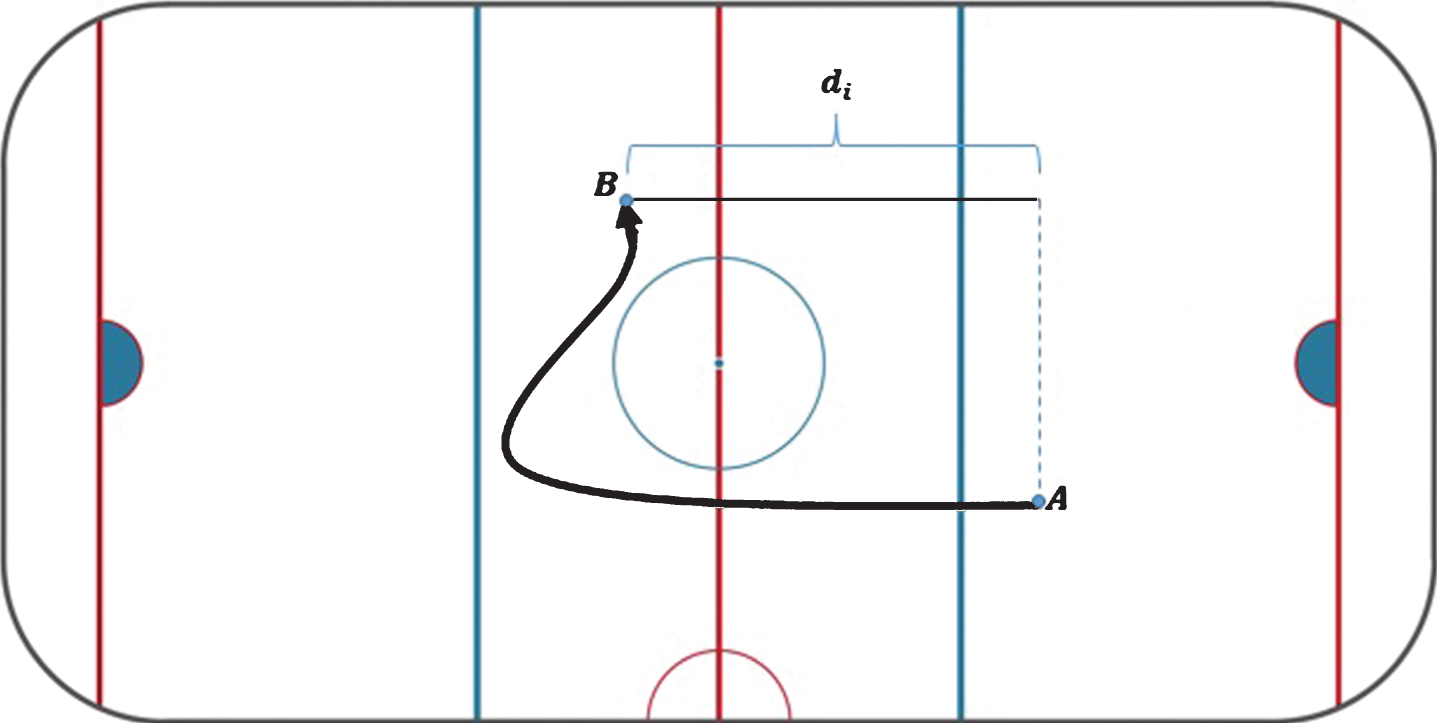
More can be said about the NHL Real Time Scoring System database and the determination of possession. However, a stumbling block with this freely accessible database is that there are roughly 400 events recorded per match. Over a 60 minute hockey game, this translates to an event every 9 seconds on average. Given the action in hockey, much can transpire over 9 seconds, much more than what is recorded in the database. For example, Fig. 1 provides a potential path taken during 9 seconds of possession. In this case, the pace contribution di according to (1) does not reflect the full amount of forward progress made by the team in possession. The skater was moving forward and contributing to pace, but the contribution was reduced by the backward movement. It is even possible for possession to change over a 9 second interval and for this not to be recorded. Consequently, although the NHL Real Time Scoring System database has provided a breakthrough for hockey analytics, it is not detailed enough for our purposes.
Fig.1
Potential path taken by a team during 9 seconds of possession. Given the starting point A and the endpoint B, the pace contribution di is shown.
At this point in time, the NHL is moving towards the collection of data via player tracking cameras in every NHL venue. Consequently, there will soon be an explosion of data in the NHL. A similar initiative has already taken place in the NBA where the SportVU system has been in place since the 2013/2014 season. The NBA data has promoted a surge in research activities including previously difficult topics of investigation such as the evaluation of contributions to defense (Franks et al. 2015). In the NHL, the company SPORTLOGiQ has provided us with proprietary data for most games (1140 out of 1230) during the 2015/2016 NHL season. Most importantly for our purposes, there is great detail in the SPORTLOGiQ database with events occurring every 1.2 seconds on average. Although we are not at liberty to discuss aspects of the SPORTLOGiQ database, we can say that the database has an extended number of events compared to those in Table 1. Furthermore, possession is easily determined so that the calculations of (1) and (2) are easily facilitated. In Section 3, we describe our investigation of pace using the SPORTLOGiQ database.
3Investigation of pace
We begin with the distance metric D defined in (2) which is the sum of forward attacking distances by both teams in a game measured in feet. We have omitted overtime periods because teams may play differently during overtime. Specifically, since the 2015/2016 season, teams play with three skaters instead of five during overtime. This “opens up” the ice and lead to longer periods of possession.
To provide an intuitive measure of pace for a game, we define
(3)
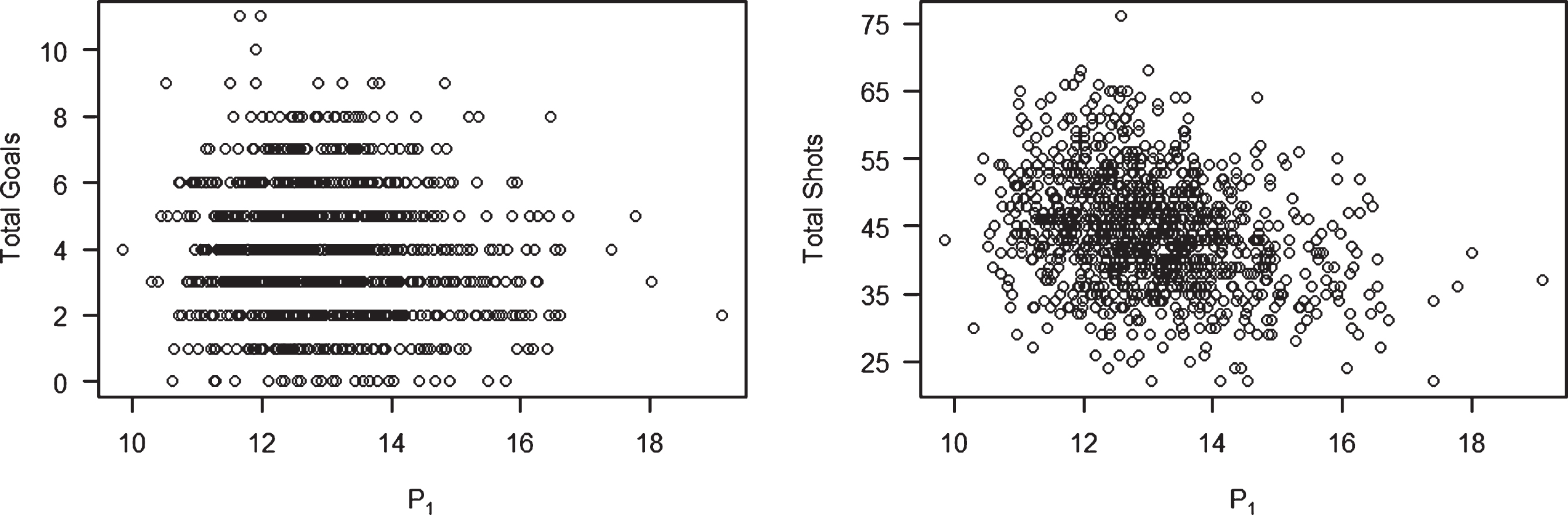
In Fig. 2, we provide scatterplots of the pace variable P1 versus total goals while full strength and versus total shots while full strength in a game. The plots are based on the 1140 recorded SPORTLOGiQ matches during the 2015/2016 regular season. In neither plot do we see a positive correlation. The correlation coefficients for the two plots are -0.079 (total goals) and -0.281 (total shots). This is surprising as one would think that high paced games would lead to more scoring opportunities. In fact, the correlation for total shots r = -0.281 is highly statistically significant (negative) with a t-statistic of
Fig.2
Plots of familiar measures (total goals and total shots while full strength) versus P1 for games during the 2015/2016 NHL regular season.
Since the correlations were surprising, we investigated the definition of pace given by P1 in overtime where the format is 3v3. The median of P1 during overtime (284 games) was 9.94 compared with median value 12.87 during 5v5 play. The comparison suggests that a different style of play (less pacey according to P1) occurs during overtime. Our interpretation is that teams have more “open ice” during overtime where players can skate in various directions and retain possession. This sort of meandering does not contribute to pace as definedby P1.
We further carried out the investigation of P1 by restricting its calculation to first periods involving 5v5 play. There is an intuition that pace may be affected by the score. For example, in a tied game in the third period, teams may play cautiously and at low pace with the hope of entering overtime where at least one match point is guaranteed. By studying the first period only, we suspect that teams may not alter their strategies since it is early in the game. In the first period, the median of P1 was 12.56, not greatly different from the median value 12.87 during all periods. In addition, the correlation of P1 during the first period with total shots in the first period was r = -0.326. This is comparable to the previous surprising correlation r = -0.281 calculated over all periods.
As a second attempt to investigate pace, we modify the calculation of D1 to D2. With D2, we only consider attacking distances di that were traversed at a sufficient speed. The intuition is that teams are not playing at high pace if they are moving slowly. Therefore, we take the attacking distance di in (1) and obtain the time ti in seconds that it took the team to travel the distance di. The time variable ti is available from the SPORTLOGiQ database. Then we only include a di contribution in D2 if di/ti ≥ 5.0 feet per second. This cutoff retains 96.5% of the observations used in calculating P1. This leads to a second measure of pace in a game given by
(4)
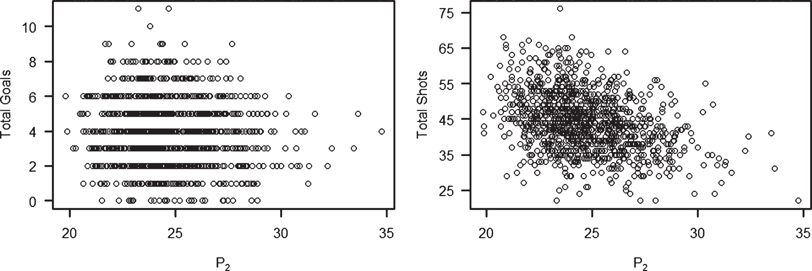
In Fig. 3, we provide scatterplots of the pace variable P2 in (4) versus total goals while full strength and versus total shots while full strength in a game. The plots are based on the 1140 recorded SPORTLOGiQ matches during the 2015/2016 regular season. Again, in neither plot do we see a positive correlation. The correlation coefficients for the two plots are r = -0.091 (total goals) and r = -0.360 (total shots). Here the correlation for total shots is even more negative than with P1.
Fig.3
Plots of familiar measures (total goals and total shots while full strength) versus P2 for games during the 2015/2016 NHL regular season.
We note that we experimented with alternative threshold speeds and observed qualitatively similar results. For example, we increased the threshold from di/ti ≥ 5.0 ft/sec to a much greater di/ti ≥ 20.0 ft/sec. The new cutoff retains 60.4% of the observations used in calculating P1. In this case, the correlation between P2 and shots on goal was r = -0.387 which is similar to r = -0.360 obtained with the lower threshold.
As a third attempt to investigate pace, we modify the calculation of D1 to D3. With D3, we only consider attacking distances di that occurred between the blue lines. The intuition is that frequent transitions between the blue lines (i.e. in the neutral zone) characterize games that have a back-and-forth quality. Operationally, if we have a distance di that begins within a team’s own blue line, we truncate it so it begins at the blue line. If a distance di ends within the opponent’s blue line, then it is truncated to the blue line. This leads to a third measure of pace in a game given by
(5)
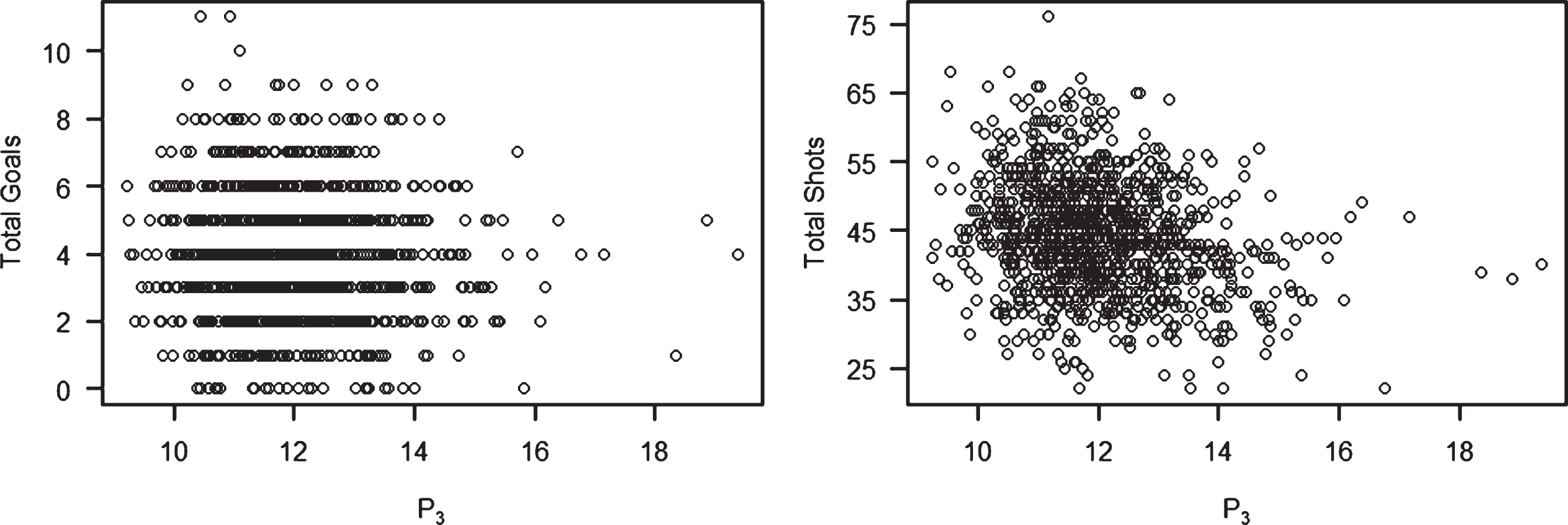
In Fig. 4, we provide scatterplots of the pace variable P3 in (5) versus total goals while full strength and versus total shots while full strength in a game. The plots are based on the 1140 recorded SPORTLOGiQ matches during the 2015/2016 regular season. Again, in neither plot do we see a positive correlation. The correlation coefficients for the two plots are r = -0.040 (total goals) and r = -0.230 (totalshots).
Fig.4
Plots of familiar measures (total goals and total shots while full strength) versus P3 for games during the 2015/2016 NHL regular season.
Finally, it was suggested by one of the referees that we investigate the increasingly popular topic of zone entries. We consider a pace metric P4 based on alternating zone entries. More specifically, when a team first crosses the offensive blue line with possession in a 5v5 situation, we initiate the zone entry counter at Z = 1. When the opposing team next enters its offensive blue line with possession, the counter is incremented according to Z ← Z + 1. We continue to increment Z throughout the game. The idea is that only alternating zone entries are counted so that the notion of back-and-forth play is captured. Similar to before, we define
(6)
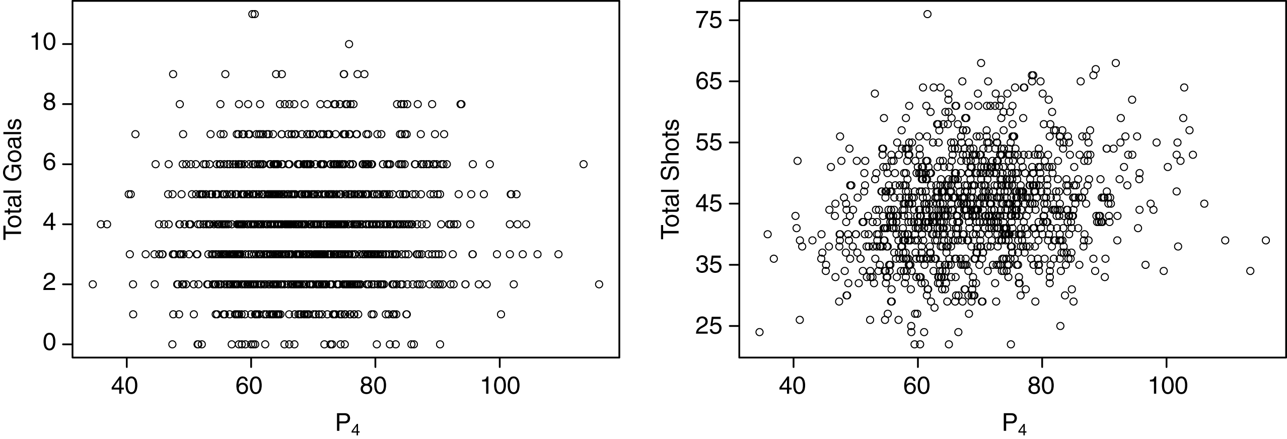
In Fig. 5, we provide scatterplots of the pace variable P4 in (6) versus total goals while full strength and versus total shots while full strength in a game. The plots are based on the 1140 recorded SPORTLOGiQ matches during the 2015/2016 regular season. We observe that the correlation coefficient between total shots and P4 is r = 0.210. This is our only definition of pace (amongst P1, P2, P3, P4) that yields a positive and statistically significant correlation. Whereas the positive correlation conforms to our intuition, the correlation does not strike us as sufficiently large where one might further investigate pacey teams, pacey players, etc.
Fig.5
Plots of familiar measures (total goals and total shots while full strength) versus P4 for games during the 2015/2016 NHL regular season.
4Discussion
This paper introduces various measures for pace of play in hockey which are based on notions of back-and-forth play while in possession of the puck. To our great surprise, we found that our definitions of pace do not correlate positively and strongly with either total goals or total shots on goal. Therefore, our communication may be seen as a negative result. However, since the result is counterintuitive, we believe that it deserves mention in the hockey analytics community.
Should future refinements to the definition of pace provide meaningful positive correlations, then a host of interesting questions may be addressed. For example, does pace contribute to winning? Which teams are pacey? Has pace changed over seasons? Are there pacey players? Can teams incorporate strategies related to pace and goal scoring? At the moment, our pace definition P4 (which is based on the frequency of alternating zone entries) shows the greatest promise as a meaningful measure of pace.
If future research provides a definition of pace where high pace coincides with an increase in goals at both ends of the ice, then a tradeoff between increasing pace and goal scoring may be similar to the tradeoff between pulling the goaltender earlier and goal scoring (Beaudoin and Swartz 2010).
Perhaps one of the takeaways from this investigation is that hockey is not soccer. In soccer, it is well known (Ridder, Cramer and Hopstaken 1994) that scoring intensity increases as a match progresses. As a match wears on, players tire and the game gets stretched. It is during these moments of high pace when goals are more likely to be scored. However, we have seen in hockey that this is not the case. Goals and shots do not increase in games with high pace under the definitions of pace presented here. Rather, one can infer that goals and shots are mostly generated when a team is parked in the offensive zone and the defensive team is under attack.
Acknowledgments
Swartz has been partially supported by grants from the Natural Sciences and Engineering Research Council of Canada. The authors thank two anonymous referees whose comments helped improve the paper.
References
1 | Beaudoin D. and Swartz T.B. (2010) . Strategies for pulling the goalie in hockey, The American Statistician, 64: (3), 197–204. |
2 | Franks A. , Miller A. , Bornn L. and Goldsberry K. . Counterpoints: Advanced defensive metrics for NBA basketball, Sloan Sports Analytics Conference, (2015) . |
3 | Granqvist E. . (2015) . Looking at research from a new angle: Why science needs to publish negative results. In Elsevier Publishing Ethics, Accessed October 4/2016 at, https://www.elsevier.com/editors-update/story/publishing-ethics. |
4 | Hohl G. . Introduction to hockey analytics Part 4.1: Possession metrics (Corsi/Fenwick). In SB Nation: Lighthouse Hockey, www.lighthousehockey.com/2011/8/7/2302188/an-introduction-to-hockey-analytics-part-4-1-an-introduction-to. |
5 | Petbugs. (2016) . Run and gun or slow it down: Identifying optimal game pace strategies based on team strengths. Vancouver Hockey Analytics Conference, Harbour Centre, Simon Fraser University, April 9, recording at, www.stat.sfu.ca/hockey.html. |
6 | Ridder G. , Cramer J.S. and Hopstaken P. . (1994) . Down to ten: Estimating the effect of a red card in soccer, Journal of the American Statistical Association, 89: , 1124–1127. |
7 | Thomas A.C. and Ventura S.L. . (2014) . nhlscrapr: Compiling the NHL Real Time Scoring System Database for easy use in R.R package version 1.8, http://CRAN.R-project.org/package=nhlscrapr. |
8 | Wasserstein R.L. and Lazar N. A. . (2016) . The ASA’s statement on p-values: Context, process and purpose, The American Statistician, 70: (2), 129–133. |


