
Predicting plays in the National Football League
Abstract
This paper aims to develop an interpretable machine learning model to predict plays (pass versus rush) in the National Football League that will be useful for players and coaches in real time. Using data from the 2013–2014 to 2016–2017 NFL regular seasons, which included 1034 games and 130,344 pass/rush plays, we first develop and compare several machine learning models to determine the maximum possible prediction accuracy. The best performing model, a neural network, achieves a prediction accuracy of 75.3%, which is competitive with the state-of-the-art methods applied to other datasets. Then, we search over a family of simple decision tree models to identify one that captures 86% of the prediction accuracy of the neural network yet can be easily memorized and implemented in an actual game. We extend the analysis to building decision tree models tailored for each of the 32 NFL teams, obtaining accuracies ranging from 64.7% to 82.5%. Overall, our decision tree models can be a useful tool for coaches and players to improve their chances of stopping an offensive play.
1Introduction
Football teams are composed of offensive and defensive players. By virtue of having the ball, the offense dictates the play. Because the defense can only react when the opposing team’s offense commences a play, the ability to correctly predict the type of play the offense will run can be a game-changing advantage. At the very least, having clues on the type of play the offense will run allows the defense to make better-informed decisions and increase their likelihood of limiting the advancement of the other team.
The idea of utilizing prediction for in-game situations has become an increasingly popular research focus in sports analytics (Alamar, 2013). However, the primary objective of previous papers in this area has been to maximize prediction accuracy, which often results in accurate but uninterpretable models. Such an approach is useful to test how far prediction models have advanced or how easy different outcomes are to predict, but they typically do not translate into a practical approach for utilizing those predictions in an in-game situation. For example, accurate predictions from a neural network model may not be implementable if the necessary technology to communicate the predictions and turn them into actionable decisions is not allowed on the sidelines. The National Football League (NFL) is an example of a league with such sideline technology restrictions. In addition, the opaqueness of many complex modeling approaches such as neural networks and random forests, combined with the likely skepticism of coaches to trust complex models they do not understand, limits the potential adoption of such models.
In this paper, our goal is to create an interpretable prediction model that can be used by anyone and that is accurate, motivated by the desire to see such models used in real game situations. Our focus is on predicting plays—in particular, whether the play will be a pass or rush –in the NFL. We start by creating several different prediction models to determine which one achieves the highest prediction accuracy; this result serves as a baseline for comparison for our “practical model” as well as validation against published literature using different datasets. After demonstrating that our highest accuracy model is competitive with the state-of-the-art, we investigate a family of simple decision tree models to determine the trade-off between accuracy, false negative rate, and model parsimony. We further investigate the performance of team-specific models, which are trained on only a fraction of the data. The data we use includes 130, 344 NFL regular season plays from the 2013–14 season to the 2016–17 season, inclusive.
Our specific contributions in this paper are as follows:
1. We show that a neural network model generates a maximum prediction accuracy of 75.3% with a 10.6% false negative rate. This prediction accuracy is competitive with the state-of-the-art; false negative rates were not reported for comparable studies.
2. Being the first to view the NFL play prediction problem through the lens of real-world implementation, we devised a simple decision tree model that captures 86% of the accuracy of the complex model.
2Literature review
Recent prediction-based sports analytics research has focused on individual player projections, game outcome predictions, and in-game play-type predictions.
Studies focused on analyzing individual NFL players often attempt to predict their potential and their impact on the field. For instance, Mulholland and Jensen (2014) employed linear regression models and recursive partitioning trees on pre-NFL draft data to predict the career success of tight-ends in the NFL. In another study, Dhar (2011) found that college game statistics and body mass index were significant factors that influenced wide receivers’ success in the league. Alamar and Gould (2008) projected an offensive linemen’s impact on the team’s passing completion rate by using a series of regression trees to determine how likely the lineman was to successfully hold his block in relation to the time it took for the quarterback to throw the ball. Berri and Simmons (2009) investigated the relationship between the draft position of a quarterback and his subsequent performance in the NFL and concluded that the top picks in the real-world NFL drafts are significantly overvalued in a manner that is inconsistent with the notion of rational expectation and efficient markets.
The focus of recent prediction research in other sports, such as basketball and hockey, has been predicting game outcomes. Prediction outcomes of NCAA tournament games (Dutta, Jacobson, and Sauppe, 2017), NBA regular season games (Manners 2016), European hockey league regular season games (Marek, Šedivá, and Ťoupal, 2014), and NHL playoff games (Demers, 2015) have all been examined using a variety of prediction models.
The most similar studies to this paper have also examined the problem of predicting NFL plays, but with the goal of maximizing accuracy. Lee, Chen and Lakshman (2016) used play-by-play data and Madden NFL video game player ratings from the 2011–12 to 2014–15 seasons in a mixed model involving gradient boosting and random forests to achieve a prediction accuracy of 75.9%. Burton and Dickey (2015) used data from the 2011–12 to 2014–15 seasons and built logistic regression models for each quarter and for winning, tied, and losing situations in the 4th quarter, achieving a prediction accuracy of 75.0%.
3Data
3.1Data sources
We obtained our raw data from two sources: (1) play-by-play data from www.NFLsavant.com, (2) Madden NFL video game player ratings from maddenratings.weebly.com.
3.1.1Play-by-play data
We obtained detailed play-by-play data for four NFL regular seasons, from 2013-2014 to 2016-2017, which included 1034 games and 130,344 pass/rush plays in total. For each play, we recorded the year, quarter, minute, second, down, yards to go for first down, yard line, and offensive formation (shotgun, wildcat, under center, and whether there was a huddle or not). It should be noted that intended passing plays that reverted into QB scrambles were still classified as passing plays. The play-by-play data provided most of the raw features that we used to build the prediction models.
3.1.2Madden ratings
We obtained the overall player rating, which is a weighted sum of ratings along several attributes, for each player from the 2014 to 2017 versions of the Madden NFL video game. These ratings are based on player performance from the previous season which allows us to use them to predict plays for the upcoming season. For example, Madden 14 is based on data from the 2012–13 season and we use these ratings to predict plays for the 2013–14 season. The Madden data augmented our play-by-play data with a degree of (subjective) domain knowledge that captures more subtle differences in the strengths of the teams. For example, a team with outstanding wide receivers or an offense facing a team that is adept at defending rushes are both more likely to pass the ball.
3.2Derived features
Using the raw play-by-play data, we derived additional features that give insight into a team’s in-game tendencies. These features included the previous play, whether the game was home or away, point differential, in-game and in-season passing proportion, in game completion proportion for passes and the average yards gained for a pass/rush.
Using the Madden player ratings, we derived scores for eight position groups on each team: quarterback, running backs, wide receivers, offensive line, defensive line, linebackers, cornerbacks and safeties. In order to compute these scores, we took the number of players needed on the field for each position group (based on the I offensive formation and the 4-3 defensive formation) from highest to lowest score rank, and then the scores of the selected players were averaged to compute the position group score. Our reason for selecting the number of players for each position group was to avoid penalizing teams that have low-rated back-up players who rarely see the field.
3.3Exploratory data analysis
In this subsection, we provide a brief overview of insights gained from an initial exploratory analysis of our dataset. Overall, 58.9% of plays were passing plays, which represents the baseline accuracy of a naïve prediction model that predicts pass for every play. Drilling down a little deeper, when the dataset is divided by downs, the proportion of passing plays on 3rd down is approximately 79.3%, which is substantially higher than other down scenarios as shown in Table 1. This result is intuitive as passing plays typically result in more yards gained, which increases the chance of a successful 3rd down conversion for longer distances.
Table 1
The proportion of plays that are passes by down, game scenario and Madden rating for quarterback, wide receiver and running back
| Current down | ||||||
| First | Second | Third | Fourth | |||
| 0.496 | 0.585 | 0.793 | 0.670 | |||
| Game scenario | ||||||
| Losing | Tied | Winning | ||||
| 0.656 | 0.558 | 0.513 | ||||
| Madden rating | ||||||
| [70, 74] | [75, 79] | [80, 84] | [85, 89] | [90, 94] | [95, 99] | |
| QB | 0.591 | 0.576 | 0.587 | 0.583 | 0.594 | 0.612 |
| WR | 0.526 | 0.594 | 0.583 | 0.587 | 0.614 | n/a |
| HB | 0.609 | 0.597 | 0.588 | 0.566 | 0.586 | n/a |
Further shown in Table 1, a team is more likely to pass (65.6%) when behind in the game, compared to when the team is leading (51.3%). This finding is also intuitive because passing plays are seen as higher reward and higher risk: there is the potential to gain more yards, but also an increased chance of a turnover via interception or an incomplete pass.
The Madden ratings of the position groups also indicate differences in passing proportion among NFL teams (Table 1). For instance, teams with higher rated quarterbacks, higher rated wide receivers or lower rated running backs are generally more likely to choose passing plays.
4Models to maximize prediction accuracy
Although our focus in this paper is to develop an interpretable prediction model, we start with training a family of “complex” models with the goal of maximizing prediction accuracy. This exercise serves two purposes. First, we wish to validate that our predictions are competitive with the state-of-the-art complex models from other papers. Second, we can use the accuracy achieved by our best-performing complex model as a baseline for the simpler models we develop.
Using our full dataset of raw and derived features, we considered the following four models: classification trees, k-nearest neighbors, random forests, and neural networks. The respective hyperparameters for each model were tuned using repeated 10-fold cross validation over 15 iterations. Because maximizing prediction accuracy was the goal, prediction accuracy was used as the scoring metric for cross validation. However, we also considered the false positive (i.e., predict pass when it is a run) and false negative (i.e., predict run when it is a pass) rates of each model. Given the practical interpretation of these two metrics, we believe the false negative rate is the more important metric to consider. A defense that is expecting a pass will generally be in a better position to respond to a run, compared to a team that is positioned to defend against a run when a pass play is executed instead.
Table 2 compares the prediction accuracy and false negative rate of the four models. The neural network has the highest prediction accuracy (75.3%) and is associated with the second lowest false negative rate (10.6%). Recall from the literature that the two closest studies to ours generated prediction accuracies of 75.9% and 75.0%, which suggests that our result is competitive with the state-of-the-art. The other papers did not document their false negative rates, so we cannot comment with certainty about how our rate compares. The importance of each feat0ure in prediction accuracy is highlighted the appendix.
Table 2
The prediction accuracies and false negative rates for each of the complex models
| CART | KNN | Random forest | Neural network | |
| Prediction Accuracy | 73.3% | 71.3% | 74.7% | 75.3% |
| False Negative Rate | 11.9% | 6.7% | 11.1% | 10.6% |
5An interpretable prediction model
The design of our simple prediction approach was guided by two criteria. First, the prediction model must be easy to execute in the short time frame that the defensive coordinator has to make a play calling decision. In the NFL, the offense has a maximum of 40 seconds in which they can snap the ball. Within the first 25 seconds, the defensive coordinator can communicate, via a one-way radio, to the middle linebacker. Therefore, to ensure that the model is quick to use, we limited the variables that the simple model could utilize to static variables that can be easily observable at any point in time. By doing so, we eliminated variables such as the in-game passing proportion, or the average yards gained per pass within the game, which would require the coach to constantly update and keep track of throughout the game. The only static variables permitted in the simple model were the quarter, down, minute, yards to go for first down, previous yards gained and the point differential. The second criterion was interpretability. We believe coaches are less likely to trust and adopt a black box model. Thus, the simple model must be understandable by any who uses it. Given these two criteria, we ultimately decided to implement a classification tree model with a limited number of splits.
To determine an acceptable balance between accuracy and simplicity, we trained a large family of classification tree models that differed in how many variables were included and how many splits were allowed. After obtaining the results of each attempted simple model, the next step was to select the optimal one, considering a complexity vs. accuracy trade-off. We thought that having fewer variables, while maximizing prediction accuracy, would be desirable as it would require fewer inputs to keep track of and consider before making a prediction. Thus, we ended up choosing a classification tree with three variables and 10 splits, which generated the highest prediction accuracy among all of the trees considered.
The chosen classification tree is depicted in Fig. 1. The three variables that had the greatest impact on play prediction were the current down, yards to go for first down, and point differential. This simple model achieved a prediction accuracy of 65.3%, which corresponds to 86% of the accuracy generated by our neural network model. Finally, we created an equivalent visual representation of the classification tree that we believe is even easier to read and/or memorize, which may be useful in the time-sensitive situations (see Fig. 2). It should be emphasized that this model does not replace a coach’s knowledge but should be used to support decision making. Since we utilized a classification tree, we can use the proportion of the majority class in each terminal leaf node as a measure of how strong each prediction is, which allows coaches and players to decide how heavily to trust the model in particular situations.
Fig. 1
A classification tree that can be readily used by coaches with the percentage of the majority class in parenthesis.
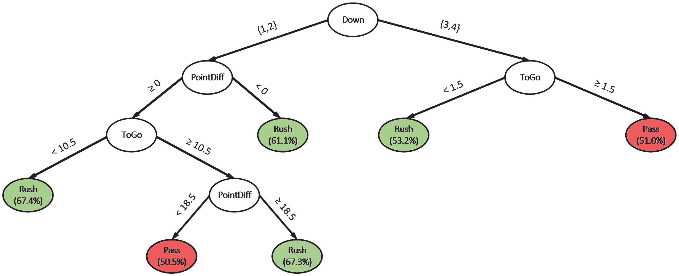
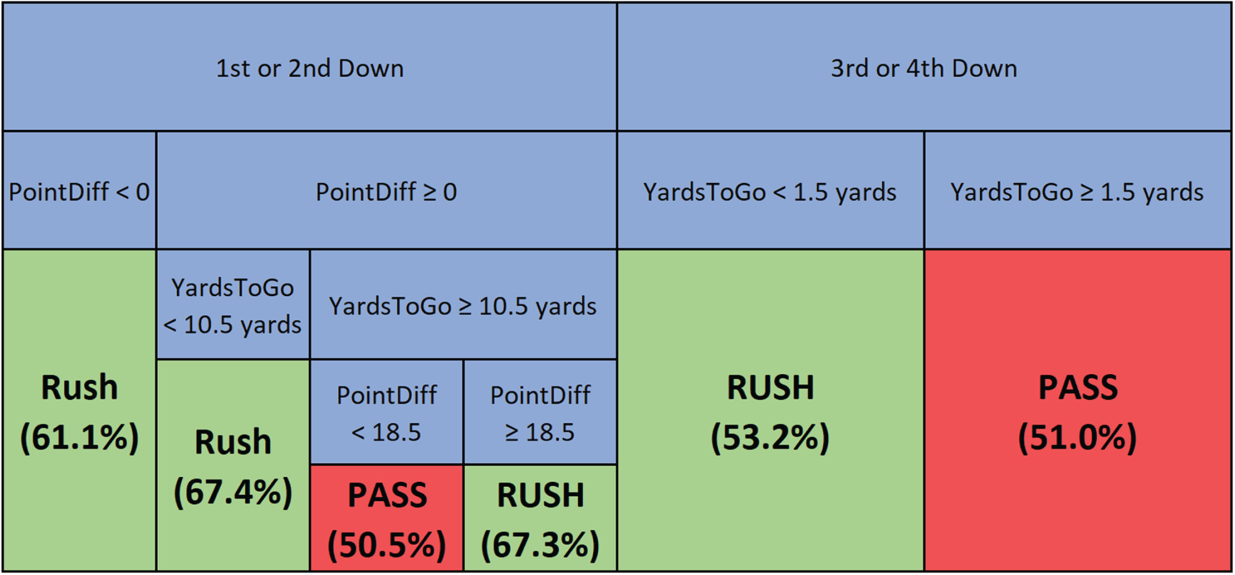
Fig. 2
An equivalent representation of the coach’s classification tree with the percentage of the majority class in parenthesis.
The predictive accuracy of the model based on different games scenarios is shown in Table 3. For example, we find that the model’s prediction accuracy is higher in the fourth quarter, on third and fourth downs, when the offense is losing and when the yards to go is greater than 13. On the other hand, model performance is fairly stable across all yard lines.
Table 3
The prediction accuracies of the classification tree based on different game variables
| Current quarter | ||||
| First | Second | Third | Fourth | |
| 60.3% | 60.6% | 62.4% | 73.1% | |
| Current down | ||||
| First | Second | Third | Fourth | |
| 58.8% | 58.7% | 84.2% | 83.4% | |
| Current yard line | ||||
| 1–24 | 25–49 | 50–74 | 75–99 | |
| 63.7% | 64.2% | 64.9% | 64.3% | |
| Game scenario | ||||
| Losing | Tied | Winning | ||
| 66.6% | 60.6% | 62.9% | ||
| Yards to go | ||||
| 1–4 | 5–8 | 9–12 | 13–16 | 17+ |
| 66.7% | 66.4% | 61.2% | 77.9% | 76.0% |
In addition to providing defensive coordinators with tools to assist play calls, the model also serves as a means of supplying the individual players on the defensive line with “pre-snap reads.” Players can run through the model and determine with greater likelihood whether it will be a pass or a rush, and mentally prepare themselves for the ensuing play. For example, if a safety uses the model and predicts a pass, this can inform him to take extra caution in guarding the wide receivers. The model could be inserted in a play-call wristband similar to the ones used by quarterbacks. Since the players can utilize the model up until the time of the snap, we are able to create a secondary model with the addition of the offensive formation variable (Figs. 3 and 4). This new model achieved a prediction accuracy of 72.3%, which captures 96% of the predictive power of our neural network model. We propose that coaches use our base model to aid play calls while the defensive line uses our secondary model to help make pre-snap reads.
Fig. 3
A classification tree that can be used by the defensive with the percentage of the majority class in parenthesis.
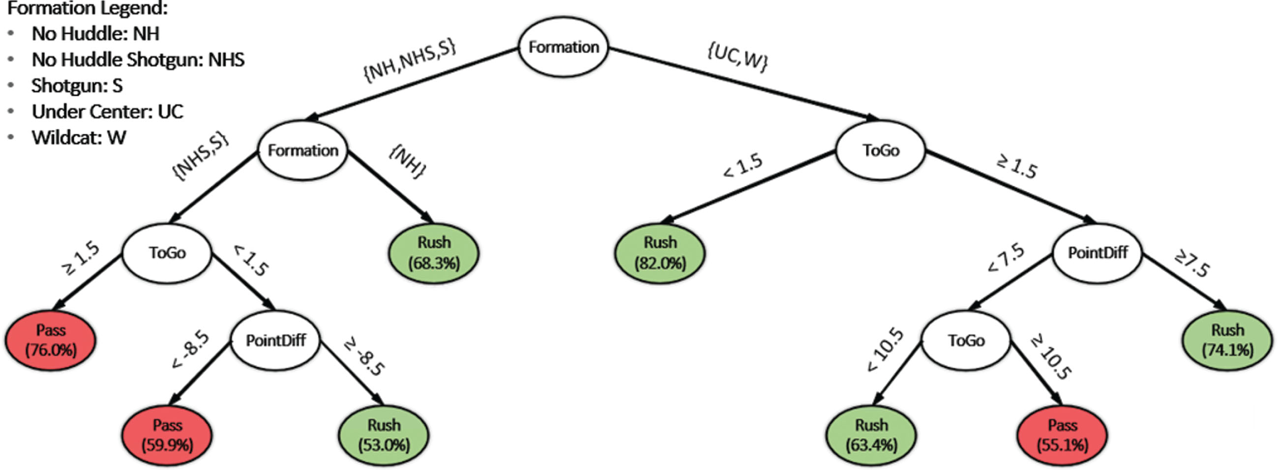
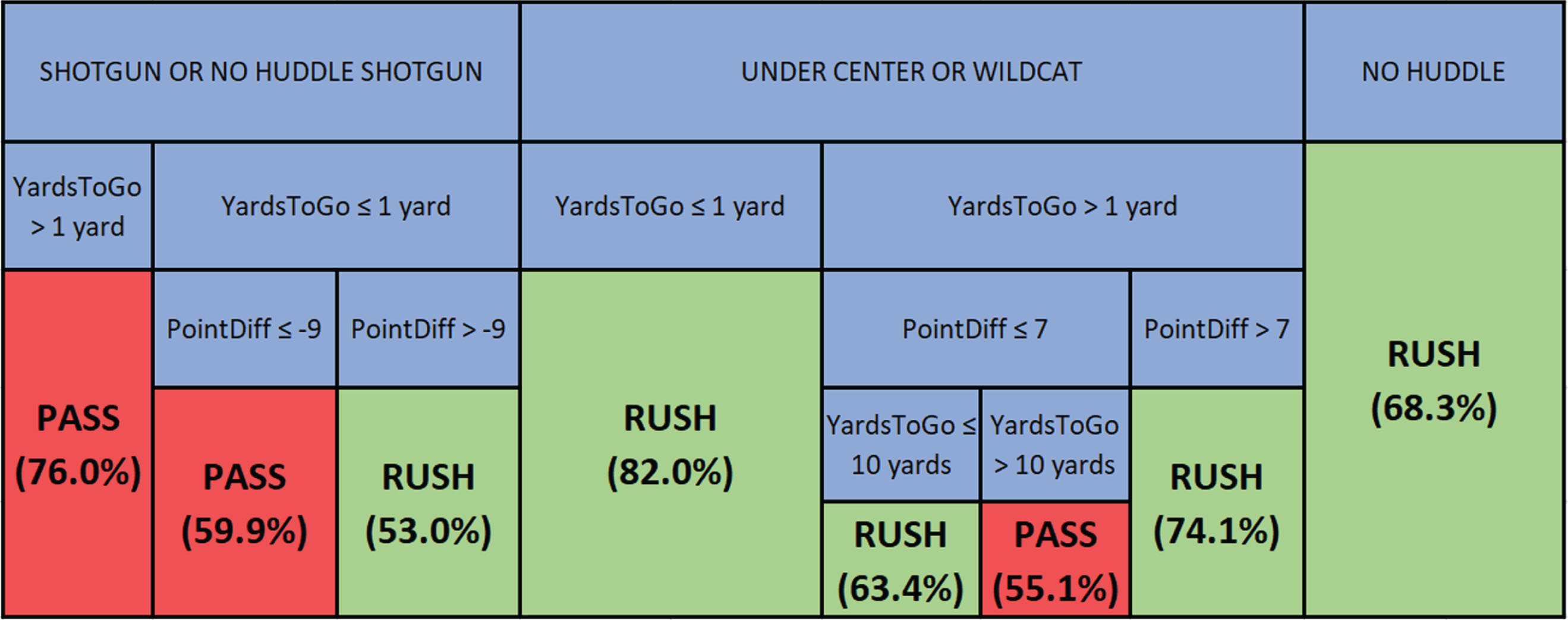
Fig. 4
An equivalent representation of the defensive line’s classification tree with the percentage of the majority class in parenthesis.
6Team-specific classification trees
The previously developed classification trees were trained using data from all teams, and thus is not team-specific. We sought to calculate the predictability of individual teams in order to determine how often teams may deviate from our prediction models described above. Therefore, we created team-specific classification trees following the same approach to balance accuracy with interpretability as previously outlined. Although the process we followed was the same, due to differences in the data for each team, the resulting classification trees differed in the number of variables and splits.
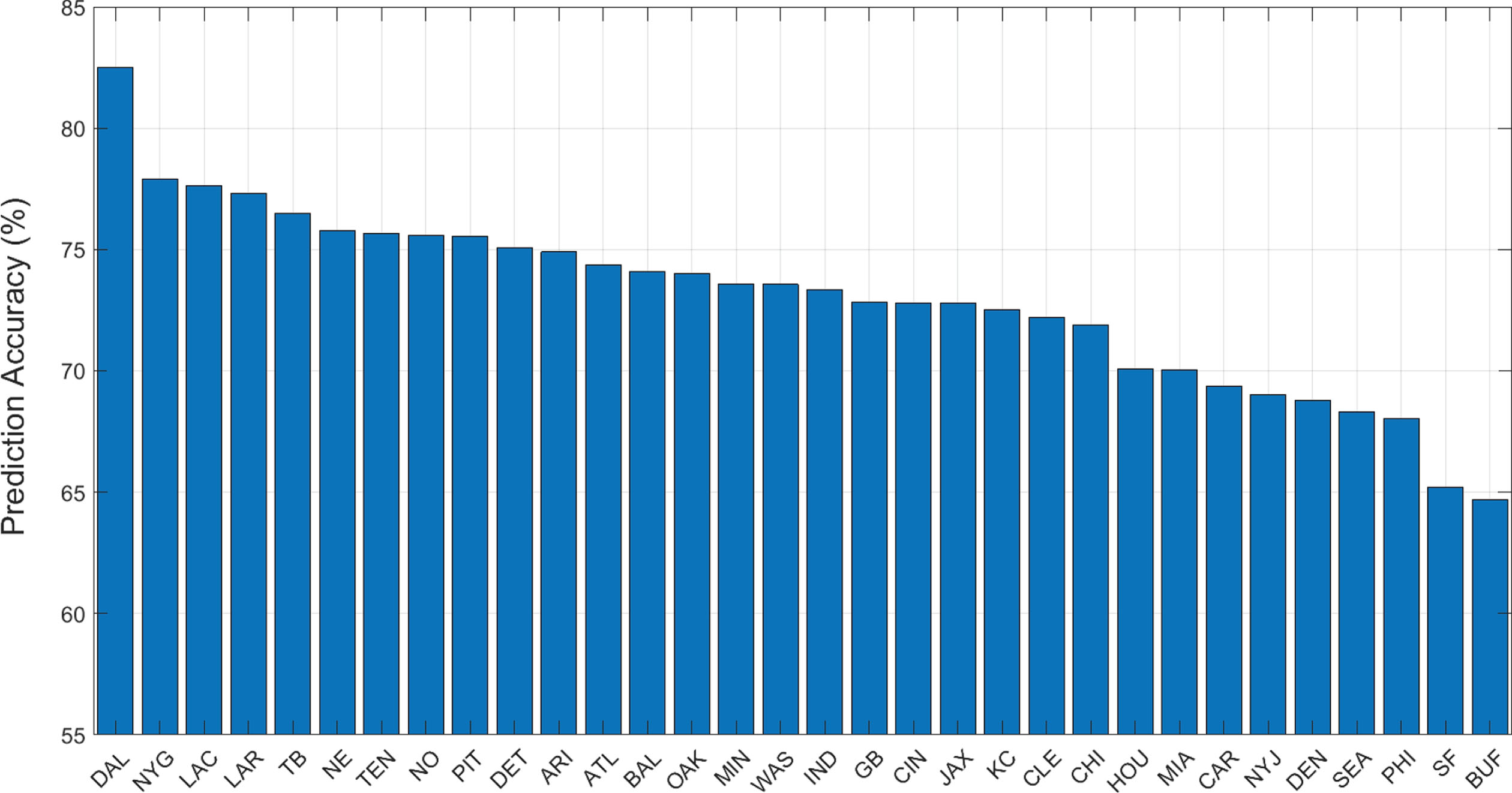
Figure 5 summarizes prediction accuracies of the 32 team-specific models. The model for the Dallas Cowboys achieved the highest accuracy of 82.5%, while the model for the Buffalo Bills achieved the lowest accuracy of 64.7%. The average accuracy over all the team-specific models was 73.0%. We believe the variability in prediction accuracies can be partially attributed to the differences in the offensive styles and tendencies of each team. We found an association between teams with more coaching (head or assistant) changes over the four years spanning our dataset and teams with poorer prediction accuracy. We believe this finding makes sense since as coaches change, styles and play calling tendencies change as well. We also note that teams that are generally always leading (trailing) are easier to predict as they rely more on rushing (passing) plays. However, since the model utilizes point differential as a variable, this feature is already captured by the model.
Fig. 5
Prediction accuracy of the team-specific classification trees.
We further conducted a robustness check to verify that the team-specific results are not due to noise in the data. We randomly assigned each play in the data to a team and re-conducted the analysis, creating 32 new classification trees. We repeated this process 50 times. The average team accuracy was 71.5% (min–max: 70.3% –72.8%), with the average of the minimum values over all teams being 68.9% and the average of the maximum values over all teams being 74.3%. We believe this fairly tight distribution compared to the true distribution with non-simulated data suggests that our original findings were not due to noise and are due to actual between-team variation.
7Future work
There are several avenues of research that we leave for future work. First, more detailed data including the exact players on the field, injuries, weather, even whether players/coaches have made media comments in the days leading up to a game, could lead to better predictions. The addition of this data could lead to the creation of an alternative simple model that avoids using the formation variable but instead uses the exact personnel on the field. This would allow coaches to more readily make play calls based on the model since they do not have to wait until the offensive team gets into formation. Second, related to this first point, testing the model against a human expert would be a valuable exercise, since the human would be able to account for this extra information. Third, it would be of interest to further explore why certain teams are more predictable than others. Perhaps some coaches exhibit fewer variations or more consistency in their play calling. There is also the possibility of training the model sequentially over time as the season progresses to reduce noise associated with player/staff turnover in the offseason. In practice, a hybrid approach where a model trained using historical data and then updated dynamically as the season progresses, may be the most appropriate. Additionally, we note that an even more specific prediction model between a given pair of teams might be valuable to defensive coordinators. That is, the defensive coordinator of the Jets may want not only the Patriots’ team-specific model trained on all Patriots games, but also a Patriots model trained on data from games played exclusively against the Jets. However, as more and more tailoring is desired, the available data to train such a model becomes sparser, possibly leading to reductions in prediction accuracy.
8Conclusion
In summary, this paper focuses on the development of a simple and interpretable machine learning model for predicting NFL plays. We showed that a simple classification tree model with three variables generated an overall prediction accuracy of 65.3%, which is 86% of the accuracy of a state-of-the-art neural network model. Moreover, with the additional goal of creating a simple model that solely aids pre-snaps reads, we were able to achieve an accuracy of 72.3%. When focusing on team-specific data, we are able to show that teams range significantly in terms of predictability, from 64.7% to 82.5%. Given its transparency and the potential to be memorized, we believe our model can be useful as a decision-aid in NFL games, even considering the short timeframe in which these decisions need to be made.
Appendices
Appendix
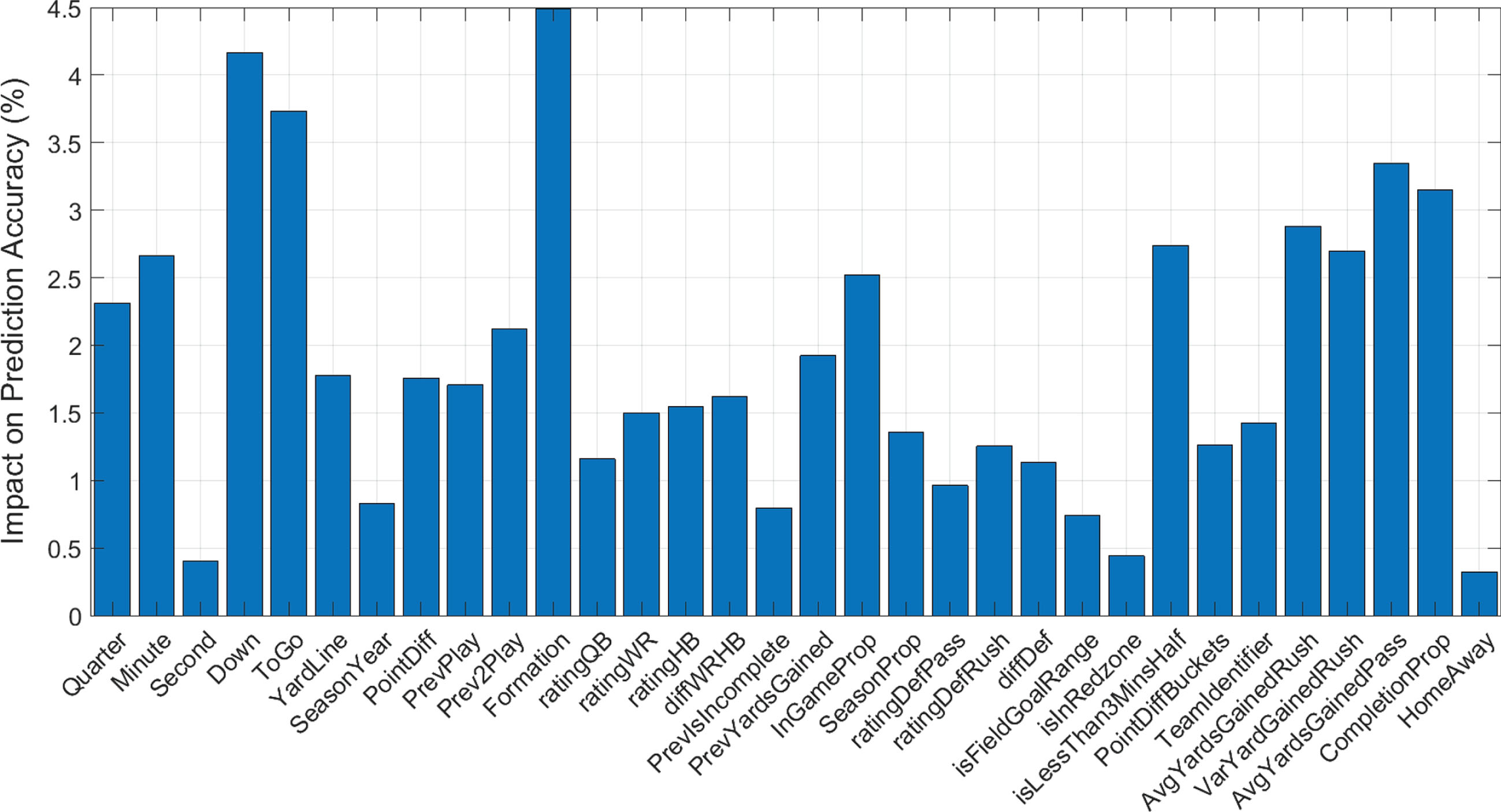
Figure 6 highlights the importance of each feature variable in the random forest model. It is difficult to determine the importance of each feature in a neural network, our best complex model, but we believe that it would be comparable to the results in Fig. 6. It is important to note that the difference in prediction accuracy between the random forest and neural network was only 0.6%.
Fig. 6
The amount of prediction accuracy the random forest model loses if each feature is removed.
References
1 | Alamar B , (2013) , Sports Analytics: A Guide for Coaches, Managers, and Other Decision Makers. New York: Columbia University Press. |
2 | Alamar B & Weinstein-Gould J , (2008) , ‘Isolating the Effect of Individual Linemen on the Passing Game in the National Football League.’ Journal of Quantitative Analysis in Sports, 4: (2), 1–11. DOI: 10.2202/1559-0410.1113. |
3 | Berri D & Simmons R , (2009) , ‘Catching a draft: on the process of selecting quarterbacks in the National Football League amateur draft’ Journal of Productivity Analysis, 35: (1), 37–49. |
4 | Burton W & Dickey M , (2015) , ‘NFL play predictions’ Joint Statistical Meeting 2015. Seattle, 8–13 August. |
5 | Demers S , (2015) , ‘Riding a probabilistic support vector machine to the Stanley Cup.’ Journal of Quantitative Analysis in Sports, 11: (4), 205–218. |
6 | Dhar A , (2011) , ‘Drafting NFL Wide Receivers: Hit or Miss?’ University of California, Berkeley. https://www.stat.berkeley.edu/∼aldous//Old_Projects/Amrit_Dhar.pdf |
7 | Dutta S , Jacobson S & Sauppe J , (2017) , ‘Identifying NCAA tournament upsets usings Balance Optimization Subset Selection.’ Journal of Quantitative Analysis in Sports, 13: (2), 79–83. |
8 | Lee P , Chen R & Lakshman V , (2016) , ‘Predicting Offensive Play Types in the National Football League.’ Stanford University. https://pdfs.semanticscholar.org/37c5/268dc039d4f17bb8cbbe6881bf1bf8187dba.pdf |
9 | Manners H , (2016) , ‘Modelling and forecasting the outcomes of NBA basketball games.’ Journal of Quantitative Analysis in Sports, 12: (1), 31–41. |
10 | Marek P , Šedivá B & Ťoupal T , (2014) , ‘Modeling and prediction of ice hockey match results.’ Journal of Quantitative Analysis in Sports, 10: (3), 357–365. |
11 | Mulholland J & Jensen S , (2014) , ‘Predicting the draft and career success of tight ends in the National Football League.’ Journal of Quantitative Analysis in Sports, 10: (4), 381–396. |


