
Managing In-play Run Chases in Limited Overs Cricket Using Optimized CUSUM Charts
Abstract
In this paper, we present the application of CUSUM control charts to analyze the outcome of a limited overs cricket match during the second innings. This approach makes use of the target set in the first innings and the runs scored from each ball in the second innings. We have analyzed the ball-by-ball data of 1180 One Day Internationals and 537 T20 Internationals played between 2006 and 2017. To improve the accuracy of our models, we have applied genetic algorithm to generate optimal control chart parameters that maximize the accuracy of the model outcome. Our analyses are found to be correct in 80-89% of ODI matches and 76-84% of T20 matches, depending on the stage of in-play analysis.
1Introduction
Cricket, as the age old cliché goes ‘is a game of glorious uncertainties’. While uncertainty is an important part, indeed an essential ingredient, of any sport, the multitude of factors that can influence a game of cricket arguably outnumbers most other games. It is indeed an extremely onerous task to build a model with multiple parameters and then tune those parameters to perfection. Our paper attempts to simplify the task of model building for analyzing the outcome during the second innings of limited overs cricket matches by proposing a mechanism for in-play analysis based only on the runs scored in each ball.
We demonstrate that the target set for the chasing team at the end of first innings and a careful analysis of the ball-by-ball data on runs scored during second innings can help us capture the complexity of a run chase. However, merely deciding on these two parameters is not enough; we need a tool which can capture the uncertainties during the course of a match in a way which can help us achieve our in-play analysis goals. Our paper builds on the concepts of Cumulative Sum (CUSUM) control charts, where chart parameters are optimized using the genetic algorithm to achieve maximum accuracy. CUSUM (Page, 1954) charts take into account both the past and present information and hence, are considered more powerful in detecting small changes in the sample data. Our work is inspired by this property of CUSUM, which helps us in detecting minute changes in run chasing patterns.
We have to define a target for CUSUM charts. Here, we have considered the required runs per remaining ball as the target, and therefore, it is updated continuously. The advantage of making the target dynamic is that the effects of the loss of wickets and overs remaining are automatically incorporated in the target. The reason is that a loss of wicket generally leads to a drop in the runs scored in each ball for the next few overs, which increases the required run rate. Nonetheless, we wanted to determine whether the direct introduction of wickets lost and overs remaining to the model would result in any improvement in accuracy. To incorporate the effects of wickets loss and remaining overs, we considered these two parameters as resources for the batting team and updated the required runs, i.e., target by a factor which was developed using values from Duckworth-Lewis-Stern table (Duckworth and Lewis, 1998; Stern, 2009). However, we did not find any significant difference in accuracy in the outcome analysis for the modified model.
We have worked with a data set of over 1717 limited overs international matches (roughly 0.36 million ball-by-ball data points) during a period of twelve years (2006 to 2017). We have been able to achieve around 80% accuracy level from the halfway mark (25th over) in the second innings of ODIs. We could achieve an accuracy level of around 76% for the same conditions in the case of T20s, which are indeed more difficult to analyze. If we consider the 80% completion stage for the matches (40 overs for ODIs and 16 overs for T20s), our model accuracy is around 87% and 82% respectively. We believe that our paper adds to the literature on in-play forecasting by proposing a simple yet effective framework to analyze the outcome of a cricket match. It also offers a novel approach to the application of control charts to analyze the outcome of a sport. To the best of our knowledge, there is no mention of a similar approach to the problem of in-play analysis in the sports literature.
Rest of the paper is organized as follows. In Section 2, we provide a brief review of the extant literature. In the next section, first, we discuss the data, and then explain the use of CUSUM control charts in analyzing a win or a loss. In Section 4, we apply Genetic Algorithm on our basic models, and then update the models to incorporate effects of overs and wickets in the model. We also discuss the analysis of model accuracy and the choice of the best-fit model in this section. Section 5 concludes the paper.
2Literature review
The body of literature on cricket has witnessed significant advancement in the recent past. Most of the articles concentrate on prescribing the batting order (Swartz et al., 2006; Norman and Clarke, 2010; Preston and Thomas, 2000), player portfolio (Bhattacharjee and Saikia, 2016; Amin and Sharma, 2014), or the effects of various rules on the performance of the teams (Bhattacharjee et al., 2016). There has been a good amount of work on resetting the target for the chasing team in case of interruptions during a limited overs game. One of the pioneering works in this field is Duckworth and Lewis (1998). This work, in some sense also a forecasting model, culminated in the Duckworth-Lewis method which has been adopted by the International Cricket Council for target resetting in all interrupted limited overs matches. Researchers have also worked on modifications to the Duckworth-Lewis method (Stern, 2009; McHale and Asif, 2013), now known as Duckworth-Lewis-Stern (hence, DLS) method. Jayadevan (2004) also developed a method for resetting the target for an interrupted match. ORiley and Ovens (2006) compared both models and concluded that Duckworth-Lewis (D/L) method is better in computing first innings expected score and target resetting, whereas Jayadevan’s method works best only after the completion of first innings.
The literature on forecasting limited overs cricket matches can be traced back to Preston and Thomas (2002) who applied dynamic programming to predict the outcome of a one day international match while it is in progress. Carter and Guthrie (2004) looked at the distribution of runs to be scored at any point in an innings to predict the match outcome. Both the papers are also an attempt to provide an alternative to the DLS method. The work of Morley and Thomas (2005) used logistical regression model to predict the outcome of a match. Bailey and Clarke (2006) developed a forecasting model to predict the margin of victory before the start of the match and then updated the predictions during the match with the help of the Duckworth-Lewis method. Swartz et al. (2009) have studied the outcomes of one day matches by using both modeling and simulation techniques. Singh et al. (2015) also developed models for first innings run prediction and second innings match outcome probability. They applied linear regression and Naïve Bayes classifiers techniques using current run rate and wickets lost for the first innings, and current run rate, wickets lost and target score for the second innings. Recently, Mansell et al. (2018) used running total and total balls bowled to study the difference in runs scored between a winning team and a losing team. They showed the winning team exhibits a better run rate than the losing team as the match progresses. McIvor et al. (2018) used ball-by-ball commentary for predicting in-game events, like boundaries and wickets. They found that more runs are scored in T20 if there are positive comments on batsman and negative comments on bowlers. Patel et al. (2018) developed gradient boosted learning model to predict runs scored in the first innings of T20 and showed that their model outperformed dynamic programming model.
We now focus on the literature specific to forecasting cricket match outcomes. We will discuss the works on unlimited overs (test cricket) matches first before delving deep into the limited overs format. In test match cricket, one of the earliest efforts to predict the match outcome was by Brooks et al. (2002) who used an ordered response model for the task. Scarf and Shi (2005) used a multinomial logistic regression model to aid the team management in deciding the right time to declare an innings. Akhtar and Scarf (2012) developed a multinomial logistic regression model to predict the outcome after each session of play. They could achieve around 80% accuracy level at the end of Day 3. The uncertainties in the test cricket format are different from that of limited overs cricket and as such the above methods cannot be extended to the limited overs format.
Recently there has been a flurry of research work around forecasting the outcome of limited overs cricket matches. For example, Swartz et al. (2009) considered ten different factors for their prediction model. Lemmer (2011) suggested the use of strike rate adjustment to predict batsman’s performance measure in a single match. Norton et al. (2015) used Monte Carlo simulation for in-play forecasting of one day internationals at any stage of the game. They developed a model with six parameters and suggested betting strategies for one day international matches. Kampakis and Thomas (2015) applied machine learning to predict the outcome of English county T20 cricket during 2009-2014. Naïve Bayes produced the highest accuracy, with an average of 62.4%, whereas random forest model had the lowest average accuracy with an average of 55.6%. Asif and McHale (2016) designed a dynamic logistic regression model for in play prediction in one day international matches and demonstrated that the forecast from their model resembles that of the betting markets. The work of Munir et al. (2015) is on T20 games, and the model that they developed achieves 75% accuracy in predicting the winning team. Lemmer et al. (2014) applied a consistency adjusted measure to predict the outcome of a T20 series. For their first model, the success rate is 76.4%, and for the second model, the rate is 70.9%. Mustafa et al. (2017) used social network data and applied machine learning techniques to achieve around 75% accuracy in predicting the outcomes. The body of work discussed above has, in most cases, segregated one day internationals and T20 matches as it is indeed difficult to use the same model to predict these two formats. In papers, where the same model has been used to achieve a reasonable degree of accuracy, the model itself has acquired a complex form. Our work is an attempt to achieve reasonably high accuracy for both the formats of the game and at the same time without compromising the simplicity of the framework.
There has been some work on the application of control charts in the area of sports. Bracewell et al. (2009) applied parametric Shewhart control chart for monitoring individual batting performance in cricket. Cox Dunn 7 and Ryan (2002) used CUSUM chart for analyzing decathlon data to see whether a particular event is resulting in any undue benefit for the more successful athletes. Bracewell (2003) studied the performance of individual rugby players by using control charts.
Genetic algorithm (refer Back et al. (1997) for the literature review on GA) has been used to optimally design CUSUM control charts. However, application of genetic algorithm in the field of sports is mainly limited to team selection in cricket (Omkar and Verma, 2003; Ahmed et al., 2013) and results prediction in football (Rotshtein et al., 2005; Tsakonas et al., 2002).
3Data and methodology
3.1Collection and structuring of data
Our data set (downloaded from the website, http://cricsheet.org/) comprises a total of 1180 ODI, and 537 T20 matches played between 2006 and 2017. There are 604 wins and 576 losses for the chasing teams in ODIs, and 264 wins and 273 losses for the chasing teams in T20s. We have excluded matches that were either abandoned or tied or affected by rain and other reasons where DLS method was used to modify the target. Around 40% of the matches have been randomly selected and used to identify the optimal CUSUM model parameter values and the rest to predict and validate the models. Details about the data set are presented in Table 1.
Table 1
Match break up for GA modeling and Prediction
| ODI | T20 | |||
| Matches | Balls | Matches | Balls | |
| GA modeling | 481 | 124293 | 223 | 24832 |
| Prediction | 699 | 181747 | 314 | 35683 |
| Matches Excluded | 199 | 39 | ||
From the table, we calculated the current and required run rates for the second innings in terms of the average runs per ball. The calculation for other parameters of the control charts in the context of cricket match is discussed in the following subsections.
3.2CUSUM chart for analyzing outcome in cricket
A cricket match can be considered to be evenly poised as long as the control chart values based on the gap between the current run rate and target run rate are within control limits. An upward shift in the value above the upper limit indicates an increase in the chances of winning for the chasing team, whereas a downward shift below the lower limit indicates the opposite. Our dataset shows that for most of the cases, the shift from the target is much smaller compared to the standard deviation of runs per ball. As Shewhart
The CUSUM chart plots cumulative sums of deviations of the sample values from a target value, i.e., CUSUM chart is created by plotting CUSUM values from the first sample set to ith sample set, denoted by
In each one sided CUSUM, we need to consider a decision interval and a reference value. This decision interval is used to calculate the upper and lower control limits based on the standard deviation of the sample. The reference value specifies the size of the shift we need to detect. In control chart theory, both these values are carefully determined to increase the effectiveness in identifying out of control samples.
We will now present the formulation of CUSUM chart in the context of cricket. The notations for parameters and decision variables are given below. Unless otherwise specified, all data related to over i is for the team batting second.
List of notations:
K = Maximum possible number of overs in both the innings (K = 50 for ODI and K = 20 for T20 matches)
M = Total number of overs played in the second innings
Z = Total number of overs considered for analysis
B = Total number of overs data used for analysis = Minimum (Z, M)
In other words, if the total number of overs played in the second innings is less than the number of overs considered for analysis, we only used the limited data points available for analysis.
ni = Number of balls played in over i
xij = Runs scored in the jth ball of ith over
T = Target runs for the second innings to be scored per ball
=
Ri = Required target in runs per ball at the end of over i =
di = ∑i (ni - 1) degrees of freedom for Sp till the end of over i
C4 (di + 1) = An unbiasing constant =
Spi = Pooled standard deviation till the end of over i =
σi = standard deviation of runs till the end of over i =
hu = number of standard deviations between the central line and the upper control limit
hl = number of standard deviations between the central line and the lower control limit
ku = allowable slack in the upward side of the process
kl = allowable slack in the downward side of the process
Note, hu and hl are known as decision intervals. ku and kl are known as reference values.
Then, the value of an upper one-sided CUSUM in over i
(1)
Similarly, the value of a lower one-sided CUSUM in over i
(2)
Consider, LC0 = UC0 = 0
Eqs. 1 and 2 need some explanation in the context of its application in cricket. Note,
Additionally, we also need to define the limits that would confirm whether the gap (i.e., the CUSUM value at either side) in any particular over is significant or not. Hence, we need to compare those high and low CUSUM values with the control limits. To perform the comparison, below we define the upper and lower control limits.
(3)
(4)
The mean, the standard deviation, and the required targets are updated at the end of each over. The values of Ri, LCi, UCi, LCLCUi, and UCLCUi change at the end of each over as
The CUSUM charts in our work have three significant points of departures from traditional CUSUM charts. First, we are interested in separately counting points outside upper and lower control limits after the shifts take place. Hence, our objective is to minimize total errors as opposed to the minimization of Type II errors. Second, due to continuous update in target and standard deviation of runs scored, our CUSUM values and decision intervals are updated with new samples, which makes it dynamic in nature. Finally, our charts are created considering runs scored in each ball played in an over, including no-balls and wide-balls, and thus, we had to modify the models to accommodate unequal sample sizes.
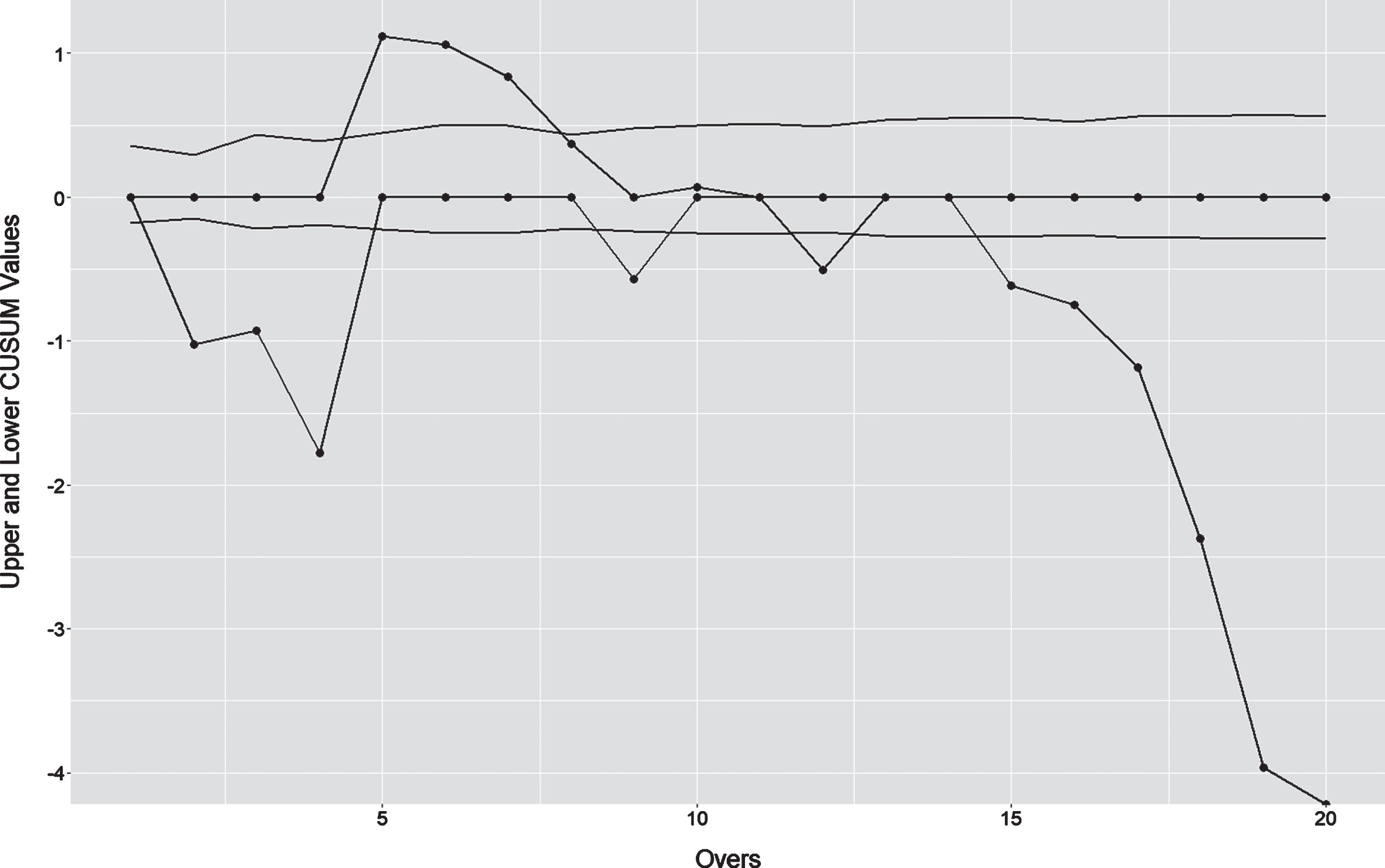
Figure 1 shows an example of CUSUM chart based on the values calculated from ball-by-ball data in the second innings using Eqs. 1 to 4. The match we have considered here is an unsuccessful chase in T20 between South Africa and West Indies (batting second), 2009. In the figure, the dotted lines represent upper CUSUM (UCi) and lower CUSUM (LCi) values, whereas the smoothed lines represent upper control limit (UCLCUi) and lower control limit (LCLCUi).
Fig.1
An Example of CUSUM charts.
For a positive upper CUSUM, if
(5)
(6)
CUi = 1 can be interpreted as a situation when the chasing team’s score shows a significant upward shift in upper CUSUM value. In other words, when CUi = 1 at the end of over i, i.e., the upper CUSUM value is above a predefined higher limit, the cumulative average score till that particular over is significantly above the requirement for the chasing team. This implies an increase in the probability of winning for the chasing team. Similarly, CLi = 1 can be interpreted as a situation when chasing team’s score shows a significant downward shift in lower CUSUM value. In other words, when CLi = 1 at the end of over i, i.e., the lower CUSUM value is below a predefined lower limit, the cumulative average score till that particular over is significantly below the requirement for the chasing team. This indicates a reduction in the probability of winning for the chasing team. Based on the above interpretation, we now propose that if the number of such upward shifts is higher than the number of downward shifts, then the chase would be successful and vice-versa. In mathematical form,
Match Prediction (h, k, ball-by-ball runs) =
(7)
If we consider the CUSUM chart shown in Figure 1, at the end of 10 overs we can see that
4Computational analysis using genetic algorithm
4.1Methodology for basic model
We have designed two types of CUSUM model, basic and modified (to capture other variables, viz., overs left and wickets left). As the performance of CUSUM chart depends on the parameters hl, hu, kl, and ku, there is a need to identify optimal levels of these parameters with a subset of the data available. In terms of prediction, percentage accuracy among a group of matches is considered as the performance indicator. As discussed earlier, around 40% of the matches are considered as a subset for identifying optimal levels of parameters (Table 1).
If a group of L matches is used for measuring percentage accuracy, then the subgroup presentation of these matches can be found in Table 2.
Table 2
Division of matches for comparison between predicted and actual results
| Actual Result | ||
| WIN | LOSS | |
| Predicted Result | ||
| WIN | P | Q |
| LOSS | W | X |
| No Prediction | Z | |
Now, L = P + Q + W + X + Z, where the total number of matched wins and losses = P + X.
(8)
(9)
Also note, P is the accuracy of WIN prediction, and X is the accuracy of LOSS prediction.
We applied the “GA" package (Scrucca et al., 2013) in R to find the optimal values of hl, hu, kl, and ku. We considered OPA as the fitness function and maximized it. For solving each problem, we selected 50 subproblems. For CUSUM, hl, hu, kl, and ku were kept in the open interval of (0, 2). The stop criterion for GA was 50 iterations without improvement. Most of the cases generated multiple optimal solutions. The GA model was run at five different stages of the second innings based on the number of overs left (for ODIs, 25, 20, 15, 10 and 5, and for T20s 10, 8, 6, 4 and 2). Optimal CUSUM chart parameters are shown in Table 3. The accuracy of prediction at different points of the second innings for the methods are shown in Table 4.
Table 3
Optimal CUSUM chart parameters for basic model
| Overs remaining | hl | hu | kl | ku |
| ODI model parameters | ||||
| 25 | 0.8202 | 0.4791 | 0.6255 | 0.4034 |
| 20 | 1.3143 | 0.6842 | 0.5702 | 0.3413 |
| 15 | 0.9193 | 0.8211 | 0.8299 | 0.4341 |
| 10 | 1.0896 | 0.3302 | 0.9932 | 0.7943 |
| 05 | 1.0294 | 0.9921 | 1.0557 | 0.5824 |
| T20 model parameters | ||||
| 10 | 0.7576 | 0.5073 | 0.4921 | 0.3720 |
| 08 | 0.3915 | 0.4380 | 1.0012 | 0.3038 |
| 06 | 0.9790 | 0.4967 | 0.8096 | 0.5410 |
| 04 | 0.3870 | 0.5781 | 1.0720 | 0.4881 |
| 02 | 0.5747 | 0.2496 | 0.9569 | 0.5434 |
Table 4
Percentage accuracy in terms of OPA and PAPM for prediction matches based on optimal chart parameters (Win and Loss predications are also shown separately)
| Match type | Accuracy type | Overs Remaining | ||||
| 25 | 20 | 15 | 10 | 05 | ||
| ODI | OPA | 78.68 | 81.40 | 83.69 | 85.26 | 87.12 |
| ODI | PAPM | 79.71 | 83.19 | 85.28 | 86.50 | 88.91 |
| ODI | Win | 82.90 | 85.49 | 86.4 | 84.47 | 87.29 |
| ODI | Loss | 77.11 | 81.20 | 84.14 | 88.82 | 90.63 |
| 10 | 08 | 06 | 04 | 02 | ||
| T20 | OPA | 71.34 | 75.16 | 76.11 | 78.03 | 82.80 |
| T20 | PAPM | 75.93 | 78.93 | 80.20 | 81.94 | 84.14 |
| T20 | Win | 81.06 | 77.02 | 79.62 | 85.42 | 84.28 |
| T20 | Loss | 71.78 | 81.16 | 80.85 | 78.71 | 84.00 |
Overall percentage accuracy (OPA). Percentage accuracy of predicted matches (PAPM).
To see whether our model is biased towards accuracy in win prediction or loss prediction, we have also captured those results. Our results show that in the case of ODI, as the number of overs remaining increases, win accuracy becomes higher than loss accuracy, and as the number of overs remaining decreases, loss accuracy becomes higher compared to win accuracy. However, both types of accuracy increase with the decrease in number of overs remaining. The justification is as follows. In a match where chasing team has lost most of its batting resources at the start or towards the middle of the innings, the chasing team is likely to lose the match. Though, in general, the effect of wicket loss is immediately reflected in run chasing average, a resultant move from positive UCi value to negative LCi value may take a few overs. As a result, if the analysis is done till the middle of the innings, CUSUM chart may not always be able to predict the loss. The accuracy of the outcome in such cases increases with additional data points. Consequently, at a later stage, UCi reduces, LCi increases, and thus loss accuracy increases. However, in a similar situation, if the chasing team accelerates the run rate only towards the end of innings and wins the match, CUSUM chart may not be able to show a substantial increase in UCi and thus may not be able to predict such a win. This explains the pattern of ODI match accuracy percentages. However, in the case of T20 matches, we did not observe any substantial improvement in loss accuracy towards the end. The intuitive justification is that in case of T20 match, the resource in terms of overs remaining is comparatively fewer. Hence, unlike ODI the chance of not utilizing the remaining overs does not deviate much with the fall of wickets towards the end of the innings. So, the average score per over may not change substantially, and UCi values may not reduce during that phase. Even in case of loss due to early fall of wickets, the same is not reflected in the T20 CUSUM chart at a later stage. Hence, loss accuracy increases for T20, when analyzed from 10 to 12 to 14 overs, but do not show any pattern for othercases.
4.2Models modified using remaining overs and wickets
In this section, we consider additional models where the target of the control chart is modified to capture the effect of the number of wickets lost in the last few overs. In these modified models, both the control limit equations for CUSUM chart (Eqs. 3 and 4) remain unchanged.
One may argue that in a limited over cricket match, a fall of wicket generally results in a drop in the run rate for the next few overs leading to an increase in the required run rate. Fall of a wicket is interpreted as a loss of resource (Duckworth and Lewis, 1998), and is a setback for the chasing team. The intensity of the setback depends on the stage of the match (the number of overs bowled) and the number of wickets lost in the last few overs. This implies that the target becomes harder for the chasing team if they lose a wicket early; for example, losing a wicket in the 15th over makes it tougher compared to losing one in the 30th over. Also, at the 15th over stage, losing three wickets in the previous (14th) over makes the chase tougher as compared to losing only one in the 14th over.
To investigate this additional level of perceived difficulty due to fall of wicket(s), we modify the required run rate with an additional factor, Δ, where Δ is a function of overs played and number of wickets lost in the last few overs. To incorporate the effect of wickets lost, we use standard DLS Tables as a proxy. For ODI, DLS resource table standard edition is taken from International Cricket Council website (https://www.icc-cricket.com/). For T20, DLS resource table standard edition is taken from Bhattacharya et al. (2011).
Our experiments are based on two different procedures to count the number of wickets, a) total number of wickets lost till the end of over i and b) number of wickets lost only within the last ’θ’ overs. We take θ from 0 to 5 overs for ODIs and from 0 to 2 for T20s.
We introduce the following additional notations:
θ = Number of previous overs in consideration
Note, θ = 0 means only effect of overs is considered
Wi = Number of wickets lost in over i
WCi = Combined number of wickets lost till the end of over i =
PRi = Adjusted required run rate
Then,
(10)
Prediction results for models capturing the effect of wickets are given in Table 5. Here we argue that the capability of the batters and opponent team bowlers are automatically ‘captured’ in the run chase behavior. For example, batsman remains cautious at the start of his batting to familiarize with the condition (Lemmer, 2011). In a cricket team, all the players may not have same batting capability, where batting capability is defined in terms of runs scored and overs played. If the number of remaining wickets of the chasing team is considered as an available resource, the batting capability of the resource generally reduces with the reduction in the number of remaining wickets. For example, the average capability of each batsman is higher with ten wickets remaining vis-
Table 5
Percentage accuracy in terms of OPA and PAPM for comparable models (both win and loss accuracy combined) based on optimal GA parameters
| OPA | PAPM | ||||||||||
| ODI | Overs remaining | ODI | Overs remaining | ||||||||
| Models | 25 | 20 | 15 | 10 | 5 | Models | 25 | 20 | 15 | 10 | 05 |
| Basic | 78.68 | 81.40 | 83.69 | 85.26 | 87.12 | Basic | 79.71 | 83.19 | 85.28 | 86.50 | 88.91 |
| Overs | 78.25 | 80.83 | 84.41 | 86.41 | 86.84 | Overs | 79.97 | 82.36 | 85.63 | 87.92 | 88.87 |
| θ = 1 | 78.25 | 81.55 | 84.55 | 85.69 | 87.27 | θ = 1 | 79.85 | 82.73 | 85.65 | 86.94 | 88.66 |
| θ = 2 | 78.68 | 80.97 | 83.98 | 85.41 | 87.55 | θ = 2 | 80.88 | 82.15 | 85.57 | 87.28 | 88.70 |
| θ = 3 | 78.40 | 80.83 | 81.69 | 85.55 | 87.12 | θ = 3 | 80.12 | 82.72 | 83.11 | 87.68 | 88.78 |
| θ = 4 | 78.11 | 80.83 | 83.98 | 86.12 | 87.98 | θ = 4 | 79.71 | 82.60 | 85.44 | 87.12 | 89.26 |
| θ = 5 | 78.25 | 81.12 | 84.98 | 85.26 | 88.13 | θ = 5 | 80.09 | 82.89 | 85.34 | 87.52 | 89.02 |
| Wicket | 78.40 | 81.26 | 84.12 | 84.55 | 86.41 | Wicket | 79.88 | 82.92 | 85.34 | 87.17 | 88.43 |
| T20 | Overs remaining | T20 | Overs remaining | ||||||||
| Models | 10 | 08 | 06 | 04 | 02 | Models | 10 | 08 | 06 | 04 | 02 |
| Basic | 71.34 | 75.16 | 76.11 | 78.03 | 82.80 | Basic | 75.93 | 78.93 | 80.20 | 81.94 | 84.14 |
| Overs | 70.70 | 74.52 | 76.11 | 78.34 | 80.57 | Overs | 76.29 | 80.14 | 79.93 | 81.19 | 84.90 |
| θ = 1 | 70.38 | 74.52 | 75.48 | 78.03 | 81.85 | θ = 1 | 76.21 | 79.32 | 79.26 | 81.40 | 83.99 |
| θ = 2 | 72.29 | 74.84 | 75.16 | 78.66 | 81.53 | θ = 2 | 77.21 | 79.66 | 78.93 | 80.98 | 84.77 |
| Wicket | 71.97 | 73.89 | 75.48 | 78.34 | 81.53 | Wicket | 77.13 | 79.18 | 80.07 | 81.46 | 84.21 |
Overall percentage accuracy (OPA) Percentage accuracy of predicted matches (PAPM)
We also present the accuracy of win and loss for additional models separately in Table 6. The trends of win and loss accuracy percentages show similar behavior as our basic model. The justification for such behavior is already discussed in the previous section.
Table 6
Percentage accuracy in terms of win and loss prediction separately based on optimal chart parameters
| Win Prediction Accuracy | Loss Prediction Accuracy | ||||||||||
| ODI | Overs remaining | ODI | Overs remaining | ||||||||
| Models | 25 | 20 | 15 | 10 | 5 | Models | 25 | 20 | 15 | 10 | 05 |
| Basic | 82.90 | 85.49 | 86.49 | 84.47 | 87.29 | Basic | 77.11 | 81.20 | 84.14 | 88.82 | 90.63 |
| Overs | 83.72 | 83.14 | 85.23 | 86.83 | 86.91 | Overs | 77.02 | 81.61 | 86.05 | 89.09 | 91.05 |
| θ = 1 | 86.43 | 84.69 | 85.59 | 84.47 | 87.19 | θ = 1 | 75.31 | 81.03 | 85.71 | 89.75 | 90.27 |
| θ = 2 | 85.37 | 85.26 | 85.55 | 85.44 | 85.64 | θ = 2 | 77.46 | 79.58 | 85.59 | 89.38 | 92.36 |
| θ = 3 | 84.16 | 84.62 | 88.18 | 85.87 | 87.36 | θ = 3 | 76.90 | 81.01 | 79.28 | 89.72 | 90.30 |
| θ = 4 | 84.64 | 85.71 | 83.66 | 86.53 | 86.56 | θ = 4 | 76.02 | 80.05 | 87.42 | 87.72 | 92.43 |
| θ = 5 | 86.79 | 84.91 | 84.59 | 85.67 | 86.10 | θ = 5 | 75.43 | 81.15 | 86.14 | 89.54 | 92.45 |
| Wicket | 85.71 | 80.76 | 86.49 | 84.43 | 84.65 | Wicket | 75.69 | 85.44 | 84.27 | 90.38 | 93.49 |
| T20 | Overs remaining | T20 | Overs remaining | ||||||||
| Models | 10 | 08 | 06 | 04 | 02 | Models | 10 | 08 | 06 | 04 | 02 |
| Basic | 81.06 | 77.02 | 79.62 | 85.42 | 84.28 | Basic | 71.78 | 81.16 | 80.85 | 78.71 | 84.00 |
| Overs | 81.89 | 82.73 | 80.13 | 84.03 | 91.41 | Overs | 71.95 | 77.78 | 79.73 | 78.62 | 80.00 |
| θ = 1 | 80.77 | 79.73 | 79.87 | 83.92 | 82.82 | θ = 1 | 72.50 | 78.91 | 78.67 | 79.11 | 85.31 |
| θ = 2 | 83.59 | 78.57 | 79.47 | 84.03 | 92.06 | θ = 2 | 72.29 | 80.85 | 78.38 | 78.26 | 79.55 |
| Wicket | 83.46 | 77.02 | 78.34 | 84.51 | 83.23 | Wicket | 72.29 | 81.82 | 82.01 | 78.75 | 85.40 |
5Conclusion
In this paper, we present a novel and yet simple approach to the problem of analyzing the outcome of a limited overs cricket match using the concept of control charts. We take the CUSUM chart and then use the genetic algorithm to optimize the parameters. The CUSUM chart monitors all the cricket matches considered in training set to design the reference values and decision intervals of the chart and then using optimized reference values and decision intervals, we capture the possibility of winning or losing a match while the second innings of the match is in progress. The work contributes to the literature in two ways - (i) demystifies model building for in-play analysis during a run chase, by demonstrating that the combination of the target set and the runs scored in each ball can in itself capture the glorious uncertainties of the game, and ii) proposing a novel application of control charts in the field of study on sports outcome.
The basic advantage of CUSUM is that it is very easy to implement. Our method can additionally provide in-play monitoring of chasing team run scoring behavior and present the monitoring process in a user-friendly graphical interface rather than just providing expected outcome reports. Besides, the chart can immediately issue warnings when scoring pattern substantially deviates from the required target. This, in turn, allows cricket enthusiasts to identify the structural change in the game pattern. Moreover, the use of one sided CUSUM method allows us to visually observe such change in both directions (expectation regarding outcome changing from win to loss and vice-versa).
This work would be relevant to the body of practitioners who are interested in predicting the outcome of a cricket match at various stages of the second innings. While the betting industry is a good fit, the beneficiaries of this work are not restricted to just bookmakers and punters; the players, the coaches and the captains would all benefit from our model. The work would not only help the players identify the critical points during the second innings where it is essential to accelerate the run rate, but also help the coach and the captain formulate strategies for a successful run chase.
One obvious limitation of this work is that we have focused on analyzing the outcome of run chases and therefore the scope of the work itself renders it incapable of predicting the outcome before the start of the match or during the first innings. Our model is ineffective for a very small fraction of matches where the number of upper CUSUM out of control points become equal to the number of lower CUSUM out of control points as explained in Section 3.2.
In future, this research work can be extended to unlimited overs matches (test matches) where per over target is not meaningful. It can also be extended to reset targets for rain or otherwise interrupted matches. Modifications on the DLS method can be used to compare the robustness of the DLS method versus other methods by measuring accuracy level using our model. We also believe that our method can be suitably adapted to predict the outcome of other sports with similar formats.
Acknowledgments
We thank two anonymous referees for their comments and suggestions.
References
1 | Ahmed, F. , Deb, K. & Jindal, A. (2013) , Multi-objective optimization and decision making approaches to cricket team selection, Applied Soft Computing, 13(1), 402–414. |
2 | Akhtar, S. & Scarf, P. (2012) . Forecasting test cricket match outcomes in play, International Journal of Forecasting, 28(3), 632–643. |
3 | Amin, G.R. & Sharma, S.K. (2014) . Cricket team selection using data envelopment analysis, European journal of sport science, 14: (sup. 1), S369–S376. |
4 | Asif, M. & McHale, I.G. (2016) . In-play forecasting of win probability in one-day international cricket: A dynamic logistic regression model, International Journal of Forecasting, 32(1), 34–43. |
5 | Back, T. , Hammel, U. & Schwefel, H.-P. (1997) . Evolutionary computation: Comments on the history and current state, IEEE Transactions on Evolutionary Computation, 1(1), 3–17. |
6 | Bailey, M. & Clarke, S.R. (2006) . Predicting the match outcome in one day international cricket matches, while the game is in progress, Journal of Sports Science & Medicine, 5(4), 480. |
7 | Bhattacharjee, D. , Pandey, M. , Saikia, H. & Radhakrishnan, U.K. (2016) . Impact of power play overs on the outcome of twenty20 cricket match, Annals of Applied Sport Science, 4(1), 39–47. |
8 | Bhattacharjee, D. & Saikia, H. (2016) . An objective approach of balanced cricket team selection using binary integer programming method, OPSEARCH, 53(2), 225–247. |
9 | Bhattacharya, R. , Gill, P.S. & Swartz, T.B. (2011) . Duckworthlewis and twenty20 cricket, Journal of the Operational Research Society, 62(11), 1951–1957. |
10 | Bracewell, P. (2003) . Monitoring meaningful rugby ratings, Journal of Sports Sciences, 21(8), 611–620. |
11 | Bracewell, P.J. , Ruggiero, K. , et al. (2009) . A parametric control chart for monitoring individual batting performances in cricket, Journal of Quantitative Analysis in Sports, 5(3), 1–19. |
12 | Brooks, R.D. , Faff, R.W. & Sokulsky, D. (2002) . An ordered response model of test cricket performance, Applied Economics, 34(18), 2353–2365. |
13 | Carter, M. & Guthrie, G. (2004) . Cricket interruptus: Fairness and incentive in limited overs cricket matches, Journal of the Operational Research Society, 55(8), 822–829. |
14 | Cox Dunn, T.F. & Ryan, T. (2002) . An analysis of decathlon data, Journal of the Royal Statistical Society: Series D (The Statistician), 51: (2), 179–187. |
15 | Duckworth, F.C. & Lewis, A.J. (1998) . A fair method for resetting the target in interrupted one-day cricket matches, Journal of the Operational Research Society, 49(3), 220–227. |
16 | Hawkins, D.M. & Olwell, D.H. (1998) . Cumulative sum charts and charting for quality improvement. Springer. |
17 | Jayadevan, V. (2004) . An improved system for the computation of target scores in interrupted limited over cricket matches adding variations in scoring range as another parameter, Current Science, 86(4), 515–517. |
18 | Kampakis, S. & Thomas, W. (2015) . Using machine learning to predict the outcome of english county twenty over cricket matches. arXiv preprint arXiv:1511.05837. |
19 | Lemmer, H.H. (2011) . The single match approach to strike rate adjustments in batting performance measures in cricket, Journal of Sports Science & Medicine, 10(4), 630–634. |
20 | Lemmer, H.H. , Bhattacharjee, D. & Saikia, H. (2014) . A consistency adjusted measure for the success of prediction methods in cricket, International Journal of Sports Science & Coaching, 9(3), 497–512. |
21 | Mansell, Z. , Patel, A.K. , McIvor, J. & Bracewell, P.J. (2018) . Managing run rate in T20 cricket to maximise the probability of victory when setting a total. In The Proceedings of the 14th Australian Conference on Mathematics and Computers in Sport, pages 38–43, University of the Sunshine Coast, Queensland, Australia. ANZIAM MathSport, 2018. |
22 | McHale, I.G. & Asif, M. (2013) . A modified duckworth-lewis method for adjusting targets in interrupted limited overs cricket, European Journal of Operational Research, 225(2), 353–362. |
23 | McIvor, J.T. , Patel, A.K. , Hilder, T.A. & Bracewell, P.J. (2018) . Commentary sentiment as a predictor of in-game events in T20 cricket. In The Proceedings of the 14th Australian Conference on Mathematics and Computers in Sport, pages 44–49, University of the Sunshine Coast, Queensland, Australia. ANZIAM MathSport 2018. |
24 | Montgomery, D.C. (2010) . Statistical Quality Control: A Modern Introduction, volume 6: . John Wiley & Sons. |
25 | Morley, B. & Thomas, D. (2005) . An investigation of home advantage and other factors affecting outcomes in english one-day cricket matches, Journal of Sports Sciences, 23(3), 261–268. |
26 | Munir, F. , Hasan, M.K. , Ahmed, S. & Md Quraish, S. , et al. (2015) . Predicting a T20 cricket match result while the match is in progress. PhD thesis, BRAC University. |
27 | Mustafa, R.U. , Nawaz, M.S. , Lali, M.I.U. , Zia, T. & Mehmood, W. (2017) . Predicting the cricket match outcome using crowd opinions on social networks: A comparative study of machine learning methods, Malaysian Journal of Computer Science, 30(1). |
28 | Norman, J.M. & Clarke, S.R. (2010) . Optimal batting orders in cricket, Journal of the Operational Research Society, 61: (6), 980–986. |
29 | Norton, H. , Gray, S. & Faff R. (2015) . Yes, one-day international cricket in-playtrading strategies can be profitable! Journal of Banking & Finance, 61, S164–S176. |
30 | Omkar, S. & Verma, R. (2003) . Cricket team selection using genetic algorithm. In International Congress on Sports Dynamics (ICSD2003), Citeseer, pp. 1–3. |
31 | ORiley, B.J. & Ovens, M. (2006) . Impress your friends and predict the final score: An analysis of the psychic ability of four target resetting methods used in one-day international cricket, Journal of Sports Science & Medicine, 5: (4), 488. |
32 | Page, E. (1954) . Continuous inspection schemes, Biometrika, 41: (1/2), 100–115. |
33 | Patel, A.K. , Bracewell, P.J. & Bracewell, M.G. (2018) . Estimating expected total in the first innings of T20 cricket using gradient boosted learning. In The Proceedings of the 14th Australian Conference on Mathematics and Computers in Sport, University of the Sunshine Coast, Queensland, Australia. ANZIAM MathSport 2018, pp. 68–73. |
34 | Preston, I. & Thomas, J. (2000) . Batting strategy in limited overs cricket. Journal of the Royal Statistical Society: Series D (The Statistician), 49(1), 95–106. |
35 | Preston, I. & Thomas, J. (2002) . Rain rules for limited overs cricket and probabilities of victory, Journal of the Royal Statistical Society: Series D (The Statistician), 51(2), 189–202. |
36 | Rotshtein, A.P. , Posner, M. & Rakityanskaya, A. (2005) . Football predictions based on a fuzzy model with genetic and neural tuning, Cybernetics and Systems Analysis, 41: (4), 619–630. |
37 | Scarf, P. & Shi, X. (2005) . Modelling match outcomes and decision support for setting a final innings target in test cricket, Journal of Management Mathematics, 16: (2), 161–178. |
38 | Scrucca, L. , et al. (2013) . GA: A package for genetic algorithms in R, Journal of Statistical Software, 53: (4), 1–37. |
39 | Simmonds, P. , Patel, A.K. , & Bracewell, P.J. (2018) . Using network analysis to determine optimal batting partnerships in T20 cricket. In The Proceedings of the 14th Australian Conference on Mathematics and Computers in Sport, University of the Sunshine Coast, Queensland, Australia. ANZIAM MathSport 2018, pp. 50–55. |
40 | Singh, T. , Singla, V. , & Bhatia, P. (2015) . Score and winning prediction in cricket through data mining. In 2015 International Conference on Soft Computing Techniques and Implementations (ICSCTI), pp. 60–66. IEEE. |
41 | Stern, S. (2009) . An adjusted duckworth-lewis target in shortened limited overs cricket matches, Journal of the Operational Research Society, 60: (2), 236–251. |
42 | Swartz, T.B. , Gill, P.S. , Beaudoin, D. , et al., (2006) . Optimal batting orders in one-day cricket, Computers & Operations Research, 33: (7), 1939–1950. |
43 | Swartz, T.B. , Gill, P.S. , & Muthukumarana, S. (2009) . Modelling and simulation for one-day cricket, Canadian Journal of Statistics, 37: (2), 143–160. |
44 | Tsakonas, A. , Dounias, G. , Shtovba, S. , & Vivdyuk, V. (2002) . Soft computing-based result prediction of football games. In The First International Conference on Inductive Modelling (ICIM2002). Lviv, Ukraine. Citeseer. |


