
Hot and cold hands on the PGA Tour: Do they exist?
Abstract
In this paper, we examine the “hot hand” (and “cold hand”) phenomenon as it relates to the PGA Tour using data from the 2013-4 PGA Tour season. For this study, we define “hot hand” in golf as having a greater probability of recording a birdie or better on a hole immediately following a birdie or better. Similarly, a “cold hand” is thought of as having a greater probability of recording a bogey or worse following a bogey or worse. The basis of our hot/cold hand model is centered around each hole’s relative difficulty on a particular day, the actual par rating of the hole, and a random player effect. Our results seem to agree with most of the related work on hot hand effects in basketball, golf, and other sports; namely, that there is simply not enough evidence to suggest that the hot hand phenomenon exists. On the other hand, the presence of a cold hand effect is highly significant, particularly on par 4 holes. Finally, we present the development and results of a large-scale power analysis simulation study in support of our proposed methodology.
1Introduction
Humans have many flaws in their ability to ascertain state and make decisions based upon information. Nobel laureate Daniel Kahneman describes many of these biases in his 2012 bestseller Thinking Fast and Slow (Kahneman, 2011), a popular book based on the research he did primarily with Amos Tversky on the biases and blind spots in human decision making. Biases include confirmation bias, the law of small numbers, and the one of interest in this paper, the inherent need of humans to assign order and reasoning to patterns which are merely random. These biases are particularly evident in language used by the various sports’ commentators when trying to explain perceived anomalies that may occur in a short time period. For example, a basketball announcer might suggest passing to a shooter who just made his/her three previous shots when in fact making three shots in succession is not an unlikely event in a longer series of shots (law of small numbers).
The concept of streakiness in sports is one that draws fans and competitors alike. People will associate “56” with Joe DiMaggio’s 1941 hitting streak, “11” with Byron Nelson’s 1945 consecutive PGA Tour win streak, or more recently, “22” with the August/September 2017 Cleveland Indians win streak (and $2 million in free windows from an Ohio window replacement company for its customers as a result of the Indians achieving this mark, NPR (2017)). Given the thousands of sporting events occurring daily all over the world and the 24-hour news cycle on which to report them, it is inevitable that fans and researchers will observe streaks in individual and team performance that fill the highlight shows and internet columns.
The feeling of not being able to miss or being in “the zone” is one like a state of nirvana that players chase and seek to achieve. Similarly, there are also times where it is just “not that person’s day”, popularized by a quote in the Paul Newman and Tom Cruise pool-hustling movie The Color of Money (Scorsese, 1986), “Some days kid, the ball rolls funny for everybody.” While this is often observed in sports, the psychologist Mihaly Csikszentmihalyi coined the term flow as a state of full immersion and enjoyment of an activity where the participant is immune to outside influences and almost lost in space and time relative to anything else occurring (Csikszentmihalyi, 1991). Young and Pain (1999) provide an in-depth discussion on the concept of flow and its relationship to sport, and in particular how it can lead to an optimal state of performance.
The quantitative analysis of the “hot hand” phenomenon began with a study of basketball players and shot making in the famous article by Gilovich et al. (1985). Several studies have since confirmed Gilovich et al.’s notion that the hot hand is more fallacy than truth – see Bar-Eli et al. (2006) for a comprehensive review of the hot hand literature through 2006. Recently, the fallacy argument was challenged at the 2014 MIT Sloan Sports Analytics Conference (SSAC) in Bocskocsky et al. (2014) and again at the 2016 MIT SSAC using an example from Major League Baseball (Green and Zwiebel, 2017). Despite the majority of the evidence pointing towards hot hand/cold hand effects not existing, humans still look for explanation in runs. Relevant to our study, you might hear the phrases “birdie barrage” or a player “being on the bogey train” during a typical PGA Tour broadcast. The former phrase is meant to represent a hot hand, whereas the latter is referring to being cold.
The hot hand and, in general, “streakiness” discussion evolved beyond basketball to golf starting in the early- to mid-2000s. In particular, the focus on scoring a birdie or better (BoB) on subsequent holes was studied extensively in Clark III (2002), Clark III (2004), Clark III (2005b), Clark III (2005c), and Clark III (2005a). Connolly and Rendleman Jr (2008) describe a sophisticated statistical analysis of streakiness (and hot hands) in golf using smoothing splines and controlling for round-course and player-course random effects. Cotton et al. (2016) take a look at a bias correction for hot hand analyses and show that a small hot hand effect might exist in “casual” athletes. The latest study was applied to a large-scale data set from the American Junior Golf Association.
Livingston (2012) examines the hot hand (and cold hand) effect by relying on models of momentum in psychology and applies this theory to different types of golfers using probit regression models. In particular, Livingston (2012) did an extensive study on streakiness in golf, analyzing one tournament each for four different tours: the PGA Tour, the LPGA Tour, the Nationwide Tour, and the Senior Tour. The goal was to model the psychological construct of momentum, something that was done in subsequent work by Heath et al. (2013), instead of solely looking at a streak. Similar to the work of Livingston (2012), Arkes (2016) finds evidence of a hot hand effect (and a cold hand as well) on the PGA Tour by using data from the Tour’s ShotLink database. The underlying model given in Arkes (2016) is that of a logistic regression model as opposed to the probit offered by Livingston (2012). Arkes (2016) somewhat arbitrarily groups holes into consecutive 3-, 6-, 9-, and 18-hole performance trials and neglects the more micro-level analysis that we are reporting in our subsequent development.
Due to the availability of new sources of data and the technology with which to analyze them, many hot hand in sports papers are being re-analyzed and challenged. According the literature review by Reifman (Reifman, 2017), he identifies 23 hot hand papers from 1985-2007, and 45 hot hand papers from 2008-2016. For example, the tenets of the hot hand in basketball in the famous Gilovich et al. (1985) paper were re-tested by Bocskocsky et al. (2014) now that new data were available through video monitoring that could measure the precise distance that individuals were away from the basket when they attempted a shot, as well as how many defenders and how closely a shooter was being guarded on each shot. They concluded that what might have been attributed to regression to the mean in the past could be explained by a shooter’s increased willingness to take more difficult shots once they had made a few baskets. This paper now can apply this same increased testing to golf through the analysis of a much larger and richer dataset over a season of play on the PGA tour.
The present article differs from and builds upon the literature cited above in the following ways. We employ logistic regression models to estimate each player’s probability of recording a birdie or better (and bogey or worse, BoW) on a hole as a function of (1) the relative difficulty of that hole (average strokes for the field), (2) par type on each hole (3, 4, or 5), (3) a player-specific random effect, (4) whether or not the player recorded a BoB (or BoW) on the previous hole, (5) and a player/BoB(BoW) interaction effect. This is somewhat similar to the probit model that Livingston (2012) employed and the logistic model introduced by Arkes (2016) with one notable, and extremely important, exception. Similar to the development in Connolly and Rendleman Jr (2008), we include random effect terms in our model in order to account for the likely intra-PGA Tour player correlation. It is well known that while the underlying regression estimates are still unbiased when not accounting for the correlation, the standard errors associated with these estimates are misspecified. In particular, the standard errors associated with fixed effect estimates are often attenuated when omitting the random effects, and hence statistical significance of fixed effects can be falsely claimed. Therefore, we believe that an analysis based on this methodology is more robust and powerful for an analysis of birdie or better or bogey or worse effects on the PGA Tour.
Furthermore, we present a large-scale simulation study examining the power of our proposed methodology. With the notable exception of Green and Zwiebel (2017), power analyses related to the statistical methods in hot hand studies are largely absent in the literature. As explained in detail in Section 3, we provide evidence through this power analysis that our methods could detect small hot hand effects if they exist.
The layout of the paper is as follows. An explanation of the data used in this study is given in Section 2. Our statistical methods, including model selection methodology and a power analysis, are presented in Sections 3. Finally, we present the results of our modeling efforts and conclusions in Sections 4 and 5, respectively.
2Data
The data set we use here was compiled from 19 different tournaments played in 2014 on the PGA Tour. The data were cobbled together from many different sites such as pgatour.com and golfstats.com.1 There were a number of factors that needed to be considered, such as the course being played on that day (the tournaments in San Diego, Palm Springs, and Pebble Beach use multiple courses), the format (the WGC Match Play tournament could not be used as it is not a standard format), and the hole that the player started on (most tournaments in the first two rounds utilize a two-tee start, where players will play 10-18 and then 1-9 on the first day, and 1-18 the second day, or vice versa. Also in early and late season tournaments or weather-affected tournaments where daylight and/or weather are a factor, there might be two-tee starts on other days). Therefore, much data wrangling had to be done to determine whether or not what appeared like a streak on the scorecard really was a streak (or vice versa) when it included the holes 1, 9, 10, and 18.
Our data set consists of 113, 723 holes played by 213 players over the course of 19 tournaments (see Table 1 in the Appendix for a complete list of tournaments). We restricted our analysis to players who played at least ten rounds in order to focus on the core Tour players (e.g., amatuers and sponsor exemptions are likely excluded). The total number of eligible holes for this study is 107, 405 due to the fact that the first hole in a round can not have a BoB or BoW preceding it for obvious reasons. The proportion of birdies or better (and bogeys or worse), back-to-back BoB (BoW), and back-to-back-to-back BoB (BoW) contained in this data set are presented in Table 1. The standard errors of these estimates given in parenthesis.
Table 1
The proportion of birdies or better and bogeys or worse ( ˆp1 ), back-to-back BoB or BoW ( ˆp2 ), and back-to-back-to-back BoB or BoW ( ˆp3 ) out of 107, 405 holes in this study, along with their respective standard errors
| ˆp1 | ˆp2 | ˆp3 | |
| Birdie or Better | 0.1884 | 0.0345 | 0.0059 |
| (0.0012) | (0.0006) | (0.0002) | |
| Bogey or Worse | 0.1828 | 0.0358 | 0.0072 |
| (0.0012) | (0.0006) | (0.0003) |
Many factors can affect the difficulty of a particular hole at any given time, including the pin position for the day, the placement of the tee for the day, temperature, the presence of precipitation, and the velocity/direction of wind. Rees and James (2006) first argued that these external factors have much to do with scoring, and even though the weather factors can arguably change by the hour, the course setup is the same for all players on any given day. Livingston (2012) considered this in his model. It is possible that future data collection efforts of tournament organizers will allow us to model weather, but it is outside the scope of this effort.
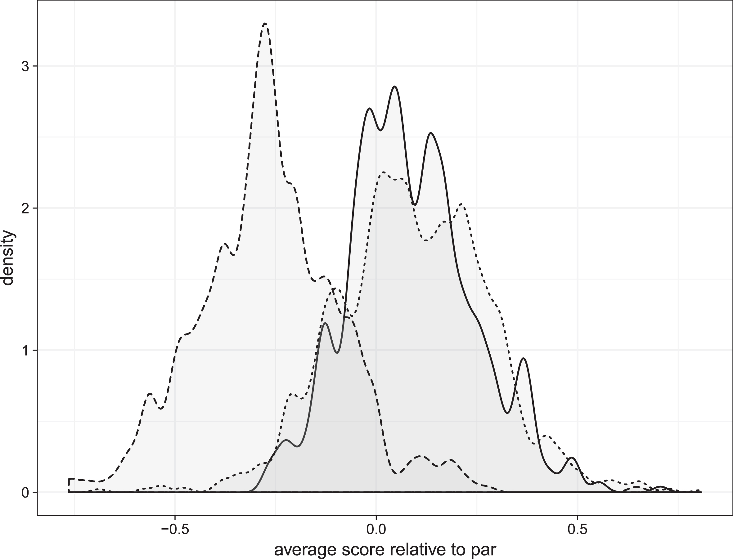
The par on a given hole is a rating that is arbitrarily designated by the course, generally related to the length of the hole and little to do otherwise with the relative difficulty when compared to holes of similar length. It is not unheard of at some tournaments for a particular par 5 to actually have a lower stroke average than a particular par 4. Livingston (2012) normalized the scores across holes to a par 4 score in order to compare the scoring averages across the tours. We illustrate a similar normalization of scores in our sample in Fig. 1. Given that the distribution of normalized scores on par 5 holes is quite different from those of the par 3s and par 4s, we will adjust our predictions with a par-type fixed effect in our subsequent development. For completeness, for the top 177 players listed on the PGA Tour website for the 2014 season, the Par 3 scoring average was 3.065 PGA Tour (2016a), the Par 4 scoring average was 4.051 PGA Tour (2016b), and the Par 5 scoring average was 4.677 PGA Tour (2016c).
Fig. 1.
The distributions of average score (strokes) relative to par by par type. The solid line, short dashes, and long dashes represent the distributions on Par 3s, 4s, and 5s, respectively.
2Methods
In order for us to quantify a “hot hand” or “cold hand” effect, we consider the following variables/factors as the basis of our model, as well as potential interaction effects.
1. How difficult is a hole playing on a given day?
2. What was the player’s result on the previous hole?
3. Who is playing the hole (random effect)?
4. What is the difficulty rating of the hole, i.e. the par on the given hole?
The first question is computed in order to quantify the day-to-day difficulty of golf holes. That is, a par 5 could be playing particularly difficult one day with an average score of 5.2, and the next day the same hole could be averaging 4.9 strokes. This provides more information related to the hole’s relative difficulty rather than just calling it a par 5 both days. We will simply compute the field’s average score for a given hole as a measure of hole strength. The second question simply refers to whether or not a BoB (or BoW) was recorded on the player’s prior hole.
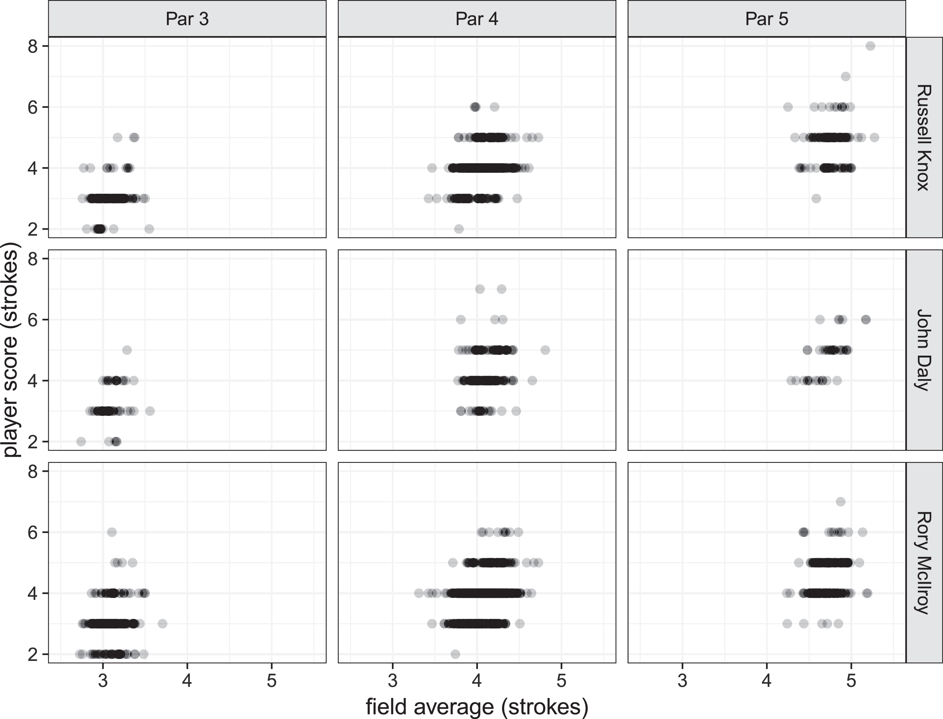
In order to answer the third point, we start by examining how each player performed on each hole relative to the field. Let us consider Rory McIlroy. Russell Knox, and John Daly to illustrate our point and overall calculations. It should be noted that McIlroy and Knox were the 1st and 100th rated players, respectively, as of December 28, 2014, and John Daly was above 300 (see OWGR (2014)). For each player, Fig. 2 shows their actual scores plotted against the field averages for each hole that they played in our sample. Note that the results are displayed according to the actual par on each hole, i.e. Par 3, 4, or 5. This figure indicates that Rory McIlroy tends to make a BoB (BoW) more (less) often than Russell Knox and John Daly, which is of course not surprising given their respective rankings.
Fig. 2.
The field average for all holes played by Rory McIlroy and Russell Knox versus what each player actually recorded on those holes.
2.1Statistical model
In order to test for a birdie or better (bogey or worse) effect, we employed the following random effects logistic models. Letting k denote the specific scenario of interest (i. e., birdie or better or bogey or worse), the models take the generic form2 given by
(1)
logit(π(k)ij)=log(π(k)ij1-π(k)ij)=x′(k)ijβ(k)+z′(k)iζ(k)iwhere i = 1, 2, …, 213 is the player index and j = 1, 2, …, ni represents the number of holes played per player, in chronological order3 In this formulation, we omit a tournament index and re-emphasize the fact that the initial hole in a given round is never used in our analysis as it is impossible to record a BoB (BoW) prior to this hole. The vectors x(k)ij and z(k)i of the fixed and random effect variables, respectively, for the BoB and BoW models. The specific covariates considered are: X1 = field average normalized by the hole’s par rating, X2 = birdie or better (or bogey worse, depending on k) on the previous hole, X3 = an indicator for par four holes, and X4 = an indicator for par five holes, with par three holes as our reference category. We considered a random intercept and slope parameters as our player-specific random effects.
For completeness, we make the usual distributional assumptions that govern models of the form given in Equation 1. That is, we assume Y(k)ij|π(k)ij∼Bernoulli (π(k)ij)) where π(k)ij=P(Y(k)ij=1|x(k)ij,ζi) and ζi has either a univariate or multivariate normal distribution depending on the random effects specification.
2.2Model selection
In order to select a “best” models out of a host of candidates, we relied on the Akaike Information Criterion (AIC) (Akaike, 1974) and the Bayesian Information Criterion (BIC) (Schwarz, 1978). We will describe the overall process for choosing our model related to the birdie or better problem and note that the process is similar when considering bogeys or worse.
Recall that the basic problem amounts to determining if a PGA Tour player is more likely to record a BoB immediately after having recorded a BoB on the prior hole than if they scored a par or worse. Therefore, our dependent variable is a binary variable recording BoB (1) or par or worse (0). As mentioned in the previous section, the specific covariates considered are: X1 = field average normalized by the hole’s par rating, X2 = birdie or better (or bogey worse, depending on k) on the previous hole, X3 = an indicator for par four holes, and X4 = an indicator for par five holes, with par three holes as our reference category. The initial models in each scenario (k = {BoB, BoW}), contained all two-term interactions and lower-order terms as fixed effects. In addition, we included a random intercept term for each player and random player-specific slope components for each fixed effect. Given that this set of variables was not overwhelmingly large, we dropped terms sequentially, refit the reduced models, and recorded the model’s AIC and BIC. We did this until we arrived at the lowest AIC and BIC levels, and were satisfied with a parsimonious and interpretable model. The results are presented and discussed in the Results Section.
2.3Power analysis
A common, and we would argue justifiable, criticism of hot hand research is that the studies are underpowered. That is, the statistical methodology being employed is not able to detect an effect even if one were to exist. Several factors can contribute to underpowered analyses, however, it is often a result of small sample sizes. This phenomenon is discussed at length in Green and Zwiebel (2017).
Given these criticisms, we conducted a large-scale Monte Carlo simulation in order to determine effect sizes that we could reasonably detect given the make up of our data set. In this study, we define effect size as the difference between the baseline probability of BoB (or BoW) and the probability of BoB (or BoW) given a BoB (or BoW) on the player’s previous hole.
In order to estimate the power in detecting a BoB4 effect we randomly generated new indicators of BoB for each observation in our original sample. Overall, the estimated probability (p) of BoB on a par 3, a par 4, and a par 5 hole in our sample is 0.127, 0.152, and 0.385, respectively. Therefore, for each player on each hole played, we generated a random Bernoulli observation with probability (p) defined by the hole’s par rating to indicate whether or not a BoB was hypothetically recorded. On holes immediately following a BoB, we generated Bernoulli observations having probability of BoB given by p + δ where delta varied from 0.002 to 0.02. We refer to δ as the “effect size”.
The model used in our Monte Carlo study is an oversimplification of the model that we defined in Equation 1 in that we do not account for player-specific random effects in the data generation process. That is, we fit the model given by
(2)
logit(πij)=log(πij1-πij)=x′iβwhere xij includes fixed-effect terms for a hole’s difficulty on a given day x1, indicator variables for par 4 (x2) and par 5 (x3) holes, and an indicator variable for BoB on the previous hole (x4). Therefore, our focus is on testing the significance of the parameter associated with x4 at the α = 0.05 level of significance.
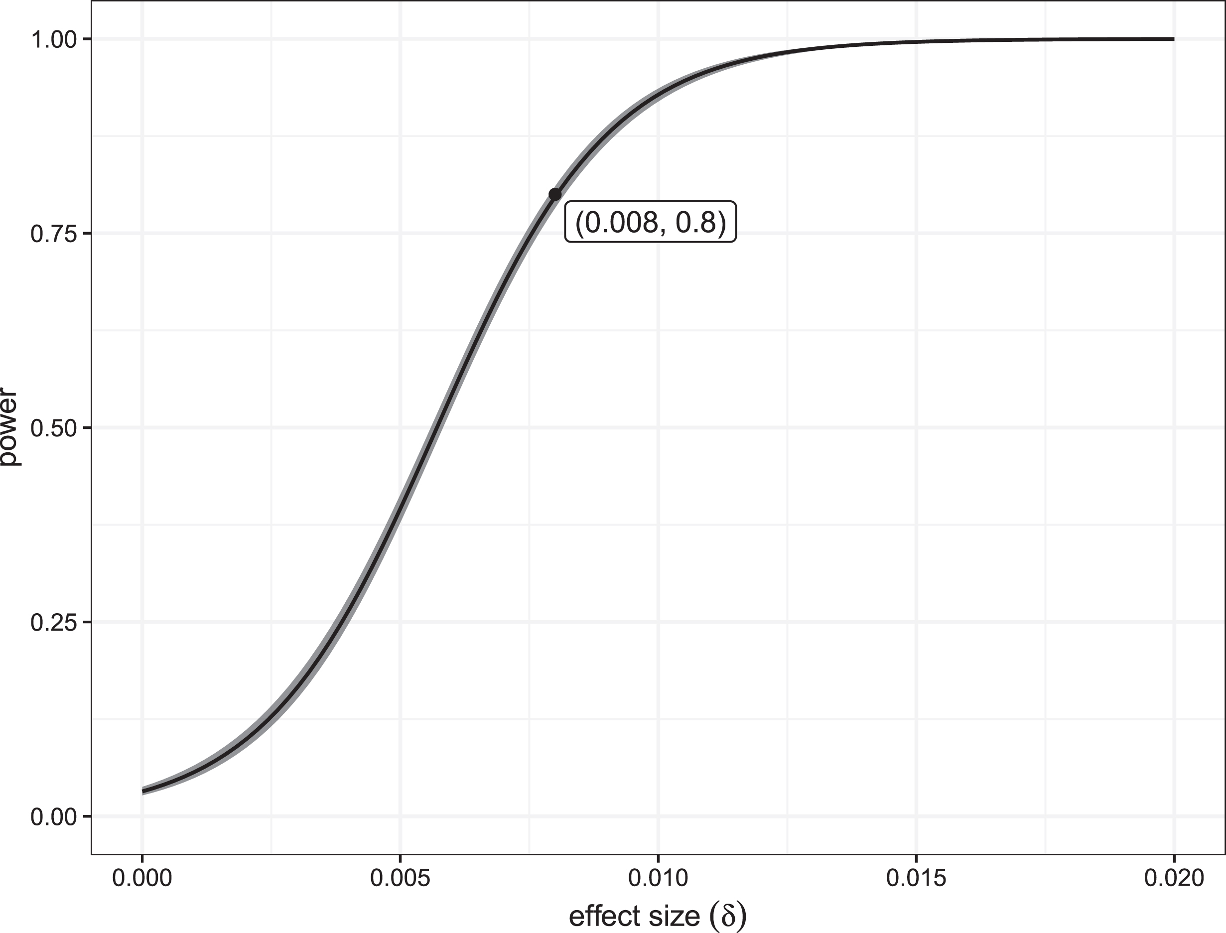
The estimated probabilities of detecting a significant difference as a function of effect size, or δ, is given in Fig. 3. We highlight the point (0.008, 0.8) as this is the minimum detectable effect size at the α = 0.05 level of significance. If, for example, the true probability of BoB is p = 0.127 (par 3s), we have a 0.80 probability of detecting if the probability of BoB immediately following a BoB changes to p = 0.135 or greater. A similar result holds for par 4s and par 5s. Finally, we note that the power function increases rapidly and we are virtually guaranteed to detect any effect size (δ) greater than 0.015.
Fig. 3.
The estimated power of detecting a hot (cold) hand effect as a function of effect sizes ranging from 0 to 0.025.
3Results
3.1Hot hand effect
As mentioned in Section 3.1, we fit a series of candidate models and selected the “best” fitting model according to AIC/BIC. Our primary hypothesis of interest is the following: PGA Tour players have a higher probability of recording a birdie or better on the hole immediately following a birdie or better, relative to when their previous hole was a par or worse. Unfortunately, our analysis suggests that there is not enough evidence to make such a claim. We did find significant evidence to support the inclusion of a player-specific random slope (par type) and intercept effect, as well as significant normalized average strokes per hole and par type, see Table 2. As we mentioned earlier in this manuscript, the standard errors associated with regression parameters are often attenuated when not accounting for significant random effects. Perhaps the inclusion of random effects in the BoB analysis, we lose the ability to detect a significant prior hole success factor.
Table 2
The final BoB model summary of the fixed effect terms
| Estimate | Std. error | z stat. | p-value | |
| Intercept | -1.740 | 0.021 | -84.672 | 0.000 |
| Avg. diff. | -3.239 | 0.049 | -65.642 | 0.000 |
| Par 4 | 0.173 | 0.023 | 7.477 | 0.000 |
| Par 5 | 0.344 | 0.031 | 10.942 | 0.000 |
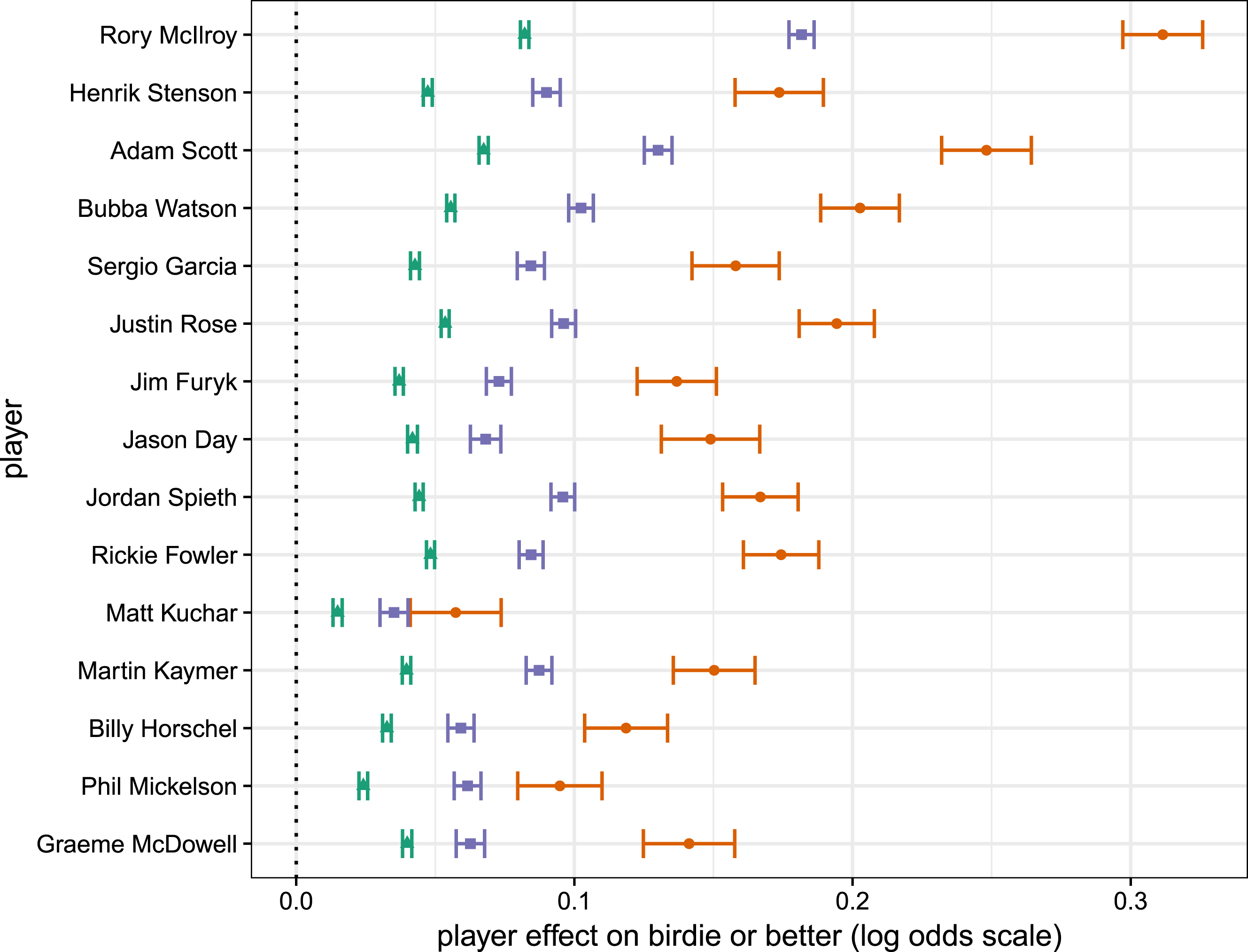
Despite the unsatisfying result mentioned above, there were several positive results related to this modeling exercise, for example, the need to include player-specific random effects. This allows us to confidently estimate the probability of a player in our sample recording a birdie or better on any hole given its par type and how difficult it is playing. Similarly, we can compare players across holes with respect to their probability of making a birdie or better. We illustrate such a comparison in Fig. 4. The figure shows the player-specific contributions to the probability of recording a BoB on Par 3s (purple), 4s (green), and 5s (orange) for each of the Top 15 players in the Official World Golf Rankings as of December 28, 2014. Rory McIlroy was ranked 1, Henrick Stenson 2, and Graeme McDowell 15 during the season under study. This figure very clearly shows just how dominant Rory was during the (at this point) peak of his career.
Fig. 4.
The player-specific intercept terms associated with each par type (3 - green, 4 - purple, and 5 - orange) on recording a birdie or better (log odds scale) for each of the top 15 players in Official World Golf Rankings during the time under study.
3.2Cold hands
Similar to our hypothesis given in Section 4.1, we are primarily interested in the following: Do PGA Tour players have a higher probability of recording a bogey or worse on the hole immediately following a bogey or worse, relative to when their previous hole was a par or better? The final model in this case results in a significant player-specific intercept, as well as significant fixed effect terms related the difficulty of the hole (average score relative to par), par type, and whether or not a bogey or worse was recored on the prior hole. The overall contribution (on a log odds scale) for the prior hole BoW effect is 0.093 (s = 0.021), as shown along with the other fixed effect estimates in Table 3.
Table 3
The final BoW model summary of the fixed effect terms
| Estimate | Std. error | z stat. | p-value | |
| Intercept | -1.820 | 0.020 | -90.569 | 0.000 |
| Avg. diff. | 3.117 | 0.047 | 66.260 | 0.000 |
| BoB prev. | 0.093 | 0.021 | 4.474 | 0.000 |
| Par 4 | 0.086 | 0.019 | 4.429 | 0.000 |
| Par 5 | 0.376 | 0.033 | 11.480 | 0.000 |
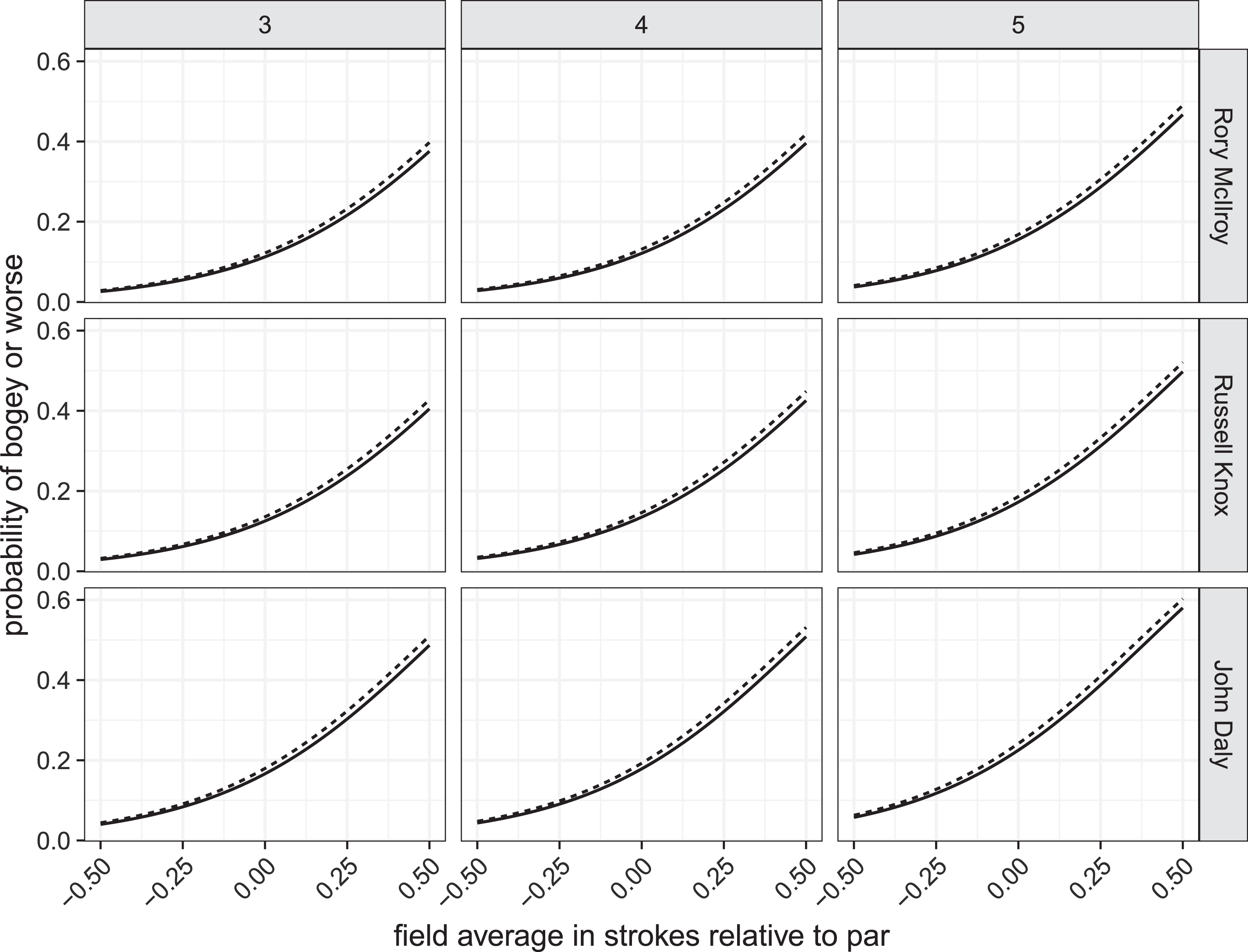
In order to visualize this effect, we plot the probabilities of recording a bogey or worse on various par types and difficulties for three players in this study: Rory McIlroy (ranked 1), Russell Knox (ranked 100), and John Daly (ranked above 300). The probability curves are shown for when a player records a bogey or worse on the prior hole (dashed line) versus when the player did not (solid line). Note that although the effect of scoring a BoW on the next hole is fairly consistent across players (difference between solid and dashed lines), the individual player curves are different in their respective magnitudes. In particular, Rory is less likely to record a BoW on the difficult holes regardless of the hole’s par rating.
Fig. 5.
The probability of birdie or better as a function of field average relative to par on different par types by Rory McIlroy (ranked 1), Russell Knox (100), and John Daly (>300). The solid lines represent the baseline probability of a bogey or worse and the dashed line represents the adjustment for recording a bogey or worse on the previous hole.
4Discussion
In this paper, we present a new approach to the well-studied hot and cold hand topic using a data set from the 2014 PGA Tour. Specifically, we used logistic regerssion models with player specific random effect components to estimate the probability of recording a birdie or better and a bogey or worse based on a host of hole and game attributes. In particular, we tested for hot and cold hand effects by including a prior hole result as an attribute in our model development.
Our results are consistent with the majority of the hot-hand literature (i.e., it is hard to find evidence in support of a hot hand), we do find evidence in support of a PGA Tour wide cold hand effect. That is, PGA Tour players, on average, are significantly more likely to record a bogey or worse immediately following a hole in which he recorded a bogey or worse, rather than when a par or better was attained. These results point to the notion that PGA Tour players have, perhaps, a harder time “letting go” of a negative outcome than they do in building off of their positive results.
In addition to our main hot and cold hand results, we use the final BoB to estimate individual player differences with respect to their probability of recording a birdie or better across different types of holes. And, as was mentioned, this follow-up analysis illustrates just how great Rory McIlroy was during this season.
Finally, we mention, again, that all of the prior studies on this topic, regardless of sport domain, focus on a fixed-effects-based analysis and neglect the intra-subject correlation that is inherent to repeated measures on the same individual. As mentioned previously, this omission can lead to artificially inflated effect sizes due to the attenuation of their respective standard errors.
Notes
1 Subsequent to the analysis presented here, the authors were made aware of the PGA Tour’s Shotlink database. This DB contains all of the data that we used, as well as a wide range of additional attributes that are measured on each shot.
2 We intentionally write Equation 1 in its full generality due to the fact that our final BoB and BoW are comprised of a different set of terms.
3 We recognize that an ordered logit (or probit) could be employeed in this analysis, however, we intentionally chose the more parsimonious form in order to simplify the interpretation of the resulting parameter estimates. The overall conclusions would not change under either model formulation.
4 Note that a similar simulation could be constructed for BoW using p = 0.187, 0.205, and 0.105 for pars 3, 4, and 5, respectively.
Acknowledgements
The authors would like to thank Keith Christensen and David Lee for their assistance in the data collection process.
Appendices
Appendix
Table 4
The complete list of tournaments in this study
| PGA Championship |
| Quicken Loans National |
| Deutsche Bank Championship |
| The Barclays |
| Zurich Classic of New Orleans |
| WGC Bridgestone Invitational |
| TOUR Championship presented by Coca-Cola |
| AT&T Pebble Beach National Pro-Am |
| Northern Trust Open |
| The Masters |
| BMW Championship |
| CIMB Classic |
| THE PLAYERS Championship |
| Wells Fargo Championship |
| HP Byron Nelson Championship |
| U.S. Open |
| The Open Championship |
| World Golf Championship - HSBC Champions |
| The Greenbrier Classic |
References
[1] | Akaike, H. (1974) , A new look at the statistical model identification, IEEE transactions on automatic control, 19: (6), 716–723. |
[2] | Arkes, J. (2016) , The hot hand vs. cold hand on the PGA tour, International journal of Sport Finance, 11: (2), 99. |
[3] | Bar-Eli, M. , Avugos, S. and Raab, M. (2006) , Twenty years of hot hand research: Review and critique, Psychology of Sport and Exercise, 7: (6), 525–553. |
[4] | Bocskocsky, A. , Ezekowitz, J. and Stein, C. (2014) , The hot hand: A new approach to an old ‘fallacy’. In 8th Annual MIT Sloan Sports Analytics Conference. |
[5] | Clark III, R.D. (2002) , Do professional golfers choke? Perceptual and Motor Skills, 94: (3c), 1124–1130. |
[6] | Clark III, R.D. (2004) , Do professional golfers streak? A hole-to-hole analysis, ASA Section on Statistics in Sports, 3207–3214. |
[7] | Clark III, R.D. (2005) a, An analysis of players’ consistency among professional golfers: A longitudinal study, Perceptual and motor skills, 101: (2), 365–372. |
[8] | Clark III, R.D. (2005) b, Examination of hole-to-hole streakiness on the PGA tour, Perceptual and motor skills, 100: (3), 806–814. |
[9] | Clark III, R.D. (2005) c, An examination of the “hot hand” in professional golfers, Perceptual and motor skills, 101: (3), 935–942. |
[10] | Connolly, R.A. and Rendleman R.J. Jr. , (2008) , Skill, luck, and streaky play on the PGA tour, Journal of the American Statistical Association, 103: (481), 74–88. |
[11] | Cotton, C. , McIntyre, F. , Price, J. , et al. (2016) , Correcting for bias in hot hand analysis: Analyzing performance streaks in youth golf. Technical report. |
[12] | Csikszentmihalyi, M. (1991) , Flow: The psychology of optimal experience, volume 41: . Harper Perennial New York. |
[13] | Gilovich, T. , Vallone, R. and Tversky, A. (1985) , The hot hand in basketball: On the misperception of random sequences, Cognitive psychology, 17: (3), 295–314. |
[14] | Green, B. and Zwiebel, J. (2017) , The hot-hand fallacy: Cognitive mistakes or equilibrium adjustments? Evidence from major league baseball. Management Science, 1–34. |
[15] | Heath, L. , James, N. and Smart, L. (2013) , The hot hand phenomenon: Measurement issues using golf as an exemplar, Journal of Human Sport and Exercise, 8: (2), S141–S151. |
[16] | Kahneman, D. (2011) , Thinking, fast and slow. Macmillan. |
[17] | Livingston, J.A. (2012) , The hot hand and the cold hand in professional golf, Journal of Economic Behavior & Organization, 81: (1), 172–184. |
[18] | NPR 2017, Cleveland Indians’ 15-game win streak means fans get $2 million in free windows. Last accessed 13 Nov 2017. |
[19] | OWGR 2014, Official world golf rankings. Last accessed 12 Feb 2017. |
[20] | PGA Tour 2016a, PGA tour statistics. Last accessed 31 Jan 2016. |
[21] | PGA Tour 2016b, PGA tour statistics. Last accessed 31 Jan 2016. |
[22] | PGA Tour 2016c, PGA tour statistics. Last accessed 31 Jan 2016. |
[23] | Rees, C. and James, N. (2006) , A new approach to evaluating “streakiness” in golf. In Proceedings of the World Congress of Performance Analysis of Sport VII, Szombathely, Hungary. |
[24] | Reifman, A. (2017) , Hot hand sports performance bibliography. Last accessed 13 Nov 2017. |
[25] | Schwarz, G. (1978) , Estimating the dimension of a model, The Annals of Statistics, 6: (2), 461–464. |
[26] | Scorsese, M. (Director). (1986) , The color of money. Touchstone Pictures. |
[27] | Young, J.A. and Pain, M.D. (1999) , The zone: Evidence of a universal phenomenon for athletes across sports, Athletic Insight: The Online Journal of Sport Psychology, 1: (3), 21–30. |

