
Three point shooting and efficient mixed strategies: A portfolio management approach
Abstract
Using mean/variance investment theory, we identify the efficient mixed shot type strategy for National Basketball Association (NBA) teams. The proportion of 3-point shots in this mixed strategy closely tracks risk and the change in expected points from 1979–2014. We then extend this approach to an individual team level for both offense and defense. This measures both the risk associated with implementing a mixed strategy (for and against an individual team) and the implied shot type efficiency for offense and defense. It is the latter, shot type efficiency, which predicts winning and winning point differential.
1Introduction
In any competitive sport, rules are put in place that are intended to control and influence the way players or teams compete. In basketball, rule changes are often made to influence how the game is played. For example, adding the shot clock in the National Basketball Association (NBA) in 1954 quickly changed the pace of the game, increasing scoring and ending stalling tactics. Basketball changed almost immediately as scoring went from 79.5 points per game in the 1954 season to 93.1 points per game in the 1955 season. Within 5 seasons, every team was averaging over 100 points per game. The rules changed and within 5 years, teams had all adapted and created a different, faster style of play. The change was not instantaneous because time is required to adjust tactics, personnel and training of basketball players to the shot clock. At that time, no basketball player would have been training with a shot clock in high school, college or in industrial leagues. The most profound change to the rules of American NBA basketball in recent decades has been the introduction of the 3-point shot. Again, the impact of the change was not immediate and the change is still affecting game strategy. Evidence of this is the fact that there has been an increasing trend for the percentage of 3-point shots used by teams in the NBA, increasing from virtually none (3.05 % to be precise) in the 1979-80 season when the shot was introduced in the NBA to 28.4 % in the 2015-16 season (see Fig. 1 below)1 Furthermore, the NBA Most Valuable Player award for both the 2015 and 2016 seasons was won by Stephen Curry, a skilled 3-point shooter. In this paper we analyze the adaptation of the game to the 3-point shot which in turn allows game outcome predictions to be made including where the game is headed in terms of aggregate two and 3-point shooting strategies.
Fig.1
Expected points from 2- and 3-point shots for the NBA as a whole.
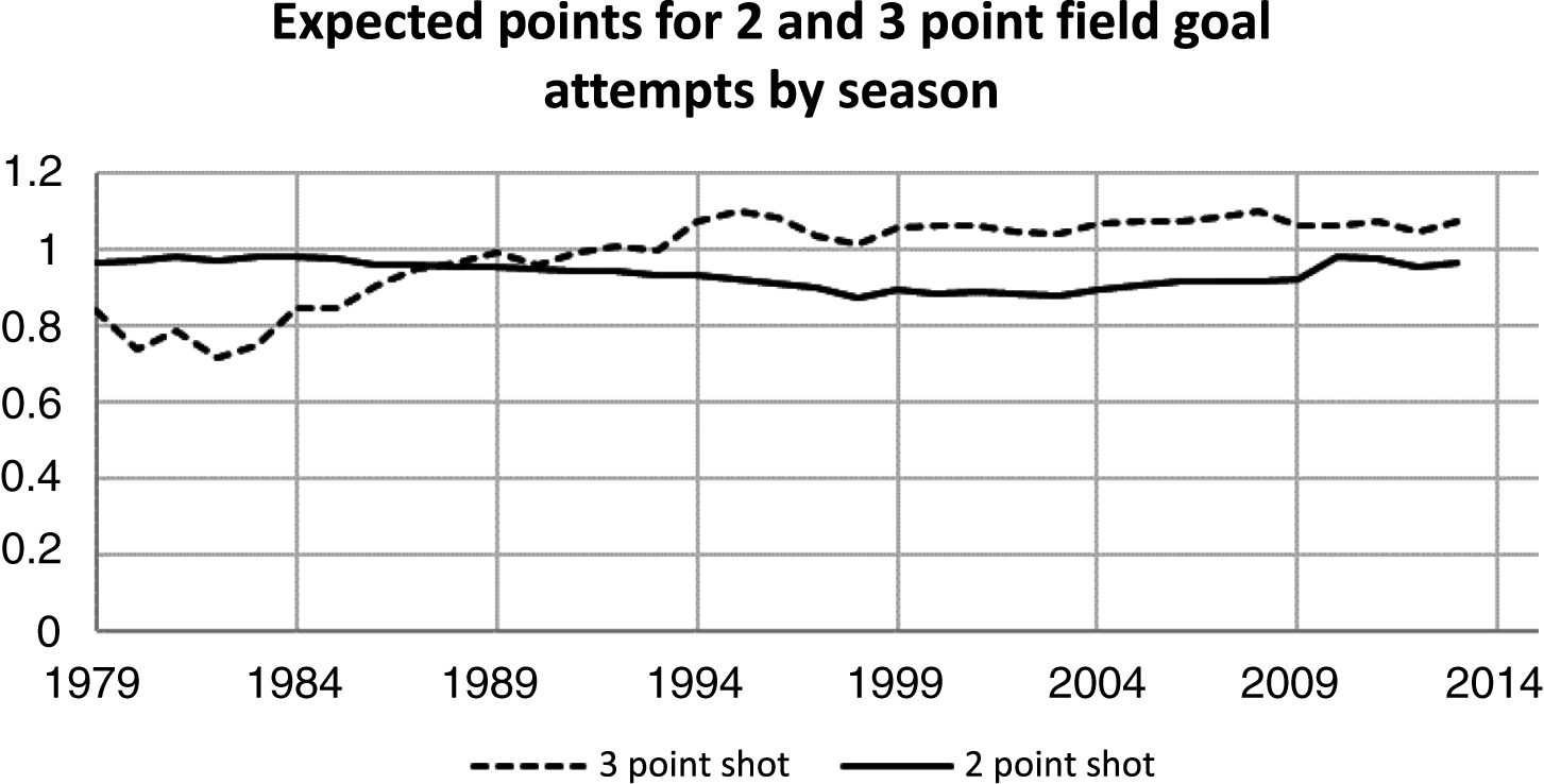
When analyzing 3-point shots, we first observe that both the mean and variance of the probability of a successful 2-point shot for the NBA have remained relatively stable over this time, whereas the probability of a successful 3-point shot has exhibited an increasing trend for its mean and a decreasing trend for its variance (See Fig. 2 below). Until 1987 the expected points from 2-point shots (2 points*probability of a successful 2-point shot) was higher than the expected points from 3-point shots. This reversed after 1987 up until current time (see Fig. 3). For the case of the variance of the probability of a successful 3-point shot, this has remained higher than the variance of the probability of a successful 2-point shot for the NBA each year, over the entire time period. This happens even though the variance of a successful 3-point shot has decreased over this same time period. Combined these observations suggest that not only the expected points from a shot type matters but also the variance or risk associated with a successful shot type matters. The latter follows because if only expected points from a shot type matter then we would observe 100% 3-point shots since 1987, which obviously did not happen. As a result, when making predictions about outcomes from NBA games, as well as describing shot type strategy, requires considering both risk and expected points from each shot type.
Fig.2
Risk Characteristics of 2 and 3-point shots for the NBA as a whole.
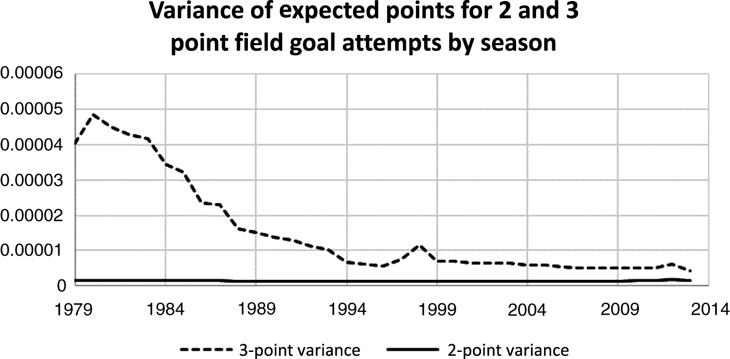
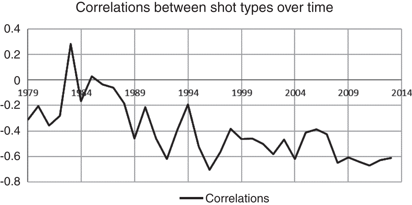
Fig.3
Correlations between Shot Types Made.
To formally analyze this problem, we adopt the finance approach of considering the mean, variance and covariance of expected payoffs from successful 2- and 3-point shots. That is, a team can treat their game strategy as a portfolio of shot types that have an associated risk and return. Our analysis draws heavily upon modern portfolio theory (MPT) and the Capital Asset Pricing Model (CAPM) to analyze NBA basketball strategy. Modern portfolio theory allows us to first explain and predict 3-point trends for the NBA as a whole and we find that the proportion of 3-point shots in this mixed strategy closely tracks risk and expected points changes for 3-point shots in the NBA from 1979–2014. We then shift attention to the individual team level by applying the CAPM to describe both the offensive and defensive strategies at a team level. This provides us with a pricing model for shot types at a team level for both offense and defense. The advantage of this approach is that the slope of the defensive and/or offensive shot type pricing models reveal whether a team can more easily (i.e., at lower cost) defend against and/or make 3-point shots. In turn these results can be applied to problems ranging from predicting post season success to developing a strategy when playing against a team as well as engineering an NBA team. In the current paper we focus upon the prediction issue. In all our analyses, we are asking, over the course of a game, what mixture of 2 and 3-point shots should a team try to achieve. We are not asking, on any particular possession, what type of shot a team should attempt. Rather, over a series of possessions such as a game or a season, what percentage of shots should be of eachtype?
This investment theory approach to identifying optimal mixed strategies also highlights the importance of risk aversion in the NBA. For example, professional golfers, playing for large prizes in golf tournaments, show evidence of loss aversion (Pope & Schweitzer, 2011). Professional football coaches, when making decisions about whether to ‘go for it’ on fourth down, show similar behavior (Romer, 2006). In both cases, golfers (who seem more sensitive to going over par (bogey) than to being under par (birdie)) and football coaches (who avoid the risk of failing to get a first down even when that is, in expectation, the more attractive option), players with high stakes reveal the influence of risk aversion upon their choice behavior. The NBA added a 3-point shooting line to the game in 1979, introducing a new and risky choice for coaches and players. The farther one is from the basket the greater the risk of not scoring. Prior to 1979, the NBA only had 2-point field goals. In 1979, after the NBA introduced the 3-point shot, only 3 percent of shots attempted were 3-pointers and the expected points from a 3-point shot was lower than the expected points from a 2-point shot. This reversed in 1986 such that expected points from 3-point shots exceeded the expected points from 2-point shots up to today. However, since 1986 the use of the 3-point shot has increased but does not dominate 2-point shooting as expected in a risk neutral world. This raises the several questions, such as:
“Currently in Europe it is quite customary to watch games where teams shoot more three-pointers than two-pointers. It will happen in the NBA, and soon.”2 Will it happen? While we do not answer this question, our framework provides a basis for suggesting whether it should happen.
In section 2 of this paper we motivate and apply mean/variance investment theory to basketball. That is, we analyze the relationship between the changes in the underlying statistical distributions generated from 2- and 3-point shot types over time with the observed proportions of 2- and 3-point shots taken over the same time periods. This relationship is used to both evaluate and predict performance. Finally, to make this evaluation concrete in terms of modern basketball terminology, we relate our economic variables to traditional basketball performance measures. From the perspective of existing sports analytical research in basketball our emphasis is on providing a game theoretic analysis of realized shot distributions, as opposed to studying within game behavior, as others have done (Goldman & Rao, 2012; Oliver, 2004; Skinner, 2012; Lucey et al., 2014). This work can be used to analyze shot distributions within a game, but we do not do that here and leave that task for future research.
2Efficient mixed basketball strategies
The game of basketball has two simple objectives for any team. The team wants to score points (offense) and prevent their opponent from scoring points (defense). The team that scores the most points wins the game. Associated with each shot type are expected points from making a successful shot and risk, because shots will either succeed or fail. The coach in any game has a strategic choice to make. How to play the game and what players to put on the floor to execute the coach’s strategy is the problem the coach needs to solve. Suppose the coach chooses to only shoot 2-pointers and puts players suited to that strategy on the floor and always plays to shoot near the basket. Then the other team’s defense would collapse near the basket and make success very difficult (i.e., ‘protecting the paint’). Suppose the coach chooses just to shoot 3-point shots? Then the defense adapts to that by crowding the 3-point line and making those shots as difficult as possible. The coach realizes the team needs a mixed strategy where the team shoots some 3-point shots and some 2-point shots. Now the coach has to ask, how many shots of each type should my team shoot? The choice the coach makes we define as the mixed strategy in thispaper.
NBA coaches and players understand this.
The analogous problem exists and has been solved in finance by analyzing the tradeoff between risk and return to identify the right combination of risky assets in an investment portfolio. The risks and returns are studied by first representing the returns from each risky asset in a mean/variance framework and then solving for the optimal portfolio weights relative to the investment objective. If return distributions change then so do the predicted portfolio weights. This is referred to as “modern portfolio theory” or MPT analysis. The same analysis is relevant and applicable to basketball by representing shot types in a mean/variance world. Here is an example. In 1994, the NBA moved the 3-point line closer to the basket (uniformly 22 ft. instead of 23 ft. 9 in.). As a result, the risk (i.e., variance) from taking 3-point shots was reduced, and expected points increased. Teams immediately started shooting significantly more 3-point shots, showing that the coaches were prepared to tradeoff risk and return. As the risk went down and the return increased, 3-point shooting took off. Three years later, the NBA moved the line back to 23 ft. 9 in. Coaches immediately responded to the increased risk created by this change, reducing the number of 3-point shots attempted. Modern portfolio theorists recognize this behavior as a rational, correct response to the changes in the mean and variance of returns from 2 and 3-pointshots.
2.1An economic analysis of basketball: An overview
In this paper we identify the efficient mixed strategy for the NBA in aggregate by maximizing the Sharpe Ratio (SR), which is defined here as the expected points divided by the volatility of points. The optimal proportion of 3-point shots for the NBA is then identified from the efficient mixed strategy.
We then extend this aggregate analysis to the individual team level. In this extension we identify the efficient mixed offensive and defensive strategies by maximizing the SR for each team in each year. The efficient mixed strategies are computed from the offensive (shots made) and defensive (shots given up) distributions. For offense a larger SR is preferred to smaller because this implies that the expected points per unit of risk is higher. The opposite applies to the defensive SR, because a smaller SR implies that the expected points per unit of risk is lower for the team playing against the defense. Finally from the efficient mixed strategy a shot type pricing model is derived for both offense and defense. This provides measures of the risk adjusted price of each shot type by team. An immediate advantage of applying this theory to basketball is that these results are scalable to any number of shot types. A team could analyze different shot types such as corner 3-pointers as compared to other 3-point locations as well as the relative return on midrange jump shots (from 15 feet where they are possibly riskier while only yielding 2 points as a return).
In summary, adopting the above economic analysis of basketball results in the following parameters:
(i) At an aggregate level the NBA’s efficient allocation of aggregate 2- and 3-point shots is estimated from 1979 to 2014.
(ii) At an individual team level an offensive 4-tuple: (Sharpe Ratio, 2-point beta, 3-point beta, and slope of Shot Market Line) for each team.
(iii) At an individual team level the defensive 4-tuple: (Sharpe Ratio, 2-point beta, 3-point beta, and slope of Shot Market Line) for each team.
From (i) above, the unique mixed strategy is compared to the NBA actual aggregate statistics for 2- and 3-point shots. For (ii) and (iii) the 4-tuples are estimated using within season data and then applied to predict post season performance. Finally, to better understand our measures and their relation to basketball performance, we correlate our parameters to the factors identified by Oliver (2004) as capturing offensive and defensive performance. This will identify the empirical relationships between these theoretical parameters with modern basketball performance measures.
We first consider some simple statistics that describe the phenomena being analyzed.
2.2Offensive investments: Allocation of shot attempts to 2 and 3-pointers
Expected points is points per shot times the probability of successful shot attempts for each shot type. In Fig. 1 this is plotted over time for 2- and 3-point offensive shots. If coaches employ a risk neutral strategy, this would imply that only 2-point or 3-point shots are taken. The graph in Fig. 1 suggests that, for risk neutral teams, only 2-pointers would be used up to 1987 (expected points are higher from 2-point shots up to 1987), followed by only shooting 3-pointers from 1988 on. Actual NBA shot data do not reflect this extreme risk neutral prediction with all 2-point shots crossing over to all 3-point shots. Figure 2 depicts the interesting behavior for the variance of successful 2- and 3-point shots each year. This reveals that 2-point shot variance has been relatively stable over time until recently whereas 3-point shot variance has been declining. If risk is important and we equate variance to risk, as the riskiness of a 3-point shot declines the 3-point shot should be taken more frequently. In fact, this has happened. This is further reinforced from the observation that both the mean and variance of points are also responsive to the rule adjustments made during the 1994–95, 1995–96 and 1996–97 seasons. As noted above, the NBA shortened the distance of the line from 23 feet 9 inches and 22 feet at corners to a uniform 22 feet from the basket. In 1997–98, the NBA then reverted back to the original distance of 23 feet 9 inches and 22 feet at the corners. Figures 1 and 2 indicate that both the mean and the variance are sensitive to these rule changes between 1994 and 1997.
One advantage of invoking the predictions from the optimal mixed strategy is that the NBA can predict the impact from changing rules upon shot taking behavior, which is especially important if maintaining a particular 2- and 3-point shot ratio for fans is an important objective. However, before being able to make such predictions there is a third input that influences predictions from the optimal mixed strategy. This is the covariance (or correlation) between 2- and 3-point offensive shot investments. By using each team as an observation within each year the 2- and 3-point shot expected points correlations can also be computed each year. Figure 3 plots the results from this analysis of the 2- and 3-point data across teams, computing a Pearson product-moment correlation coefficient.
Combined, Figs. 1, 2 and 3 provide the basic building blocks for identifying the efficient mixed strategy for basketball as formally described next.
2.3Identifying the Efficient Mixed Strategy
The set of efficient 2- and 3-point shot strategies is identified by maximizing the Sharpe Ratio, where j = 1 (2-point shots) and 2 (3-point shots) and the maximization problem is defined as follows:
(1)
Subject to:
Where
ω = a vector of shot type weights (α2, α3) the proportion of 2- and 3-point shots in the mixed strategy and sT the shot type points. Expected points from the mixed strategy is defined as:
For 2- and 3-point shots, the portfolio volatility (i.e., standard deviation) is: σ =
For the problem defined above in equation (1), p, the probability of a successful shot computed from n shots is a random variable estimated from the data (dropping shot type subscript for expositional ease). The distribution for p is estimated by applying the central limit theorem to the large number of both 2 and 3-points shots each season, and the variance of p is normally distributed and equal to p*(1-p)/n. As a technical aside, we do not define variance in terms of being a random variable from the Bernoulli distribution, which assumes it is the outcome from a sequence of shot realizations generated from the Binomial (n, p) distribution. This is because invoking the Bernoulli distribution assumes that p is a parameter, i.e., a fixed real number, as opposed to being itself a random variable which must be estimated from the data. Finally, we compute the Pearson correlation coefficient, r, between 2- and 3-point shots from each team’s total shot statistics per regular season year. By assuming each team makes a tradeoff between using 2 and 3-point shots in their offensive strategy, we calculate the Pearson correlation coefficient using each team as an observation. The number of teams used to estimate r, range from 22 NBA teams in 1979 to 30 NBA teams currently, and finally covariance is then defined as rσ2σ3.
The solution to the above maximization problem, when applied to NBA aggregate data, identifies the efficient mixed strategy of 2- and 3-point shots for the NBA as a whole. Here we define efficiency for offense as the mixed strategy that maximizes expected points per unit of risk. For the NBA as a whole this is also equivalent to finding the minimum expected points given up per unit of risk. That is, the offensive and defensive problems are symmetrical. However, this symmetry does not extend to individual teams and both offensive and defensive performances are measured and analyzed separately for individual teams as discussed next.
1. Individual Team Level of Analysis
The game of basketball consists of both offense and defense and therefore to analyze basketball at the individual team level we first apply equation (1) to identify the two efficient mixed strategies, offensive and defensive for each team. In this paper, we solve for the mixed strategy that maximizes the Sharpe ratio (e.g., Elton and Gruber (1995)), and refer to this strategy as the “Efficient Mixed Strategy” (EMS). Central to this theory of investment returns is the idea that higher risk is associated with higher expected returns in a world where risk aversion is important. By applying investment theory to basketball, we relate the expected points from the 2- and 3-point shot types to the risk associated with each shot type for each team. The steepness of this relationship provides insight into the cost associated with a team’s tradeoff between risk and expected points. Formally the CAPM theory predicts the following general form for this relationship, referred to as the Security Market Line (SML) which is positively sloped and defined as follows (e.g., Bodie, Kane and Marcus (2013)):
(2)
Shot type betas are estimated in two equivalent ways, relative to each team’s efficient mixed strategy. First, beta is defined as the covariance between the average shot type payoff and the optimal mixed strategy payoff, scaled by the variance of the optimal mixed strategy payoff. The efficient mixed strategy is computed from the variance/covariance matrix, where covariance is estimated by computing the correlation between shot types estimated from the 30 teams, multiplied by the product of the shot type standard deviations. Equivalently, and simpler, shot type betas can be computed directly from the ratio of the average payoffs relative to the efficient mixed strategy as described by Equation (2).
To make the above theoretical concepts concrete it is instructive to first illustrate some of the important statistics that this analysis produces by applying it to the first and last place teams in the regular 2013 season. This will help to focus on some of the intuition behind the empirical results that follow.
2.4Example: Miami compared to Orlando 2013
During the regular 2013 season Miami attained the highest win percentage of 80.48 percent and Orlando the lowest, 24.39 percent. Based upon regular season team results, the SR, shot type betas and SML slope, for Miami and Orlando is as follows:
Miami 2013 Regular Season Offensive Performance
Sharpe Ratio = 16.33
Beta (2-point) = 0.96
Beta (3-point) = 1.15
Slope of the Shot Market Line (SML) = 1.03
Miami 2013 Regular Season Defensive Performance
Sharpe Ratio = 13.79
Beta (2-point) = 0.96
Beta (3-point) = 1.14
Slope of the Shot Market Line (SML) = 0.91
Orlando 2013 Regular Season Offensive Performance
Sharpe Ratio = 13.34
Beta (2-point) = 0.98
Beta (3-point) = 1.08
Slope of the Shot Market Line (SML) = 0.91
Orlando 2013 Regular Season Defensive Performance
Sharpe Ratio = 13.54
Beta (2-point) = 0.97
Beta (3-point) = 1.12
Slope of the Shot Market Line (SML) = 0.96
Major differences immediately appear between these two teams both offensively and defensively which can be interpreted as follows.
Consider first the Sharpe Ratio (SR) which imposes a price of risk constraint upon the efficient mixed strategy. A high offensive (low defensive) SR is preferred to a low offensive (high defensive) SR because the offensive SR measures the expected points per unit of risk and the defensive SR measures the expected points given up per unit of risk. For the case of Miami versus Orlando, Miami has a higher price of risk for its offensive mixed strategies. As a result, Miami will have a higher expected points per unit of risk than Orlando in its efficient mixed strategy.
Additional insight into the drivers of the above differences is provided by considering both the offensive and defensive SML’s. The analogy to the Security Market Line for basketball can be interpreted as follows. In regular CAPM all risky assets are predicted to lie on the Security Market Line in equilibrium. For basketball each risky shot type is predicted to lie on the Shot Market Line (SML). In the above example the slope of the SML is constructed for both offense and defense. For the case of offense a steeper SML implies that the expected points per unit of risk is higher for the 3-point shot compared to the 2-point shot. In addition, the steeper the SML the stronger the offense. Recall from Fig. 2 that the variance of 2-point shots has remained relatively stable for about three decades whereas the variance of the 3-point shot has been declining. The CAPM theory predicts the shot type beta is a function of shot type volatility (e.g., Bodie, Kane and Marcus (2013)) and as a result, the steeper the SML the better is the offensive 3-point shooting from an expected points perspective relative to the 2-point shot type. This difference between CAPM applied to financial securities as opposed to shot types, is that for financial securities the expected return pricing model includes a risk free rate, typically non-zero, whereas for the basketball shot types, the offensive shot pricing model originates at the origin (i.e., risk free rate equals zero). In both cases, however, steeper rays dominate flatter rays. The opposite applies to the defensive SML as it is defined in terms of points given up. In the above example, Miami compared to Orlando reinforces these insights.
3Data
Data for team level analyses for the years 1979–2014 was extracted from data provided by databasebasketball.com3. In particular, we used the file team_season.csv which provides data on shots taken, shots made, and winning percentage at the team season level. For analyzing individual team performance and performance in the playoffs, we used game level data provided by nbastuffer.com for 2007–2014. We analyze team level NBA data starting in 1979. That is the year the NBA introduced the 3-point shot. The line is 23′ 9″ away from the basket excepting in the corners of the basketball court, where the distance is shorter (22 feet), again, excepting the 1994-95, 1995–96 and 1996–97 seasons, as discussed above.
4Application of the efficient mixed strategy theory to NBA basketball
The first problem we address at the aggregate level is to provide a theoretical explanation of the observed trends in the percentage of 3-point shot taking from 1979 to 2014 in terms of mean/variance efficient mixed 2- and 3-point strategies. This theoretical explanation provides a prediction for the NBA regarding what the future trend for percentage of 3-point shots is likely to be given current skill levels.
4.1Results for NBA as a whole
In this section we present the results from solving each year for the aggregate offensive efficient mixed strategy for the NBA as a whole. The analysis proceeds by constructing the distribution of points from each shot type for the NBA as a whole by year. Figures 1–3 above depict the evolution of the 3-point shot and its use in the mixed strategy, over time. The negative correlation between 2- and 3-point shot successes is pronounced and reinforces this evolving use of the 3-point shot in NBA strategies. For example, as noted by players such as power forward David Lee of the Golden State Warriors: “The game is changing,” Lee said, “and I think one of the things is not telling ‘4s’ (power forwards) they’re going to be in the post all the time. Instead, teams are giving them the option to shoot mid-range shots and threes. Then the defense has to make the adjustment.”4
As a result, as the mixed 2- and 3-point strategy becomes more prevalent, the negative correlation in Fig. 3 is becoming more pronounced. The efficient mixed 2- and 3-point strategies allow for a consistency relationship to be tested between the predicted efficient strategies each year and the actual observed outcomes. These results are depicted graphically in Fig. 4.
Fig.4
Actual versus Optimal 3-Pointers (Actual Correlations).
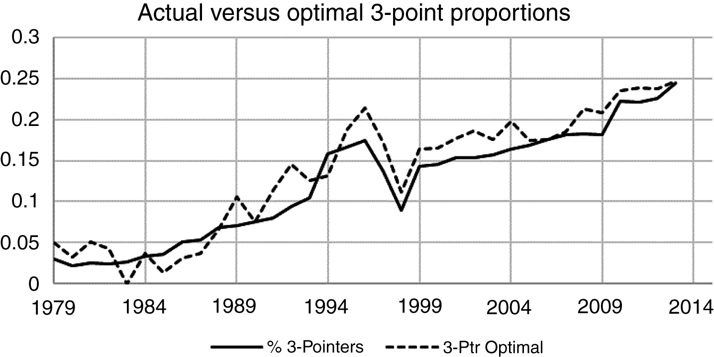
Figure 4 reveals that, in the aggregate, NBA coaches have exhibited highly efficient 2- and 3-point shot selection strategies. That is, there is a high level of consistency between aggregate mixed strategy behavior and player abilities when reduced to means, variances and covariances. It can also be observed that both actual and predicted behavior is sensitive to the rule changes that took place over the 1990’s. As a result, analytical modeling combined with empirical analysis of basketball can provide predictions for likely outcomes of future potential rule changes.
The above analysis also provides insight into where the NBA is headed in terms of predicted proportions of 3-point shots. Clearly, from a fan perspective, the NBA probably wants to maintain an attractive balance between the proportions of 2-point and 3-point shots in the game. In investment theory the variance and covariance of shot types are the major drivers of the predicted proportion of shots for a risk averse world. Although Fig. 2 reveals that the NBA has gone down a steep learning curve associated with the accuracy of the 3-point shot from 1979 to 1995, this learning curve settles down post 1995. Between 1995 and 1997 rule changes largely accounted for observed changes in 3-point accuracy and post 1997 the evidence suggests that team strategy became a major driver of this behavior. This is implied from the observation that the correlation between top shooters (in terms of accuracy) and top 3-point shooters (in terms of attempts) in 2014–2015 is substantially higher (r = 0.417) than it was in 1998–1999 (r = 0.329). One of the leading 3-point shooters today is Stephen Curry (accuracy = 0.443, third in the NBA in 2014–15). Coincidently, his father Dell Curry was the most accurate 3-point shooter in 1998-1999 (accuracy = 0.476). While Stephen Curry led the NBA in 3-point shot attempts, Dell Curry was not even among the top 20 players in 3-point attempts. Although overall league shooting accuracy has not changed very much, the significant overlap between high frequency 3-point shooters and the most successful 3-point shooters today implies that mixed strategies have taken time to evolve differently from just accuracy alone. This is also reflected in the greater stability of correlation trends between 2-point and 3-point shots over time. In order to tease out the relative impact of each of these two important inputs we can systematically introduce the correlation results into the analysis. In the next section we compare the actual versus predicted behavior in Fig. 4 when using estimated correlations versus a baseline case of zero correlation (i.e., independence).
First we consider the baseline case under the assumption of zero correlation between shot types. For this analysis we estimate the optimal mixed strategies under the imposed condition that the two shot type distributions are independent. This will allow the effects of shot accuracy (shot expected points variance) versus mixed strategy (shot expected points correlations) to be teased out by comparing Figures 4 and 5.
Fig.5
Optimal Number of 3-point shots versus actual under independence condition.
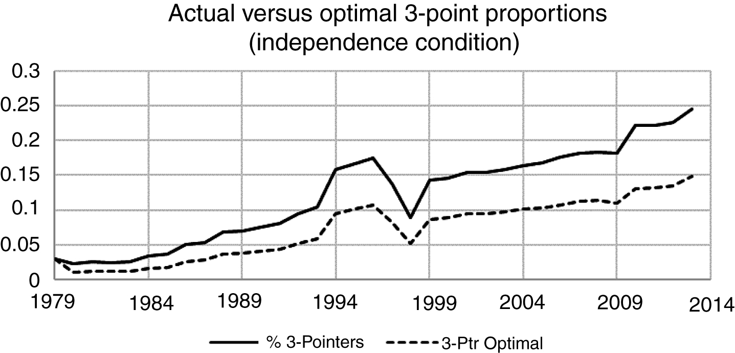
The results from Fig. 5 reveal that in aggregate for the NBA trends in the predicted efficient strategies are consistent with trends in Fig. 4 but the gap between actual and predicted is widening which demonstrates the increasing importance of mixed strategies in the game. The increasing widening of the two series is likely to be a result of the strategy learning curve that coaches and players in the NBA have been ‘going down’ over time that was alluded to by David Lee’s comments above. Figures 2 and 3 reveal that both variance and correlations have substantially stabilized in the last few years. This implies that it is unlikely that the proportion of 3-point shooting is about to dominate the proportion of 2-point shots as some have speculated will happen5.
Next, we extend the aggregate analysis of the NBA to the analysis of individual team performances during the regular season. The objective of this section is to provide a descriptive analysis of the basketball performance in terms of the team level performance measures identified from the theory. We analyze the dependent variable, win percentage, as a fractional response variable. For this fractional response, the values lie in the closed unit interval [0,1]. The linear probability model applied to such a dependent variable cannot guarantee predicted values will not fall outside the unit interval (Wooldridge, 2002). For this reason, other methods such as a log-odds transformation of the dependent variable and NLS estimation are often proposed. It has been shown that such estimators, while estimable with OLS, are problematic. In particular, they do not deal with values at the boundary, 0 and 1, and the regression estimators β are not easily interpreted (Wooldridge, 2002). Papke and Wooldridge (1996) propose a method to address this problem. They show that using a generalized linear model with a Bernoulli log-likelihood function and robust estimates of the standard errors provides estimates that are efficient, allow for values at the unit interval boundaries of 0 and 1, and are directly interpretable. For these reasons, we apply the method proposed by Papke and Wooldridge (1996). In our estimates, we use the logit cumulative density function.
The results from Table 1 reveal that each year’s descriptive model fits the data well. Furthermore, from inspection of the individual coefficients the pair of offensive and defensive SML slopes each had significant t statistics at or around the 0.001 level with signs in the predicted directions. When we aggregate the data from 2007–2014, and estimate the model with fixed effects for year and team, we find all 4 offensive measures are likely to have an effect, while only the defensive SML has an effect over the 8 seasons, comprising 240 team seasons. In all these cases the models fit the data reasonably well, but the models are only descriptive, given they are estimated on the same within season data used to estimate the predictors themselves. Later even more insight is provided when we relate the set of economic variables identified by the theory to traditional basketballfactors.
Table 1
Fractional regression models predicting regular season winning percentage using CAPM measures
| 2007 | 2008 | 2009 | 2010 | 2011 | 2012 | 2013 | 2014 | 2007–2014 | |
| Constant | 29.724 | 18.495 | 29.887 | 66.69*** | –54.419 | 25.147 | 11.761 | 2.609 | 22.364** |
| (18.986) | (22.549) | (19.990) | (20.275) | (30.201) | (22.493) | (16.497) | (8.427) | (9.419) | |
| Offense | |||||||||
| SML | 6.307** | 8.849*** | 8.54*** | 8.03*** | 10.36*** | 10.8*** | 10.06*** | 9.769*** | 9.81*** |
| (2.238) | (1.718) | (2.311) | (1.296) | (1.799) | (2.621) | (1.659) | (1.117) | (0.792) | |
| Sharpe Ratio | 0.045 | 0.056 | 0.091** | 0.015 | 0.139*** | –0.007 | 0.072 | 0.024 | .048** |
| (0.048) | (0.067) | (0.037) | (0.059) | (0.038) | (0.064) | (0.050) | (0.035) | (0.019) | |
| β2 | –18.36 * | 8.985 | –10.972 | –24.689 | 3.384 | –5.303 | 4.378 | 6.041 | –9.359 * |
| (9.003) | (10.583) | (5.856) | (13.095) | (9.790) | (10.145) | (7.688) | (3.983) | (4.198) | |
| β3 | –5.494* | –0.195 | –6.77 *** | –7.592 | –0.098 | –2.090 | omitted | omitted | –4.16 *** |
| (2.428) | (2.689) | (1.812) | (4.295) | (3.710) | (4.276) | omitted | omitted | (1.239) | |
| Defense | |||||||||
| SML | –13.98*** | –19.66 *** | –18.440 | –16.13 *** | –9.26 *** | –10.33 *** | –9.94 *** | –16.84 *** | –14.27 *** |
| (2.015) | (3.114) | (1.935) | (1.968) | (2.746) | (3.027) | (2.195) | (1.874) | (1.239) | |
| Sharpe Ratio | 0.075 | 0.0989 | –0.035 | 0.090 | –0.098 | 0.084 | –0.058 | 0.078 | 0.020 |
| (0.073) | (0.069) | (0.053) | (0.069) | (0.087) | (0.092) | (0.068) | (0.051) | (0.025) | |
| β2 | 0.771 | –17.606 | –3.868 | –18.687 | 36.950 | –19.72 ** | –14.272 | –3.280 | –5.931 |
| (10.575) | (13.978) | (11.957) | (10.390) | (19.089) | (8.389) | (11.398) | (7.089) | (5.330) | |
| β3 | –0.726 | –1.512 | 0.720 | –8.756 *** | 12.301* | omitted | –2.211 | omitted | 0.324 |
| (2.691) | (3.663) | (2.378) | (3.018) | (5.720) | omitted | (3.039) | omitted | (1.338) | |
| N | 30 | 30 | 30 | 30 | 30 | 30 | 30 | 30 | 240 |
| Fixed effects Year | No | No | No | No | No | No | No | No | Yes |
| Fixed effects Team | No | No | No | No | No | No | No | No | Yes |
| Log pseudo likelihood | –13.223 | –12.936 | –12.726 | –12.944 | –12.972 | –13.0113 | –13.137 | –12.961 | –103.852 |
| AIC | 1.482 | 1.462 | 1.448 | 1.463 | 1.464 | 1.408 | 1.409 | 1.331 | 1.24 |
| Pseudo-R2 | 0.777 | 0.821 | 0.913 | 0.837 | 0.834 | 0.745 | 0.741 | 0.856 | 0.833 |
*p < 0.05, **p < 0.01, ***p < 0.001. The regressions are all predicting team winning percentage using the fractional regression method discussed in the text.
4.2Out of Sample Analysis using the Post Season Championships
For the out of sample tests, the post season results from 2007 to 2014 were pooled to increase the sample size at the team level. In each year, the NBA champion is determined by a 16-team single-elimination tournament. The winner in each round in the tournament is the winner of a best-of-seven series. The tournament starts a few days after the end of the regular season. No adjustments to personnel occur between the regular season and post season. The loser of each best of 7 series exits the tournament. Given 16 teams, there are 15 series per year in each of the 7 years. The average series length is 5.6 games. The average annual tournament, composed of 15 series, has 83.8 games. Our analysis is at the game level. We use two dependent variables, (1) whether the home team won and (2) the point difference between the home team and road team. The predictor variables are offensive and defensive SML slopes, 2 and 3-point betas, and Sharpe ratios for the home team and the road team. In addition, year of the playoff and series (since games are nested under each 7 game series) are treated as random effects. We choose to use random effects for several reasons. We do not expect year to year variation to be systematically correlated with the effects of the predictors, so year to year variation is treated as random. Each series involves a set of games between the same teams. The observations within a series may be correlated. For this reason, observations within a series are modeled as random effects (Wooldridge, 2002; Angrist & Pischke, 2009).
These prediction models are multilevel models because you have games nested in series and series nested in year. We used the Stata command ME (multilevel estimation) to estimate the models. The first model, predicting the winner of a game in a series was estimated as a logit model using maximum likelihood. The logistic regression results for home game won are presented in Table 2. The fit is significant (Wald χ2 = 50.35, p < 0.001). The results again reinforce the descriptive within season analysis, and it is the offensive and defensive SML slopes that drive the results.
Table 2
Playoff performance predicted by CAPM measures
| Home Team winning | Home Team point differential | |
| Constant | 36.379 | –82.623 |
| (55.969) | (312.067) | |
| Road Team offense | ||
| Sharpe ratio | 0.044 | 0.075 |
| (0.088) | (0.489) | |
| SML | –7.972** | –68.998*** |
| (3.147) | (17.6) | |
| β2 | –14.628 | 57.49 |
| (17.649) | (126.182) | |
| β3 | –4.16 | –19.989 |
| (4.968) | (27.711) | |
| Road Team defense | ||
| Sharpe ratio | –0.256** | –1.58** |
| (0.1) | (0.56) | |
| SML | 14.616*** | 95.61*** |
| (4.343) | (23.99) | |
| β2 | –24.433 | 57.49 |
| (22.754) | (126.182) | |
| β3 | –4.435 | 22.513 |
| (6.175) | (33.939) | |
| Home Team offense | ||
| Sharpe ratio | 0.005 | –0.119 |
| (0.087) | (0.49) | |
| SML | 11.268*** | 70.816*** |
| (3.147) | (17.485) | |
| β2 | –8.168 | –55.964 |
| (18.141) | (100.385) | |
| β3 | –2.954 | –15.49 |
| (5.109) | (28.285) | |
| Home Team defense | ||
| Sharpe ratio | –0.065 | –0.389 |
| (0.1) | (0.559) | |
| SML | –11.167** | –60.347** |
| (4.365) | (23.964) | |
| β2 | 19.804 | 123.33 |
| (22.116) | (124.803) | |
| β3 | 0.995 | 39.261 |
| (5.92) | (34.072) | |
| Year of Playoff Game (df = 8) | –17.76 | 7.38E-08 |
| (5.88E05) | (7.46E-07) | |
| Series (df = 120) | –19.47 | 2.16E-08 |
| (4.55E07) | (4.83E-09) | |
| N | 670 | 670 |
| Log Likelihood | –400.338 | –346.895 |
| Wald χ2 | 50.35*** | 77.92*** |
*p < 0.05, **p < 0.01, ***p < 0.001. For the point differential estimates, we estimate a restricted maximum likelihood.
Next a more sensitive dependent variable, point differential, was analyzed to take into account the closeness of the game result. The prediction model for point differential is a multilevel mixed (having some fixed and some random effects) linear regression model that requires restricted maximum likelihood estimation. Restricted maximum likelihood first estimates the fixed effects and then estimates the random effects. The random effects are estimated with maximum likelihood without the fixed effects (Harville, 1977). The results are provided in Table 2. The linear regression of the point differential is significant (Wald χ2 = 77.92, p < 0.001). Again this analysis reinforced the same SML slope results where the four SML slope coefficients (offensive, defensive, home and away) are all highly significant (p < 0.01). The major conclusion from the individual team performance analysis is that SML slopes (offensive and defensive) are useful predictors of performance.
4.3Linking the Economic Variables to Basketball
In a popular and influential book, Oliver (2004) identifies four factors that determine success in the NBA. These are ranked as follows in terms of assessed order of importance for winning a game. The ranking is, Shooting, Turnovers, Rebounding and Free Throws per shot. In addition, the factors can be applied to both offense and defense. The variables for both offense and defense are:
• EFG% –Effective Field Goal Percentage which is adjusted for the fact that a 3-point field goal is worth one more point than a 2-point field goal.
• TOV% –Turnover Percentage which is an estimate of turnovers committed per one hundred plays.
• ORB% – Offensive Rebound Percentage which is an estimate of the percentage of available offensive rebounds a player or team grabbed.
• FT/FGA – Free Throws Per Field Goal Attempt.
It is useful to know how these four factors relate to the 4-tuple of economic variables identified in section 2 and we explore these relationships in a correlational analysis. It is noted however, that the four variables identified in our current paper’s economic analysis are derived from a coarse data set containing only 2- and 3-point shot distributions for both offensive and defensive performance. Refining the set of shot types as improved datasets become available in the future is likely to improve this type ofanalysis.
The results are provided in Table 3 and three estimates immediately draw our attention. First, offensive SML slope is extremely highly correlated (0.891) with the EFG% which is considered to be the major driver of success. However, recall from our analysis it was both offensive and defensive SML slopes that are the critical success drivers. As a result it is interesting to observe the defensive correlations. The EFG% of the opponent team is highly correlated (0.817) with the defensive SML slope. This is consistent with the fact that the higher the defensive SML slope the higher the expected points from the opposing team playing against the defense. Similarly, the EFG% correlation with the defensive SR is 0.374. Higher defensive SR is consistent with a higher expected proportion of 2-point shots being played against the defense. The other pair of interesting correlations are in relation to defensive team’s offensive rebound percentages. The correlation between defensive rebound percentages and the defensive SR is –0.25 and the defensive SML slope is –0.404. Again from a strategic defensive perspective this is reinforcing the fact that the opposing team is taking a higher proportion of 2-point shots against weaker defenses that in particular are weaker at defending against the opposing team’s rebounding successes. The above analysis also illustrates the advantage of the economic analysis that is decomposing expectations into both strategic and expected points components. For example, if a team tightens up its defensive rebounding this is likely to have both strategic and expected points implications. Strategic in the sense that the opposing offenses are likely to reduce the proportion of 2-point shots played against the defense and goals made against the defense are expected to decline.
Table 3
Pearson correlations of offensive and defensive four factor scores and offensive and defensive SML, alpha values and sharpe ratios for the 8 seasons from 2006–2007 to 2013–2014
| Mean | SD | O1 | O2 | O3 | O4 | D1 | D2 | D3 | D4 | O-S | O-SML | O-beta2 | O-beta3 | D-S | D-SML | D-beta2 | D-beta3 | Win % | |
| O1 | 0.497 | 0.019 | 1.000 | ||||||||||||||||
| O2 | 13.528 | 0.954 | –0.010 | 1.000 | |||||||||||||||
| O3 | 26.456 | 2.452 | –0.295 | 0.111 | 1.000 | ||||||||||||||
| O4 | 0.224 | 0.028 | 0.187 | 0.263 | 0.176 | 1.000 | |||||||||||||
| D1 | 0.496 | 0.016 | –0.263 | 0.015 | 0.043 | –0.010 | 1.000 | ||||||||||||
| D2 | 13.527 | 1.021 | –0.021 | 0.188 | 0.084 | 0.045 | 0.006 | 1.000 | |||||||||||
| D3 | 73.528 | 1.817 | 0.130 | –0.140 | –0.111 | –0.112 | –0.452 | –0.301 | 1.000 | ||||||||||
| D4 | 0.224 | 0.027 | –0.110 | 0.172 | 0.153 | 0.359 | 0.161 | 0.300 | –0.216 | 1.000 | |||||||||
| O-S | 13.410 | 1.140 | 0.439 | –0.191 | –0.125 | –0.048 | –0.050 | –0.098 | 0.049 | –0.085 | 1.000 | ||||||||
| O-SML | 0.944 | 0.033 | 0.891 | –0.102 | –0.261 | 0.233 | –0.260 | –0.014 | 0.120 | –0.001 | 0.393 | 1.000 | |||||||
| O-beta2 | 0.967 | 0.012 | –0.249 | 0.202 | 0.279 | 0.155 | 0.184 | 0.172 | –0.139 | 0.052 | –0.155 | –0.276 | 1.000 | ||||||
| O-beta3 | 1.134 | 0.041 | 0.150 | –0.186 | –0.230 | –0.195 | –0.152 | –0.145 | 0.142 | –0.023 | 0.164 | 0.204 | –0.903 | 1.000 | |||||
| D-S | 13.314 | 1.003 | 0.116 | –0.056 | –0.034 | 0.041 | 0.374 | –0.021 | –0.250 | –0.025 | 0.171 | 0.082 | 0.029 | –0.011 | 1.000 | ||||
| D-SML | 0.944 | 0.030 | –0.268 | 0.039 | 0.045 | –0.010 | 0.817 | –0.071 | –0.404 | 0.172 | –0.080 | –0.266 | 0.104 | –0.080 | 0.342 | 1.000 | |||
| D-beta2 | 0.966 | 0.008 | –0.098 | –0.062 | 0.009 | –0.088 | –0.034 | 0.033 | –0.048 | –0.026 | –0.024 | –0.079 | 0.110 | –0.085 | –0.056 | –0.124 | 1.000 | ||
| D-beta3 | 1.138 | 0.031 | 0.096 | 0.067 | –0.001 | 0.100 | –0.029 | –0.002 | 0.056 | 0.076 | 0.039 | 0.080 | –0.150 | 0.110 | 0.124 | 0.060 | –0.867 | 1.000 | |
| Win % | 0.500 | 0.156 | 0.638 | –0.296 | 0.008 | 0.196 | –0.673 | 0.073 | 0.374 | –0.210 | 0.287 | 0.670 | –0.182 | 0.105 | –0.134 | –0.637 | –0.025 | 0.065 | 1.000 |
Notes: N = 240. Variables O1-O4 are the Oliver (2004) four offensive factors with 1 = Effective Field Goal % (EFG%), 2 = Turn Over% (TOV%), 3 = Offensive Rebound % (ORB%) and 4 = Free Throws/Field Goals Attempted(FT/FGA). D1-D4 are the Oliver (2004) four defensive factors with 1 = EFG%, 2 = TOV%, 3 = ORB% and 4 = FT/FGA. O-SML is the offensive SML slope and O-S is the offensive Sharpe ratio. D-SML is the defensive SML slope and D-S is the defensive Sharpe ratio. All these variables are presented and discussed in the text. Ordinary significance tests are not appropriate here since we are pooling data from the same 30 teams over 8 years. The correlations of interest (correlations of the Oliver 4 factor scores and our statistics) are in bold.
The remaining two factors, TOV% and FT/FGA are not really captured (and probably should not be captured) in the data set analyzed in this paper.
5Discussion and conclusions
In this paper we provide an economic analysis of the game of basketball. In particular we focused on how professional basketball in the United States (the NBA) adapted to the addition of the 3-point shot in 1979. The 3-point shot presented coaches and players with a higher risk, potentially higher return alternative to the 2-point shot. We treated the problem as an investment problem where the team takes a limited resource, shots to be attempted, and allocates them to one of the investment alternatives, the less risky 2-point shot or the more risky 3-point shot. We identify the efficient mixed 2- and 3-point shot type strategy by adopting a modern portfolio theory approach and maximizing the Sharpe Ratio (SR). We further extend this analysis to identifying pricing models for both offense and defense referred to as the Shot Market Line (SML). This results in estimating the SR, SML slope and betas for each shot type. We find that the NBA as a league of 30 teams exhibits near optimal risk allocation from 1979 to 2013. In particular, as the variability in 3-point shooting performance has declined, the proportion of 3-point shots taken has increased, closely tracking 3-point shooting performance variability. We then estimated team level parameters for each season of competition, and found that offensive and defensive SML slopes account for much of the variation in winning percentage. To test if these parameters are robust, we then used them to predict out of sample team performance in the post season championship tournament. We find that the offensive and defensive SML slopes account for variation in post season tournament likelihood of winning and point differential (how many more points the winner scores in a game). Sharpe ratios generally do not predict winning or point differential, suggesting most teams are managing risk efficiently using a mixed strategy, but it is individual team differences in the implied shot market lines from these mixed strategies that determines outcomes. When we compare our theoretical variables to basketball ‘accounting’ measures such as offensive efficiency, turnover ratios and so on, we find that the SML slope measures are very strong correlates of measures of offensiveefficiency.
There are several interesting implications suggested by these results. First, financial modeling of risk estimation and management can be applied in a sports setting. In sports, management has to make a set of decisions that impact the risk and return properties of a team. For example, a simultaneity problem can exist among the acquisition of players with different abilities, the hiring of coaches and the design of play systems. Each of these factors has a direct impact upon a team’s risk and return tradeoffs. In this context the decomposition of basketball into ‘strategic’ and ‘expected points related’ economic variables can provide interesting insights into predicted outcomes and thus can support rational decision making. Analogous problems exist in other sports. For example, in American football, coaches are frequently encountering alternatives with different levels of risk. The most well-known and frequently discussed is whether to punt the ball on fourth down or ‘go for it.’ Romer (2006) suggested football coaches were too conservative and risk averse in their choices. So there are opportunities in such settings to measure risk and better manage it. Application of investment theory such as we have done for basketball might be useful in such contexts. Unlike Romer’s results in professional American football, we have found NBA teams seem to manage risk very efficiently relative to the objective function used in this paper. Of course, they have many more trials to learn from than a football team. College and professional football coaches may encounter such risky punting decisions 2–3 times per game over 12–18 games so there are only a few occasions where these decisions may present themselves, often under close scrutiny by fans and the press and owners. NBA coaches have 82 games and over 6000 shot attempts in the course of a season which must help to shape observed optimal outcomes.
In conclusion, the major advantage of the analysis provided in this paper, has been to condense a large amount of basketball statistics down to a small set of underlying primary performance measures. These measures are relevant for both the NBA when considering rule changes, and each team when analyzing strategy and performance. Underlying these measures is some powerful theory that has had a major impact upon managing risk and return in competitive financial markets, because it is practical and reduces the complex investment problem to assessing mean, variance and covariance of returns. In this paper, we demonstrate that the same strengths carry over to NBA basketball, to provide a very general framework relevant for analyzing strategy, performance and execution. Furthermore, this approach is completely scalable and is able to accommodate finer and finer data as it becomes available without changing the underlying set of performance measures.
Notes
1 Readers might assume that the change in frequency of 3-point shooting is due to increased skill at 3-point shooting, but that is not a sufficient explanation. In the 1980 season, the Boston Celtics had a team 3-point shooting percentage of.384, which would have been second best in the 2016 NBA season. The leading 3-point shooter, Fred Brown of Seattle (‘Downtown Freddie Brown’) had a shooting percentage of.443. The second and third best 3-point shooters were Chris Ford (Boston) at.427 and Larry Bird (Boston) at.406. These players were known as excellent jump shooters, but still Boston only attempted 422 3-point shots. 422 attempts were the second most in the NBA, but still only 5.7% of Boston’s field goal attempts. So there was skill and there was recognition of that skill. But only Chris Ford was among the top 5 players in number of 3 point shots attempted.
2 N.B.A. Landscape Altered by Barrage of 3-Point Shots. April 29, 2013 http://www.apbr.org/forum/viewtopic.php?f=6&t=4662&p=19464&hilit=three+pointer
4 Source: http://www.sfgate.com/sports/kroichick/article/Stretch-4s-changing-NBA-dynamic-5011347.php Monday, November 25, 2013
5 Source: http://grantland.com/features/the-reliance-3-pointer-whether-not-hurting-nba/, Sunday, July 19, 2015
Acknowledgments
We gratefully acknowledge the comments from an anonymous referee, plus Charles Friedman, the participants at seminars at Tepper School of Business, Carnegie Mellon University (CMU), participants at a seminar at CMU Qatar, MathSport International Conference 2015 Loughborough University (UK), and the 21st SIGKDD International Conference on Knowledge Discovery and Data Mining August 2015, Sydney.
References
1 | Angrist J.D. and Pischke J. , (2009) , Mostly harmless econometrics: An empiricist’s companion, Princeton, NJ: Princeton UniversityPress. |
2 | Bodie Z. , Kane A. and Marcus A. , (2013) , Investments, 10th ed. New York: McGraw-Hill Irwin. |
3 | Elton E.J. and Martin G. , (1995) , Modern Portfolio Theory and Investment Analysis, 5th ed. New York: Wiley. |
4 | Goldman M. and Rao J.M. , (2014) , Misperception of Risk and Incentives by Experienced Agents. Available at: http://ssrn.com/abstract=2435551 or http://dx.doi.org/10.2139/ssrn.2435551 |
5 | Harville D. , (1977) , Maximum likelihood approaches to variance component estimation and to related problems, Journal of the American Statistical Association, 72: (358), 320–338. |
6 | Lucey P. , Bialkowski A. , Carr P. , Yue Y. and Matthews I. , (2014) , ‘How to get an Open Shot’: Analyzing Team Movement in Basketball using Tracking Data. In: MIT Sloan Sports Analytics Conference, Boston, MA. |
7 | Markowitz H. , (1952) , Portfolio selection. Journal of Finance, 7: , 77–91. |
8 | Oliver D. , (2004) , Basketball on Paper: Rules and Tools for Performance Analysis, Washington, DC: Potomac Books. |
9 | Papke L.E. and Woolridge J.M. , (1996) , Econometric methods for fractional response variables with an application to 401(K) planparticipation rates, Journal of Applied Econometrics, 11: , 619–632. |
10 | Pope D.G. and Schweitzer M.E. , (2011) , Is tiger woods loss averse? Persistent bias in the face of experience, competition, and high stakes, The American Economic Review, 101: (1), 129–157. |
11 | Romer D. , (2006) , Do firms maximize? Evidence from professional football, Journal of Political Economy, 114: (2), 340–365. |
12 | Sharpe W. , (1964) , Capital asset prices: A theory of market equilibrium under conditions of risk, Journal of Finance, 19: , 425–442. |
13 | Skinner B. , (2012) , The problem of shot selection in basketball, PLoS ONE, 7: (1). https://doi.org/10.1371/journal.pone.0030776 |
14 | StataCorp., (2009) , Stata Statistical Software: Release 11, College Station, TX: StataCorp LP. |
15 | Walker M. and Wooders J. , (2001) , Minimax play at wimbledon, The American Economic Review, 91: (5), 1521–1538. |
16 | Wasserman L. , (2004) , All of Statistics: A Concise Course inStatistical Inference, New York: Springer Texts in Statistics. |
17 | Wooldridge J.M. , (2002) , Econometric Analysis of Cross Section and Panel Data, Cambridge: MIT Press. |


