
Measuring excitement in sport
Abstract
Various aspects of excitement in sport are identified, and one aspect is defined and studied in detail. This aspect is the excitement that can be attributed to the current score in the match. The definition of excitement is applicable to a wide range of sports scoring systems. Several examples are given, and a major focus is on a set of tennis. A methodology for determining the average value and variance of the total excitement in a match such as a set of tennis is outlined. The actual total excitement in a set of tennis could be included in the standard statistics routinely produced at the completion of a set. This could be a useful addition to these summary statistics. Sets within matches and across matches could be compared for their excitement levels. Thus, the most exciting set in a tournament or even the most exciting set for the year could be determined. Matches where the point-by-point data is historically available can even be assessed for their excitement. Examples are given where this methodology can be applied to the situation in which the outcome at a stage in the match can also be a draw, rather than just a win or a loss as in a point, game or set of tennis. These examples include an application tomatch-play golf.
1Introduction
It is generally recognized that one of the most exciting tennis matches ever played was the five-set final of the 1980 Wimbledon Men’s Final between McEnroeand Borg. McEnroe won the 4th set 18-16 in the tiebreak game to take the match to the 5th set. In this paper we define the excitement of a point within a set of tennis, and show how the mean and variance of the total excitement in a set of tennis can be evaluated, thus making it possible to compare the excitement of two or more sets of tennis.
In the context of a game of football, Vecer et al. (2007) proposed the following measure for the excitement of a game which must be won by either team1 or team 2, with draws not being an option.
Note that TV(f) ‘can be viewed as the vertical component of the arc-length of the graph of thefunction f’. Also, since TV(Probability team 1 wins) is equal to TV(Probability team 2 wins) when the game must result in either a win or a loss to team1, the excitement is equal to 2*TV(Probability team 1 wins).
In the case where draws are possible Vecer et al. (2007) added TV(Probability of draw) to the right side of the above equation for excitement.
In an elegant paper Morris (1977) defined the ‘importance’ of a point within a game as the probability player A wins the game given he wins that point minus the probability he wins the game given he loses the point. A mathematical measure for the ‘excitement of a point played’ at the various possible point-scores is proposed in this paper. Thus, a comparison of the relative excitement of two different points-scores can be made. It turns out that this ‘excitement’ of a point is different from the ‘importance’ of the point (Morris, 1977), but the two are related. The relationship between the measure of excitement defined in this paper and that of Vecer et al. (2007) is noted in this paper.
2Method
2.1Definition of excitement, some examples and a particular reference to tennis
There are several factors that can contribute to the excitement of a situation in sport. In tennis, for example, these situations include
1) the stage of the match at which the point is played. For example, the point about to be played at say 5-5 in the tiebreak game of the fifth set of the US Men’s Open Final is clearly a very exciting situation, and a much more exciting one than the first point played in the match,
2) a game which has many deuces, for example, is undoubtedly a much more exciting game than a game which the server ‘wins to love’,
3) a point played in which each player hits the ball many more times than on average, no matter where the point occurs in the match, is more exciting than an ‘average-length’ point, particularly if the ‘upper-hand’ in the point oscillates between the players, and
4) whom the players are, which tournament it is and whether the match is a final or not. A match between two great players in the final of a very important tournament would appear to be (at least potentially) much more exciting than an early-round match between two lesser players in a less important tournament.
Further, it is noted that various devices such as a sound recorder could be used to measure some characteristics of crowd participation.
In this paper the focus is entirely on the first two types of excitement mentioned above. If player A wins the above-mentioned point at 5-5 in the tiebreak game of the fifth set, his probability of winning the match is considerably enhanced relative to losing that point. This observation provides a probabilistic measure of the excitement of that particular point within the scoring system, and we have the following definition of the excitement of a point.
Defintion. The excitement of a point (within a scoring system) is given by the expected value of the absolute size of the change in a player’s probabilityof an overall win as a result of that point being played.
Thus, if p is player A’s probability of winning a point with importance I and q = 1 - p, the excitement of that point is p*|q*I| + q*|-p*I|, and this is equal to 2pqI. It follows that excitement is a relative measure for points within a scoring system, as the average excitement of points within a scoring system which has a large value for the expected number of points being played is typically less than the average excitement of points within one with a smaller expected duration. The total excitement of a match using a scoring system is defined as the sum of the excitements of the points played within that scoring system. For a scoring system that must result in a win or loss to one player, it can be seen the total excitement is equal to half the excitement defined by Vecer et al. (2007).
Example 1. Consider a game played as the best of 3 points (B3). Suppose player A’s probability of winning a point is p = 0.6. The possible transient points-scores are (0,0), (1,0), (0,1), (1,1), where (x,y) is the state where player A has won x points and player B has won y points. Player A’s winning scores are (2,0) and (2,1), and his losing scores are (1,2) and (0,2). Table 1 gives the importances and the excitements of the various points-scores within this game. It can be seen that the most exciting points-score is (1,1), and that (0,1) is more exciting than (1,0).
Table 1
The excitement of the points-scores within the B3 game when p = 0.6
| Points-Score | Probability A | Importance | Excitement |
| wins game | within game | within game | |
| (0,0) | 0.648 | 0.48 | 0.2304 |
| (1,0) | 0.84 | 0.4 | 0.192 |
| (0,1) | 0.36 | 0.6 | 0.288 |
| (1,1) | 0.6 | 1.0 | 0.48 |
The possible values for the total excitement at the completion of this B3 game, defined as the sum of the excitement values of the points played during the game is given in Table 2. (Note, for example, that the WLW in the second row of Table 2 refers to points 1, 2 and 3 respectively won, lost and won by player A.) It can be seen that the total excitement of this game has a mean of μ = 0.6912 and a variance of σ2 = 0.0641. Further, we note that the mean and variance of the total game excitement conditional on player A winning the B3 game are μW = 0.6571 and σ2 W = 0.0699 respectively when p = 0.6. Also, the mean and variance of the total game excitement conditional on player A losing the B3 game are μL = 0.7540 and σ2L = 0.0475.
Table 2
Distribution of the total excitement for the B3 game when p = 0.6
| Outcome | Total Excitement | Probability |
| (2,0) WW | 0.4224 | 0.36 |
| (2,1) WLW | 0.9024 | 0.144 |
| (2,1) LWW | 0.9984 | 0.144 |
| (1,2) WLL | 0.9024 | 0.096 |
| (1,2) LWL | 0.9984 | 0.096 |
| (0,2) LL | 0.5184 | 0.16 |
| Total | 1.0 |
Example 2. We next consider a match involving the nested scoring system B3(B3), which involves playing 2 or 3 of the games in Example 1 in order to determine the winner. The winner of the B3(B3) match is the first player to win 2 of the above games. It is clear that this system can involve playing as few as just 4 points in total or as many as 9.
It is easily shown that the importance of a point within a match is equal to the importance of the point within the game multiplied by the importance of the game within the match (Morris, 1977). It follows that the excitement of a point within a match is equal to the excitement of the point within the game multiplied by the importance of the game within the match. Table 3 gives values for player A’s probability of winning the B3(B3) match at the start of each game, and the match-importance of the game about to be played. (Note, for example, that [0,1] refers to the case in which player A lost the initial B3 game.) Thus, as an example, noting the importances of the games-scores within the B3(B3) match in Table 3, the match-excitement of the point (1,1) within the games score [0,1] is equal to 0.48*0.648 = 0.3110.
Table 3
The importances of the games within the B3(B3) match when p = 0.6
| Games-score | Probability player A | Importance of the games |
| wins match | score within match | |
| [0,0] | 0.7155 | 0.4562 |
| [1,0] | 0.8761 | 0.352 |
| [0,1] | 0.4199 | 0.648 |
| [1,1] | 0.648 | 1.0 |
There are in fact 126 distinct ways in which this B3(B3) match can occur. For example, using an obvious notation, the outcome [WW], [WW] with a probability of 0.1296, has a total match-excitement, TME, of 0.3414 (= (0.2304+0.192)*0.4562 + (0.2304+0.192)*0.352), and the outcome [LWL], [LWW], [LWL] with probability 0.0013, can be shown correspondingly to have a TME of 2.1008. The mean value of TME (for the 126 outcomes) was shown by first principles using a spreadsheet to be 0.9460 and the variance was 0.2127.
We note the well-known theorem.
Theorem. Suppose X is a random variable which equals the random variable Xi with probability pi (i = 1, 2, 3, ... , n), where Σ pi = 1. Suppose Xi has mean μi and variance σi2 (i = 1, 2, 3, ... , n). Suppose σ2 is the variance of the random variable Y with frequency function P(Y = μi) = pi (i = 1, 2, 3, ... , n). Then the mean and variance of X are equal to Σpiμi and σ2 + Σpiσi2 respectively.
It can be seen that there are 9 ways in which player A can win the B3(B3) match in just 2 games. For these 9 ways TME has a mean of 0.5310 and a variance of 0.0232 (see Table 4). Table 4 gives the mean and variance for 3 other match-outcome categories (and the number of ways they can occur, in brackets). It can be shown that the variance of the four values for E(TME) in Table 4 is equal to σ2 = 0.1526 and the weighted sum of the variances within the four categories, Σpiσi2, is equal to 0.0601, and these sum to the value 0.2127, in accordance with the above theorem, and in agreement with the results noted in the paragraph above.
Table 4
The mean, variance and standard deviation of the total match-excitement for B3(B3) when p = 0.6
| Match Outcome | Probability | E | Var | SD |
| (pi) | (TME) | (TME) | (TME) | |
| A wins in 2 games (9) | 0.4199 | 0.5310 | 0.0232 | 0.1523 |
| A wins in 3 games (54) | 0.2956 | 1.3245 | 0.1102 | 0.3319 |
| A loses in 3 games (54) | 0.1606 | 1.4215 | 0.0878 | 0.2963 |
| A loses in 2 games (9) | 0.1239 | 0.8326 | 0.0298 | 0.1728 |
| Total/Average (126) | 1.0 | 0.9460 | 0.2127 | 0.4612 |
We now note a (forward) sequential application of the above theorem to tennis. The value of the total game excitement in a game of tennis up to (say) 30-30 is obtained by weighting its value up to the score of 30-15 followed by the excitement of the point lost at 30-15 with its value up to the score of 15–30 followed by the excitement of the point won at 15–30. In this application of the above theorem i = 2. Correspondingly, the value of the total set excitement in a set of tennis up to (say) 3-3 is obtained by weighting its value up to the score of 3-2 followed by the excitement of the game lost at 3-2 with its value up to the score of 2-3 followed by the excitement of the game won at 2-3. Thus, this binary sequential procedure can be used to find the mean and variance of the total excitement for any of the standard scoring systems of which the tiebreak tennis set is one. The set of tennis (rather than the match) was considered the appropriate unit to study, especially as statistics are typically provided for each set.
Example 3. The results for the tiebreak set of tennis are now given. We give the results for the case in which player A’s probability of winning a point on service is equal to 0.7, and player B’s probability of winning a point on service is 0.6. These values were chosen as there are some checks available with earlier published work. We assume that player A served in the first game of the set. The games are advantage games and the tiebreak game is the usual tiebreak game used (first to 7 points, and leading by 2 points). Using the above iterative method, the following results were obtained using aspreadsheet.
On player A’s service the game-excitement of the point played at 40-0 for example is 0.0059 (small), at 30-30 or deuce it is 0.1521, and at 30–40 or Ad-Receiver it is 0.3548. The total game-excitement for a (4-point) game with outcome 15-0, 30-0, 40-0, game (won by player A) is, for example, 0.1389, and the total game-excitement for the (12-point) game with outcome 0–15, 0–30, 15–30, 15–40, 30–40, deuce, Ad R, deuce, Ad R, Deuce, Ad S, game (won by A) is 2.3818. Overall, the total excitement on one of player A’s service games conditional on him winning the game (with probability 0.9008 (in agreement with Pollard (1983))) has a mean of 0.4414 and a variance of 0.1841. The total excitement on one of player A’s service games conditional on him losing the game (with probability 0.0992) has a mean of 1.0268 and a variance of 0.1875.
On player B’s service the game-excitement of the point played at 40-0 for example is 0.0236, at point 30-30 or deuce it is 0.2215, and at 30–40 or Ad-Receiver it is 0.3323. The total game-excitement for a game with outcome 15-0, 30-0, 40-0, game is, for example, 0.3171, and the total game-excitement for the game with outcome 0–15, 0–30, 15–30, 15–40, 30–40, deuce, Ad R, deuce, Ad R, Deuce, Ad S, game (won by B) is 2.6902. The total excitement on one of player B’s service games conditional on player A winning the game (with probability 0.2643) has a mean of 1.2836 and a variance of 0.3914. The total excitement on one of player B’s service games conditional on player A losing the game (with probability 0.7357 (in agreement with Pollard (1983))) has a mean of 0.8998 and a variance of 0.4100.
The tiebreak game is now considered. Table 5 shows the most exciting point after 0, 1, 2, ... points have been played in the tiebreak game, starting with player A serving on the first point. The total excitement in this tiebreak game conditional on player A winning the game (with probability 0.6630 (in agreement with Pollard (1983))) has a mean of 1.2614 and a variance of 0.6074. The total excitement conditional on player A losing the tiebreak game (with probability 0.3370) has a mean of 1.6305 and a variance of 0.5290.
Table 5
The excitement of various points within the tiebreak game when (pa, pb) = (0.7, 0.6)
| Score in TB, point-type | Excitement within |
| tiebreak game | |
| (0,0,a) | 0.0949 |
| (0,1,b) | 0.1187 |
| (0,2,b) | 0.1239 |
| (1,2,a) | 0.1147 |
| (2,2,a) | 0.1175 |
| (2,3,b) | 0.1477 |
| (2,4,b) | 0.1509 |
| (3,4,a) | 0.1500 |
| (4,4,a) | 0.1643 |
| (4,5,b) | 0.2104 |
| (5,5,b) | 0.2191 |
| (5,6,a) | 0.2557 |
| (6,6,a) (also (8,8,a), (10,10,a), etc) | 0.2191 |
| (6,7,b) (also (8,9,b), (10,11,b), etc) | 0.2922 |
| (7,7,b) (also (9,9,b), (11,11,b), etc) | 0.2191 |
| (7,8,a) (also (9,10,a), (11,12,a), etc) | 0.2557 |
Table 6 gives the importance of the most important game after 0, 1, 2, ... games have been played in the tiebreak set. For example, the first game played in the set has a set-importance of 0.2900, whereas the tiebreak game clearly has a set-importance of 1. The total excitement of all the points played within each game is then multiplied by the importance of that game within the set in order to get the total excitement of the points within the set. Thus, the total excitement in a tiebreak set of tennis (with pa = 0.7 and pb = 0.6) has a mean of 2.1008 and a variance of 2.1178. Also, as a check in the spreadsheet it was noted that the probability player A wins the tiebreak set is equal to 0.7949 (in agreement with Pollard (1983)).
Table 6
The importance of some games scores within the tiebreak set when (pa, pb) = (0.7, 0.6)
| Game score, server | Importance of game |
| score within set | |
| [0,0,A] | 0.2900 |
| [0,1,B] | 0.3320 |
| [1,1,A] | 0.3347 |
| [1,2,B] | 0.3844 |
| [2,2,A] | 0.3936 |
| [2,3,B] | 0.4541 |
| [3,3,A] | 0.4746 |
| [3,4,B] | 0.5513 |
| [4,4,A] | 0.5918 |
| [4,5,B] | 0.6948 |
| [5,5,A] | 0.5768 |
| [5,6,B] | 0.6630 |
| [6,6,TB] | 1.0000 |
Table 7 gives the mean and variance of the total set excitement (TSE) conditional on the set score. Thus, in a set with a known outcome (eg. 6-4) between two players with (pa, pb) = (0.7, 0.6), the observed total excitement for that set can be compared with its expected value. It follows that it is possible to make an objective or measured comment on whether a particular set is more exciting, much more exciting or less exciting than an average set with that score outcome and parameter values. Such a measure should be useful to tennis enthusiasts, journalists and sports historians.
Table 7
The mean, variance and standard deviation of the total set excitement (TSE) conditional on the set score when (pa, pb) = (0.7, 0.6)
| Score | Probability | Mean TSE | Variance TSE | SD TSE |
| 6-0 | 0.0135 | 0.4290 | 0.0260 | 0.1612 |
| 6-1 | 0.1055 | 0.5500 | 0.0521 | 0.2283 |
| 6-2 | 0.0867 | 0.6810 | 0.0962 | 0.3101 |
| 6-3 | 0.3113 | 1.0359 | 0.1940 | 0.4405 |
| 6-4 | 0.0867 | 1.7524 | 0.3163 | 0.5624 |
| 7-5 | 0.0655 | 2.2685 | 0.4652 | 0.6820 |
| 7-6 | 0.1257 | 3.3658 | 1.1023 | 1.0499 |
| 6-7 | 0.0639 | 3.7348 | 1.0238 | 1.0118 |
| 5–7 | 0.0201 | 2.5528 | 0.5259 | 0.7252 |
| 4–6 | 0.0940 | 1.9331 | 0.3423 | 0.5851 |
| 3–6 | 0.0105 | 1.6692 | 0.2204 | 0.4694 |
| 2–6 | 0.0152 | 1.3314 | 0.1458 | 0.3818 |
| 1–6 | 0.0011 | 1.1654 | 0.1032 | 0.3213 |
| 0–6 | 0.0004 | 0.9974 | 0.0702 | 0.2649 |
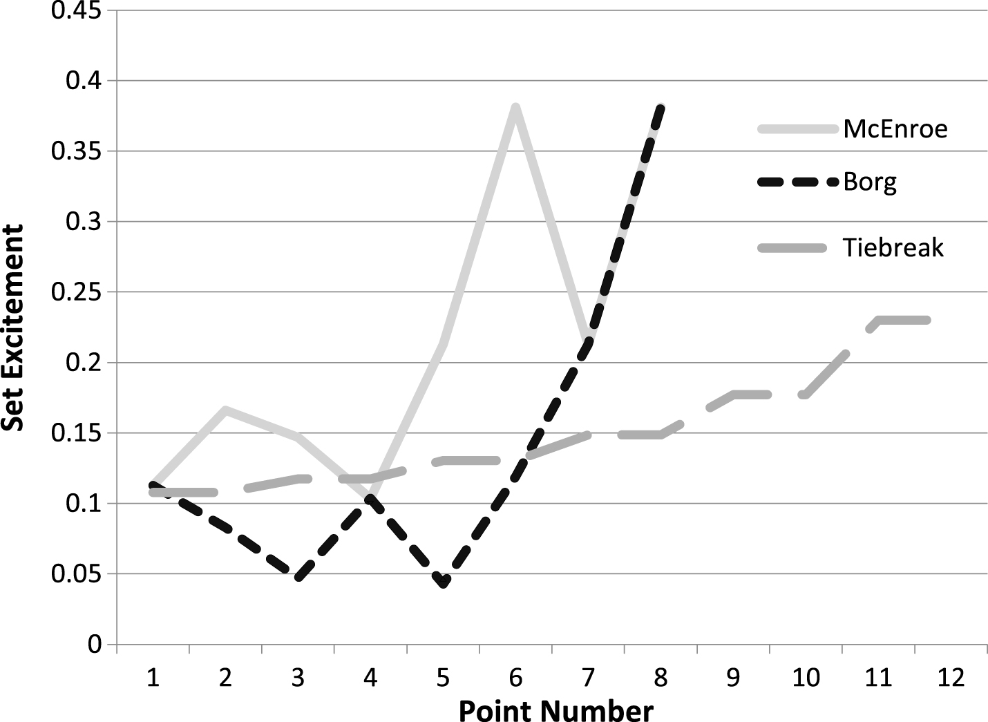
As an example of measuring excitement, we consider the famous 4th tiebreak set between McEnroe and Borg in the final of 1980 Wimbledon. This tiebreak game was won 18-16 by McEnroe. In the 4th set McEnroe won 35 out of 54 points on service, and Borg won 33 out of 52 points on service. Assuming they were equal players on service, the probability either of them would win a point on service can be estimated at 68/106 = 0.6415 for this set. When pa = pb = 0.6415, the tiebreak game has an expected total game-excitement of 1.5292, a variance of 0.6188 and a SD of 0.7867. The observed total game-excitement for this 18-16 result was in fact 6.8817, and this has a standardized-score of 6.8040, clearly a very unlikely outcome, though not as unlikely as a normally distributed score this size would suggest (note: total excitement for the tiebreak game is positively skewed). It is also noted that with these parameters of 0.6415 and 0.6415, which are reasonably typical ones for Wimbledon Men’s singles, the probability that a tiebreak game reaches the score of 16-16 is 0.0005 (or about once every 2000 tiebreak games played). Interestingly, for this 4th set, the observed total set-excitement up to 6-6 (i.e. the observed total game-excitements of the 12 games up to 6-6, weighted by the importances of those games) was 3.3018 compared to an expected value of 3.5592. Thus, the first 12 games of this set had, overall, a slightly less than average total excitement than expected conditional on the set reaching 6-6, even though there were breaks of service in the important 9th and 10th games, and two set (indeed match) points in the 10th game. In the 9th game with McEnroe serving the scores were 0-0, 0–15, 15-15, 30–15, 30-30, 30–40, deuce, AdR, game, and in the 10th game with Borg serving, the scores were 0-0, 15-0, 30-0, 30–15, 40-15, 40-30, deuce, AdR, game. The set-excitements of these points can be seen in Fig. 1. The set-excitements of the points within the tiebreak game can also be seen in Fig. 1. The high level of excitement on the 6th point on McEnroe’s service game and on the 8th point of both their service games can be noted. It can be seen that the tiebreak game was so very exciting because there were so many exciting points. (The point by point outcomes for this match, necessary for the calculation of the observed total excitement for the tiebreak game were located on www.johnwooders.com in one of his research papers (University of Arizona Working Paper 99-05, data). Note that McEnroe served on the first point of the tiebreak game, and the winner of each point was sequentially MBBMMBBMBMBMBMMBMBBMBMBMMBMBMBMBMM, using an obvious notation.)
Fig.1
Point by point set-excitement for the 7th game (McEnroe serving), the 8th game (Borg serving) and the tiebreak game. Note that for the tiebreak game the 11th, 12th, 13th, ... , 34th points all had the same set-excitement measure.
It is clear that for matches in which point-by-point data is standardly recorded and readily available, and this is the case for the more important tennis tournaments, it is reasonably straight forward to carry out the various calculations that have been described above, in a simple routine and automated way. Thus, the summary usually provided for a set could without any particular difficulty include a measure of its total excitement. This objective measure could be used to identify the most exciting set in a tournament, the most exciting set for the year, or even the most exciting set ever played. Note however that for many other characteristics in sport it is simply not possible to make comparisons such as this from one period to another. For example, who is the best tennis player ever?
The method for analyzing excitement outlined above can be used directly for a wide range of scoring systems as used in racquet sports such as table tennis, squash, and badminton, and other sports such as volleyball ... .
2.2Excitement in the situation where the outcome of a ‘unit of play’ includes a draw as well as a win or loss, and applications to other sports such as golf
Example 4. Here we consider the situation in which the outcome of a match can be a win, a draw or a loss to team A with probabilities 0.5, 0.1, and 0.4 respectively. Matches are independent and the competition is the best of three matches, and if the situation is tied after three matches, further matches are played until one team wins a match and thus the competition. The excitement of a particular match (within the competition) is again measured by the expected value of the absolute size of the change in a team’s probability of an overall win as a result of that match being played. In this example we use the notation (x, y) to represent the situation in which y matches have been played and team A is x matches ahead. Note, for example, that there are 3 ways of reaching the state (0, 2), namely WL, DD, LW where W represents a win, D represents a draw, and L represents a loss for team A. Straight-forward ‘backwards’ calculations give the probability values in Table 8, and then ‘forward’ calculations give the excitement values.
Table 8
Values of excitement for the best of 3 matches (with further matches if necessary to break a tie) with each match having win/draw/loss probabilities of 0.5/0.1/0.4
| State | Probability team A wins | Excitement of the state |
| (0, 0) | 0.5822 | 0.2222 |
| (1, 1) | 0.8044 | 0.1991 |
| (0, 1) | 0.5778 | 0.2444 |
| (–1, 1) | 0.3056 | 0.2500 |
| (1, 2) | 0.8222 | 0.2133 |
| (0, 2) | 0.5556 | 0.4444 |
| (–1, 2) | 0.2778 | 0.2778 |
| (0, 3 or more) | 0.5556 | 0.4444 |
Example 5. Match play golf involves 2 players playing against each other. Each golf hole can be won, drawn or lost by player A. The match usually involves playing 18 holes, and if the match is even after 18 holes, further holes are played until one player wins a hole. The excitement of each hole can be determined in a similar manner to Example 4. Table 9 gives results for the 16th, 17th and 18th holes in a match between two equal players whose probabilities of obtaining a birdie, par and bogie on each hole is 0.15, 0.8 and 0.05 respectively.
Table 9
Values of excitement in match play golf between two equal players, each with birdie/par/bogie probabilities of 0.15/0.8/0.05 on each hole
| (Hole, Score) | Probability player A wins | Excitement |
| (19th, 20th, ... , 0) | 0.5 | 0.1675 |
| (18, +1) | 0.9163 | 0.1394 |
| (18, 0) | 0.5 | 0.1675 |
| (18, –1) | 0.0838 | 0.1394 |
| (17, +2) | 0.9860 | 0.0234 |
| (17, +1) | 0.8606 | 0.1208 |
| (17, 0) | 0.5 | 0.1394 |
| (17, –1) | 0.1394 | 0.1208 |
| (17, –2) | 0.0140 | 0.0234 |
| (16, +3) | 0.9977 | 0.0039 |
| (16, +2) | 0.9673 | 0.0358 |
| (16, +1) | 0.8212 | 0.1076 |
| (16, 0) | 0.5 | 0.1208 |
| (16, –1) | 0.1788 | 0.1076 |
| (16, –2) | 0.0327 | 0.0358 |
| (16, –3) | 0.0023 | 0.0039 |
3Discussion
Here we note that the ‘scale’ for the excitement measure in the paper by Vecer et al. (2007) depends on whether the match can result in a draw or not. For illustrative purposes we consider a very simple game consisting of just two points, an a-point (A serves) followed by a b-point (B serves), with pa = 0.9 and pb = 0.4, where pa is equal to the probability player A wins an a-point and pb is equal to the probability player B wins a b-point. This game, denoted by P2 (Play 2 points), can result in a win to player A with probability 0.54, a draw with probability 0.42, or a win by player B with probability 0.04. The possible scores in the game can be represented by (0,0) which is the start, (1,0) where player A wins the first point, (0,1) where player A loses the first point, (1,1) where the players each win a point and the match is a draw, (2,0) where player A wins the match, and (0,2) where player B wins the match. The probability player A wins, the probability player B wins, and the probability of a draw, from each of these particular scores is given in Table 10. It follows that TV(Probability that Player A wins) is equal to 0.54, TV(Probability that Player B wins) is equal to 0.12, and TV(Probability of a draw) is equal to 0.516, giving a total excitement of 1.176.
Table 10
Some characteristics of P2 when pa = 0.9 and pb = 0.4
| Score | P(A wins) | P(Draw) | P(B wins) |
| (0,0) | 0.54 | 0.42 | 0.04 |
| (1,0) | 0.6 | 0.4 | 0 |
| (0,1) | 0 | 0.6 | 0.4 |
| (2,0) | 1 | 0 | 0 |
| (1,1) | 0 | 1 | 0 |
| (0,2) | 0 | 0 | 1 |
Suppose we now consider, for the same two players, the game W2(ALa) which consists of playing pairs of a and b points until one player wins both points, and therefore wins the game. The notation W2(ALa) represents win-by-2 points, whilst alternating a-points and b-points, starting with an a-point. For this game which cannot result in a draw, TV(Probability that Player A wins) is equal to 0.1490 for one pair of points, and TV(Probability that Player B wins) is also equal to 0.1490 for a pair of points. The probability that the first pair of points results in a draw is equal to 0.42, and so the total excitement of the game W2(ALa) which must result in a win to player A or a win to player B can be shown to equal (0.1490*2)/(1 – 0.42) or 0.5137. It is interesting to note that, for these parameter values, this total excitement for W2(ALa) is less than that for game P2 above, even though it amounts to playing an average of 3.4483 points whilst P2 consists of playing just 2 points. It follows that the total excitement for matches which can result in a draw should not be compared with the total excitement of matches that cannot result in a draw. It would appear that the scales for the two systems are different. Also, it is noted that, in the paper by Vecer et al. (2007), the numerical values of the total excitement for matches that can result in a draw were typically larger than those where draws were not possible. This observation is in line with this particular example. However, the differing scales would appear not to be an issue as it would seem that there is never really a need to directly compare a game that can result in a draw with one that cannot.
4Conclusions
Various aspects of excitement in sport have been identified. One aspect has been defined and studied in detail in this paper. This aspect is the excitement that can be attributed entirely to the current score in a match. The excitement of a point played at a specific score is seen to be related to the previously defined ‘importance’ of the point played at that score.
The mathematical definition of excitement is applicable to a wide range of sports scoring systems. Several examples were given, but a major focus of this paper was on a set of tennis. A methodology for determining the average value and variance of the total excitement in the set was outlined. It is reasonably straight forward to use this methodology to determine whether a particular set had a total excitement level that was above or below its expected level, and by how much. This methodology could provide a useful addition to the summary statistics typically provided for a set of tennis. Sets within matches and across matches could be compared objectively for their excitement levels. The most exciting set in a tournament could be determined. The total excitement can be determined even for sets played many years ago, provided the point-by-point data is available. An example of this is the famous and very exciting fourth set in the 1980 Wimbledon Men’s Final between Borg and McEnroe, which has been analysed in this paper.
Examples have also been given where this theory can be applied to the situation in which the outcome at a stage in the match can also be a draw, rather than just a win or a loss as in a point of tennis. One such example is match-play golf.
References
1 | Morris C., (1977) . “The most important points in tennis.” In Optimal Strategies in Sport, edited by Ladany S. P. and Machol R. E., 131–140. Amsterdam: North Holland. (Vol 5 in Studies in Management Science and Systems.) |
2 | Pollard G., (1983) . An analysis of classical and tie-breaker tennis, Australian Journal of Statistics. 25: (4), 496–505. |
3 | Vecer J., Ichiba T., Laudanovic M., (2007) . On Probabilistic Excitement in Sports Games, Journal of Quantitative Analysis in Sports. 3: (3), article 6. |


