
Categorization of crowd-sensing streaming data for contextual characteristic detection
Abstract
The growing reliance on large wireless sensor networks, potentially consisting of hundreds of nodes, to monitor real-world phenomena inevitably results in large, complex datasets that become increasingly difficult to process using traditional methods. The inadvertent inclusion of anomalies in the dataset, resulting from the inherent characteristics of these networks, makes it difficult to isolate interesting events from erroneous measurements. Simultaneously, improvements in data science methods, as well as increased accessibility to powerful computers, lead to these techniques becoming more applicable to everyday data mining problems. In addition to being able to process large amounts of complex streaming data, a wide array of specialized data science methods enables complex analysis not possible using traditional techniques.
Using real-world streaming data gathered by a temperature sensor network consisting of approximately 600 nodes, various data science methods were analyzed for their ability to exploit implicit dependencies embedded in unlabelled data to solve the complex task to identify contextual characteristics. The methods identified during this analysis were included in the construction of a software pipeline. The constructed pipeline reduced the identification of characteristics in the dataset to a trivial task, the application of which led to the detection of various characteristics describing the context in which sensors are deployed.
1.Introduction
In recent years, Wireless Sensor Networks (WSNs) have increased in popularity as a means of monitoring phenomena. Various use cases emerged ranging from smart farms using sensor networks to measuring conditions of the soil [26], to sensor networks deployed in smart cities to control traffic flow [18] or measuring the impact on various environmental factors [2]. Due to the low cost of components, large-scale deployability, and little or no maintenance requirements [8,23], the size of the networks are ever-increasing, resulting in enormous datasets that need to be processed to gain insights. Further, with the increasing ease of use and integration in existing hardware, the number of privately owned sensors is increasing as well. This led to an increase in popularity for crowd-sourced networks [4,6], where various citizens are contributing their privately collected data to city-wide data networks. As the size of these datasets increases, the effort required for extracting insights increases with it, culminating in datasets that require automated methods for processing.
The increasing size of networks raises the risk of misconfigured or faulty sensors impacting data accuracy. This, in turn, influences the conclusions that can be drawn from collected data. With decreasing data quality, erroneous conclusions could be drawn, impacting decisions based on these. To mitigate this, sensor deployment is often standardized to ensure data quality. However, this level of control and expertise is only feasible in networks overseen by a single operator with sufficient resources for monitoring and maintenance. In crowd-sourced networks, this kind of maintenance is not possible. Not only are crowd-sourced networks usually too large to maintain manually, but requiring experts to set up sensors would increase the hurdle for new participants to join and could thereby limit the number of sensors contributing to the network.
Since it is unfeasible to check the deployment configuration of each individual sensor in a decentralized WSN, a software solution is required to process measurements and separate high-quality measurements from low-quality ones. As soon as an incorrectly deployed sensor is detected, the measurements of this sensor need to be ignored when processing the dataset. By comparing measurements from all sensors the same software would be able to extract characteristic deviations within collected data within groups of sensors that share a common context. The presence of such deviations can be expected or unexpected, depending on what is being monitored, possibly requiring observers to take corrective action to avoid a further skewing of measurements [21]. The integration of this kind of software into crowd-sourced networks provides an opportunity to extract additional knowledge from the network, such as exploiting spatial-temporal dependencies between nodes to enrich measurements with insights not available to a single sensory node [8]. These kinds of dependencies are implicitly encoded in the data and can be identified as anomalies if they only affect a single sensor node; or a common deployment context that affects measurements of sensor nodes that might be physically separated from each other but monitoring the same phenomena [12,23].
Due to the large quantity of data that could be present in a crowd-sourced sensor network, an automated process for discovering these context characteristics in time series data is required. In this paper, we introduce a software pipeline that consists of three steps: First, it clusters sensor nodes in a city-wide sensor network based on their collected data. Each cluster describes an unknown context affecting all sensors in this cluster. Second, we generate a simplified model of all collected data by using artificial neural network techniques. We further generate a model for each identified cluster taking only the time series data of this cluster into account. Finally, we compare the created model of each cluster with the general model. This way we can extract cluster-specific characteristics. With these identified characteristics data consumers gain additional knowledge, helping them to identify misconfigured sensors and find common contexts within a crowd-sourced network (e.g., sensors deployed close to roads or parks; cardinal direction of the deployed sensor; sensors that are exposed to direct sunlight at a specific time of the day). Further, with this additional knowledge applications using the collected data, can decide which data should be included or ignored for their given use case. To evaluate our software pipeline we analyzed sensors distributed across Germany and extracted their climate zone as a contextual characteristic.
The remainder of this paper is structured as follows: In Section 2 we will give a short overview of the fundamentals, defining anomalies, events, and preprocessing steps that need to be taken to analyze collected data. The fundamentals are followed by an overview of related work in Section 3, with existing machine learning approaches. Required components for the developed software pipeline are described in Section 4. Finally, in Section 5 we will evaluate our results and conclude this paper in Section 6.
2.Fundamentals
In the following section, we will discuss the fundamentals of various anomalies that can occur within time series data generated by sensors. Each time series contains measurements of a single type (temperature, humidity, e.g.) taken at a specific place at a specific time. Anomalies can range from a single measurement deviating to a whole group of successive measurements that differ strongly from surrounding measurements collected by other sensors. Subsequently, we will define different types of correlation between anomalies, which can lead to interconnected anomalies that we define as characteristics of a group of sensors. Since an isolated anomaly can be classified as an outlier and filtered out, anomalies that occur within measurements of multiple sensors or are repetitive over a given time will most likely be caused by a common context that triggered these anomalies, therefore indicating a characteristic of the common context of affected sensors.
2.1.Anomaly types
To understand how anomaly detection across multiple sensor nodes can benefit the data quality and characteristic detection within a city-wide sensor network, a definition for an anomaly is provided by Grubbs (1969) quoted by Shahid et al. [30, p.195]:
Definition 1.
An outlying observation, or outlier (anomaly), appears to deviate markedly from other members of the sample in which it occurs.
How an outlier or anomaly presents itself in a stream of measurements varies depending on its cause. The simplest type of anomaly within a stream of measurements is a Point Anomaly [7,15]. Point anomaly is an individual data point deviating from the “normal” distribution of values within the data stream as displayed in Fig. 1a. Since these anomalies have no correlation to other data points within the stream, these anomalies are often considered to be noise and should be removed before the data is processed further. As soon as a correlation exists this anomaly is defined as a Collective Anomaly. A collective anomaly can be identified when a collection of related data instances is anomalous concerning the entire data set. In this case, an individual instance of data measured during the anomaly is not anomalous, but their occurrence together as a collection is [7], as can be seen in Fig. 1b.
Fig. 1.
Three different types of anomalies increasing in complexity.
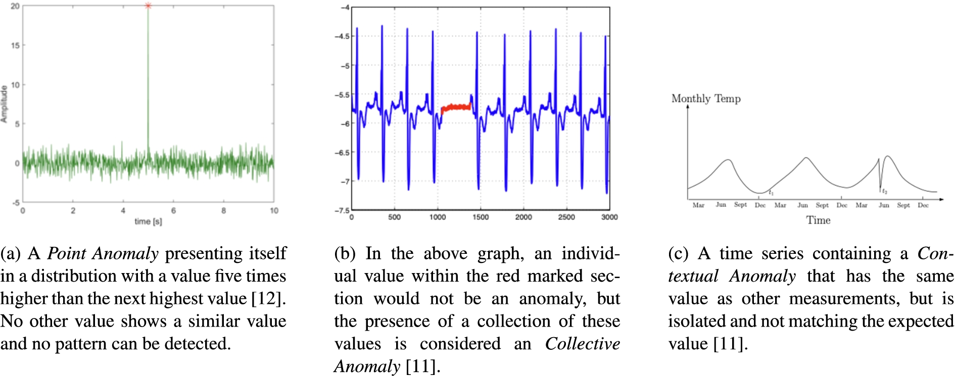
Finally, for some data points, it depends on the context in which they occur to determine if they are anomalous or not. For this reason, these kinds of anomalies are called Contextual Anomalies. When analyzing contextual anomalies, two attributes need to be taken into consideration, namely [7,15]:
1. Contextual attributes, which are used to determine the context for a data instance,
2. Behavioral attributes, which define the non-contextual characteristics of a data instance.
To illustrate how a context anomaly presents itself in a data distribution, consider Fig. 1c. The contextual attribute would be the time scale and the behavioral attribute would be the cosinusoidal fluctuations, defining the “normal” behavior of the temperature during certain times of the year. Using the behavioral attribute values within a specific context allows us to identify a contextual anomaly at
2.2.Correlation of data
While the reason behind an anomaly on a single sensor node is hard to detect, when combining anomalies across multiple sensor nodes anomalies can be grouped and easier analyzed. Therefore a context characteristic can be defined as:
Definition 2.
A context characteristic is a sequence of data anomalies that occurs across multiple data sources over extended periods, allowing us to identify historical patterns [12,30].
Since sensor nodes are distributed within a city-wide sensor network, sensors affected by the same context will have similar anomalies, and therefore a spatial correlation is present between their measurements [8,11,23].
Definition 3.
A spatial correlation exists between nodes in a sensor network when they are deployed spatially dense to each other, resulting in multiple nodes sampling a similar data distribution [23].
Similarly, context characteristics affecting multiple spatially independent sensor nodes, at the same time or in predictable matter encode a temporal correlation in their collected measurements [23]. It is furthermore apparent that measurements collected at one time instant on a single node are related to previous measurements on the same node. Therefore, a temporal correlation can be observed between readings produced by a single or a group of sensor nodes [11].
Definition 4.
A temporal correlation arises when there exists a predictable relationship between sequential measurements on a single or a group of sensor nodes [23].
Understanding the relationship these correlations have with each other, as well as the information contributed by their existence, is imperative and ultimately forms the basis of the approach for detecting contextual characteristics investigated in this paper.
2.3.Time series invariances
Before the similarity between two time series can be measured, it is important to understand which kinds of invariances can occur and what effect these invariances have on the different similarity metrics.
2.3.1.Amplitude invariance
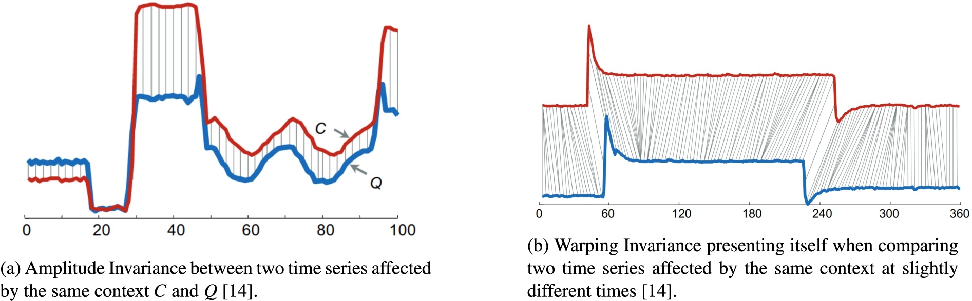
If two sensors are monitoring the same phenomenon, it cannot be assumed that the same values are being measured. Internal differences in sensor configuration or the intensity with which a context affects sensors may result in curves with similar shapes but offset from each other. This kind of invariance is termed Amplitude Invariance [3] and can be identified in Fig. 2a.
Fig. 2.
Two different invariances showing time series data affected by the context.
2.3.2.Warping invariance
Given the continuous nature of context characteristics, such as being exposed to the sun at a given time of day, it is unlikely that sensors affected by these will be influenced at the same time. Often, there is a shift in the time between sensors being affected. These kinds of shifts in the curves are referred to as Warping Invariance [3] and present themselves as seen in Fig. 2b.
2.3.3.Complexity invariances
In addition to considering the shifting of time series, as done in the previous invariances, the complexity of a time series can also influence the effectiveness of a distance metric [3]. An intuitive understanding of the complexity invariances of a time series can be achieved when comparing the number of peaks and values present in the series when calculating the similarity. It has been shown that when complexity invariance is not considered, the distance between a pair of complex time series is often greater than the distance between a pair of simple time series [3] and that complex time series are often found to be more similar to a simple time series than another complex time series [3]. While the effect of complexity invariance can be somewhat mitigated by using an approach that corrects for warping invariance [3], it is advantageous to not only rely on these methods.
2.3.4.Multiple invariance
It is also possible that two time series might differ because of a combination of the invariances mentioned above. This will most often be the case since each node in a sensor network will have its own sensor, thereby introducing potential amplitude invariance. And, while the nodes might be sampling the same distribution, nodes will not be deployed in the exact same physical location, thereby introducing potential warping invariance. The complexity of time series can also differ easily, even in the case where nodes have the same hardware and are running the same software. Communication problems can result in missing values that need to be considered when computing the similarity. The metric that we choose to describe the similarity between time series, therefore, needs to address these invariances.
3.Related work
When attempting to detect anomalies in time series, most approaches can be categorized as belonging to one of two groups: either an anomaly is identified as discrepancies from a model of expected values, or time series are analyzed for containing patterns learned from models of a known anomaly [13]. The first category has the advantage of being able to identify unknown kinds of anomalies that might represent unknown contextual characteristics. If measurements deviate far enough from the expectation these measurements are considered a series of anomalies. If a series of anomalies is detected within a group of sensors it is classified as a new unlabeled characteristic. For accurately detecting already known characteristics, the second group of approaches is more suited but needs existing models representing the series of anomalies that represent this characteristic. To be able to detect multiple characteristics, multiple models are required, which increases the complexity of the detection process.
3.1.Predictive models
Predictive models for anomaly detection belong to the first category introduced above and rely on the usage of previous observations to anticipate future values a sensor node will produce [7]. Any new, unseen data is compared to the predicted value from the model to determine to which class it belongs. If the measured value is similar to the predicted value, the input is accepted as normal. However, if the actual value differs too much from the predicted value, it would be classified as an anomaly [7,15]. If multiple, subsequent anomalies are observed, they can then be classified as a characteristic.
3.2.Autoencoders
A common method used for generating a model of a time series is the use of autoencoders [14,25]. Autoencoders are specialized neural network topologies that are trained in an attempt to copy their input to their output [14]. Due to this unique characteristic, autoencoders are often referred to as semi-supervised learning methods since they partially rely on techniques that are more commonly found in supervised learning. Consisting of an input layer, 1 to n hidden layers, and an output layer, an autoencoder can be divided into an encoder function
3.3.Support vector machines
Another model-based approach for anomaly detection in time series has been developed based on the usage of Support Vector Machines (SVMs), specifically in the form of one-class SVMs [35]. This approach utilizes the excellent generalization provided by SVM-based models and extends it using a specialized kernel. The usage of this kernel improves the performance of identifying anomalous time series [7]. Given that SVM is a supervised method, labeled data is required for training these kinds of models.
3.4.Deep temporal clustering
Deep Temporal Clustering was developed to extract informative features on various time scales, which makes it ideal for handling longer data sequences [22]. This is achieved by using a specialized temporal autoencoder, which can achieve greater dimensionality reduction by collapsing input sequences in all dimensions except temporal [22]. Once the dimensions have been reduced, the internally encoded sequence is fed into the clustering layer.
The novel temporal clustering layer, which is built specifically to handle unlabeled spatial-temporal data [22], was agnostic of the similarity metric that is used for the actual clustering. This makes the framework flexible to apply to data gathered from various domains by using a similarity metric that is best suited for the data. Furthermore, this allows simplified prototyping with different metrics to determine which of them form the most meaningful clusters.
3.5.Swift event
SwiftEvent [13] is an anomaly detection algorithm that falls into the second of the categories described previously. Relying on labeled data, SwiftEvent learns the characteristics of a specific, user-defined anomaly using supervised learning methods. Once the detection of these anomalies has been learned, the model can be applied to real-time data to detect the occurrence of learned anomalies. Training of the models is achieved by projecting marked anomalies into a representation befitting the features. Similar anomalies will have similar projected representations, forming clusters. For each of the formed clusters, a model will be trained, which can then be used for detecting the presence of the characteristic.
4.Constructing a pipeline
In this chapter, a software pipeline will be created utilizing previously presented techniques. This pipeline enables a city-wide sensor network to classify its sensors based on their collected data. For this purpose, each step is described that the pipeline must fulfill to be able to cluster sensors based on their contextual characteristics. Input for this pipeline will be time series data from a large set of sensors measuring a specified type of data. The developed pipeline outputs a categorization of the sensors and their data into different categories, which themselves are not labeled. Rather, the differences between the clusters will be highlighted, so that in an additional manual step it can be determined which context affects sensors in these clusters.
4.1.Similarity metrices
When performing any sort of clustering on data, it is important to choose an appropriate similarity measure to ensure the formation of logical clusters. In the case of time series data, choosing a similarity metric is not as simple as, for example, when working with geometric distances. As discussed in Section 2.3 different invariances influence the distance between two time series affected by the same real-world phenomena. To measure the similarity between two time series data streams different approaches exist that take different invariances into account. Most common distance metrics are lock-step measures such as the Euclidean Distance [10], while others use elastic measures such as Dynamic Time Warping [5].
4.1.1.Euclidean distance
The most common distance metric that is used for clustering is the Euclidean Distance [17]. Due to its simple implementation, it is often the first metric to be considered when forming clusters.
The Euclidean Distance requires two time series Q and C of the same length n,
Euclidean Distance therefore compares all measurements at the same index, this makes it vulnerable to all invariances. When considering time series data from deployed sensor nodes potential differences in sensor configuration and placement lead to curves that have no invariances.
4.1.2.Dynamic time warping
One solution to take invariances into account is Dynamic Time Warping (DTW). DTW is a method used on time-dependent data to find an optimal alignment between two time-dependent sequences [3,9,32]. Often used in the field of speech recognition, this method has been successful at matching similar speech patterns spoken at different tempos [9].
Fig. 3.
A comparison of using Euclidean distance (left) and DTW (right) to measure similarity between time series [36].
![A comparison of using Euclidean distance (left) and DTW (right) to measure similarity between time series [36].](https://content.iospress.com:443/media/scs/2023/2-2/scs-2-2-scs230013/scs-2-scs230013-g003.jpg)
When considering Fig. 3 a comparison between using a lock-step distance such as the Euclidean Distance to determine the similarity between time series data (left) and using DTW (right) can be seen. In causal relationships, there is often a lag in a phenomenon’s presentation to individual observers. As an illustrative example, consider multiple nodes of a sensor network deployed densely together but in cardinal directions of a building monitoring temperature. While sensors deployed east of the building would measure higher temperatures in the morning and lower temperatures in the evening. The opposite happens with sensors deployed west. While sensors deployed south have higher temperatures nearly consistently. Despite this, the same characteristic would be observed by all the affected nodes and should therefore be clustered together. If the Euclidean Distance were to be used when comparing time series, data points measured at the same time would be compared. Therefore, it is necessary to use a metric that is impervious to this effect when comparing time series. DTW is an attempt to consider the warping invariance of the data when calculating the similarity.
Formally DTW can be defined as an optimization problem. Given two time series
While the alignment of peaks and valleys also indirectly improves dissimilarities introduced by complexity invariance, this method does not account for the varying number of peaks and valleys which might be present in the series and will therefore potentially not be able to find the best alignment.
One of the main disadvantages of DTW is the quadratic time and space requirements of the algorithm [29]. This limits the cases in which it can be used to those with a relatively small number of time series data since it would otherwise become infeasible to use this algorithm. An optimized implementation of DTW, called FastDTW [29], was therefore developed, which has a linear time and space requirement, thereby greatly increasing the cases in which this metric can be used.
4.2.Clusters in a dataset
After examining methods to determine the similarity of time series data, we need to cluster time series data sources based on the similarity in their collected data. Since the number of distinguishable characteristics is unknown, the number of clusters needs to be found. Therefore, a method of empirically determining the number of clusters that could be present in the data needs to be defined. In the following, two heuristic methods that are commonly used when no additional knowledge is available concerning the number of clusters in a dataset will be introduced.
4.2.1.The elbow method
One of the most commonly used methods is the Elbow Method. This method works by iteratively increasing the number of clusters to be formed and examining the effect the formation of additional clusters has on the inertia.
Definition 5.
Inertia is the sum of squared distances of samples to their nearest cluster center, also known as an intra-cluster variance.
Fig. 4.
An example of an elbow graph with the optimal value for k marked in red.
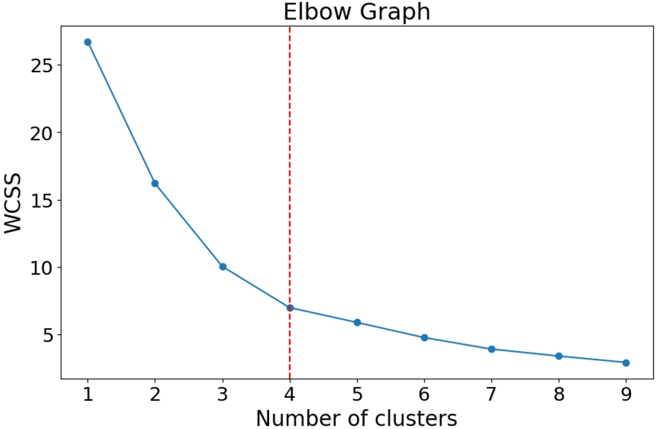
Initially, an increase in the number of clusters will have a significant effect on the intra-cluster variance. If this were not the case, it would indicate that the data could not be divided into multiple clusters and would signal the end of the analyses. However, as the number of clusters increases, a point is reached after which the effect on the inertia is drastically reduced, visually resulting in an elbow when plotted. This effect is a result of the clustering algorithm not being able to decide to which cluster a sample should belong and is therefore an indication that too many clusters have been formed. Since there is no greater reduction in the inertia after a certain number of clusters, increasing the number of clusters offers no advantage. This number of clusters, after which the inertia decreases linearly when adding more clusters, will be taken as the optimum number. To demonstrate what such an elbow curve might look like, consider the curve formed when clustering an example dataset, as can be seen in Fig. 4.
From Fig. 4, it is clear to notice that after three clusters have been formed, additional clusters have less influence on the variance. This is an indication, therefore, that the model is overfitted for the data and meaningful clusters are no longer being formed, but instead, the data is split more randomly.
4.2.2.Silhouette score
Another heuristic that is commonly used for determining the correctness of formed clusters is to calculate the so-called Silhouette Score [28]. This score measures the inter- and intra-cluster variation to determine the effectiveness of formed clusters. In a similar fashion to the Elbow Method mentioned previously, determining the Silhouette Score relies on iteratively increasing the number of clusters into which the data should be divided. After each iteration, the Silhouette Score is then calculated for each of the samples assigned to a cluster.
After data has been assigned to their respective clusters, two measures need to be calculated before being able to determine the Silhouette Score. For a sample i assigned to cluster A, determine
A great advantage of the Silhouette score is its simple interpretation. A calculated score of 1 indicates a well-formed cluster. For a particular sample i where
4.3.Clustering of time series data
To identify contextual characteristics we first need to identify sensors deployed in a similar context. To do so, sensors are clustered based on the similarity of their collected data. Each cluster contains all sensors that are placed in a similar context and therefore, show similar characteristics in their collected data. Following different algorithms are introduced to find the most expressive clusters.
4.3.1.K-means clustering
The K-means clustering algorithm is possibly the most well-known method in the partitional clustering category.
Definition 6.
In Partitional Clustering, clusters are characterized by a central vector, and data points that are close to these vectors are assigned to the respective clusters.
This method attempts to minimize the intra-cluster variance while simultaneously maximizing the inter-cluster variance [1,34]. This leads to maximally dense clusters (i.e., the points in a cluster are maximally similar) while clusters are maximally separated from each other by some distance metric. Formally, this optimization can be expressed as:
Definition 7.
Given a set of d-dimensional observations
This method works by randomly partitioning objects into nonempty subsets and constantly adding new objects and adjusting the centroids. These steps are repeated until a local minimum is met by optimizing the sum of the squared distance between each object and the centroid [34]. Even though K-means is an unsupervised method, there are still hyperparameters that need to be determined for each application, such as a predetermined k for the number of clusters that are to be populated [34]. Therefore, this clustering needs to be repeated and the correct number of clusters needs to be determined using methods from Section 4.2.
Traditionally, the Euclidean distance is used to determine to which cluster a data point belongs. This metric is, however, unsuitable as a distance metric for time series data since the time dimension is ignored, resulting in shifted time series having a large Euclidean distance and therefore not belonging to the same cluster. Furthermore, it has been demonstrated that applying traditional clustering methods, such as K-means, directly to spatial-temporal data usually results in severe overfitting and poor performance [22].
4.3.2.Density peaks
Density Peaks is the most popular in its class of density-based clustering algorithms for time series data [19]. These kinds of methods allow for the construction of non-spherical clusters, which is not possible in partitional clustering methods, such as K-means [27].
Definition 8.
Density-based Clustering considers the density of data points when forming clusters instead of distances. Therefore, cluster centers are defined to be the densest region in a data space [27].
Cluster centers are determined by calculating the local density
After identifying the cluster centers as the points with the highest local density, neighboring points are assigned to clusters based on the neighborhood distance
Other than K-Means, DP does not rely on the number of clusters as an input parameter. Since the given parameters define what would be considered a meaningful cluster, this method can independently determine the number of clusters to form from the given parameters. This is advantageous in cases where the number of clusters in the data is unknown but the idea of what should be considered to be a meaningful cluster is. Finding the correct parameters for DP therefore also relies on domain knowledge and empirical evidence. Since in this paper domain knowledge is not taken into account to make it applicable for different use cases this method is not applicable.
4.3.3.Deep temporal clustering
As described in Section 3 Deep Temporal Clustering is an architecture that combines well-known neural network methods with a novel temporal clustering layer, thereby forming a single end-to-end learning framework [22]. This unsupervised learning method makes use of an autoencoder topology in combination with Long-Short Term Memory (LSTM) and convolutional layers to reduce the dimensionality of the input data and cluster the reduced data [22].
4.4.Model generation using artificial neural networks
With the created clusters, sensors deployed in a similar context are now grouped. To highlight characteristics that define these clusters we utilize artificial neural networks (ANN) by generating an abstraction model for each cluster. This model will then be compared to a generated model based on all sensors, showing the main differences and therefore the meaningful characteristics of this cluster.
4.4.1.Artificial neural network
ANNs are inspired by our brains, consisting of neurons communicating with each other over a network of electrochemical activity. These kinds of networks attempt to emulate our understanding of how the brain works by copying its structure and communication methods to form networks that can be trained to solve complex problems. Similar to the neuron being the most basic unit in the brain, a mathematical model of a neuron (called a perceptron) is the most basic unit in an ANN.
Definition 9.
A Neural Network is a computational model consisting of a network of simple mathematical functions called “neurons” [14]. The properties of such a network are determined by its topology and the properties of the neurons it consists of [31].
In feed-forward neural networks information flow in one direction. If the neurons in such a network consist of simple perceptrons, which cannot build up a memory of previous inputs, it can be expected that they will not perform well on time series data, where temporal dependencies are present and crucial to consider. To address this problem, various adaptations of the network are possible.
4.4.2.Long-short term memory
When working with time series it is important to take the past into account generating a more general model of a set of given timer series data. LSTM cells are an example of artificial cells that are specialized in processing longer sequences of input. Instead of a simple feed-forward activation function, as is present in the perceptron, LSTM cells have an internal recurrence that produces paths where the gradient can flow for long durations, thereby mitigating the vanishing and exploding gradient problems present in RNNs [14,16]. The so-called “LSTM cell” enables networks to learn long-term dependencies more easily by incorporating gates that control the weights being fed into the network [14,16].
4.4.3.Autoencoders
Autoencoders are semi-supervised neural networks that can learn the patterns of multiple time series and can be used to identify deviations [14,25]. Autoencoders of particular interest for this investigation are the so-called undercomplete autoencoders [14]. This kind of network has the unique characteristic that the hidden layer has a lower dimensionality than the input and output layers, forming a bottleneck. During the training process, input data is compressed down into ever-shrinking hidden layers, thereby constructing an internal representation from which the output is reconstructed by expanding the internal representation back to the input dimensionality. The model is thereby forced to prioritize input data and, in so doing, isolate the important properties [14]. As a result of this network topology, anomalies are not present in the internal representation, as they do not conform to the general observed distribution. The success of the training is then measured by calculating the loss between the reconstructed output and the initial input. During this phase, anomalies can be identified since they would not be present in the reconstructed internal representation.
Due to the prioritization of input features, a certain loss is to be expected in the reconstructed model. The training process can be described as minimizing this loss:
Should the produced model match the input data exactly, we can speak of the model overfitting the input.
Definition 10.
Overfitting is “the production of an analysis that corresponds too closely or exactly to a particular set of data, and may therefore fail to fit additional data or predict future observations reliably” [24].
An overfitted model has been over-specialized to describe the training data set and will therefore not generalize well for new data that were not part of the training set.
5.Evaluation
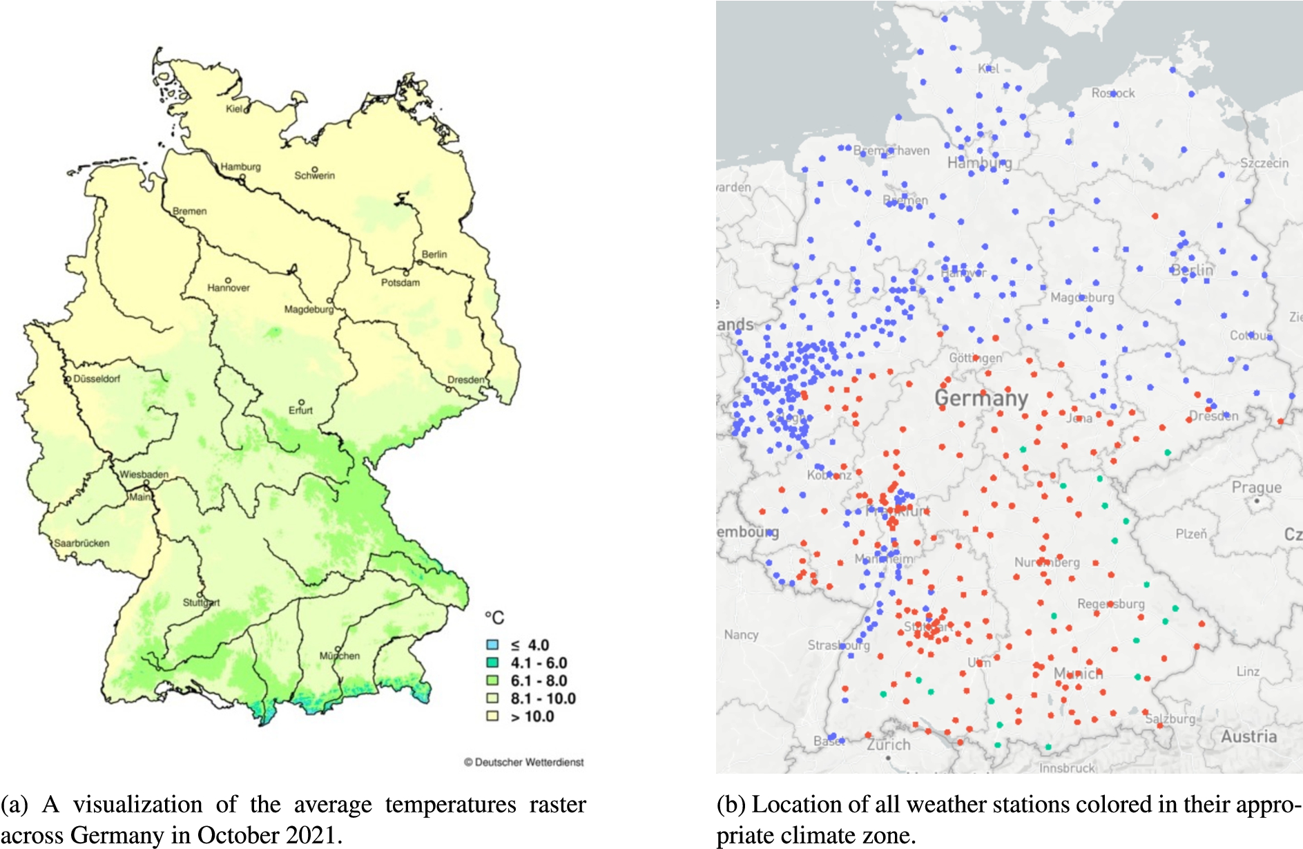
While we identified multiple methods that can be useful for exploiting encoded spatial-temporal dependencies in time series data to extract contextual characteristics from deployed sensors, this section will investigate their effectiveness by analyzing real-world data. To evaluate different methods and compare their effectiveness sensor data was generated by approximately 600 weather stations spread across Germany. These weather stations are deployed in a standardized manner, resulting in fewer contextual characteristics encoded in the sensors. One of the remaining characteristics is the corresponding climate zones in which the sensors are deployed. This classification is also provided by Deutscher Wetterdienst (DWD), the German weather and climate authority, which allows us to control the correct classification.
5.1.Dataset
To effectively evaluate the exploitation of spatial and temporal dependencies, a dataset of time series containing such dependencies is required. The physical separation between nodes encodes the spatial dependencies, while the concurrent observation of the same phenomenon is responsible for introducing the temporal dependencies.
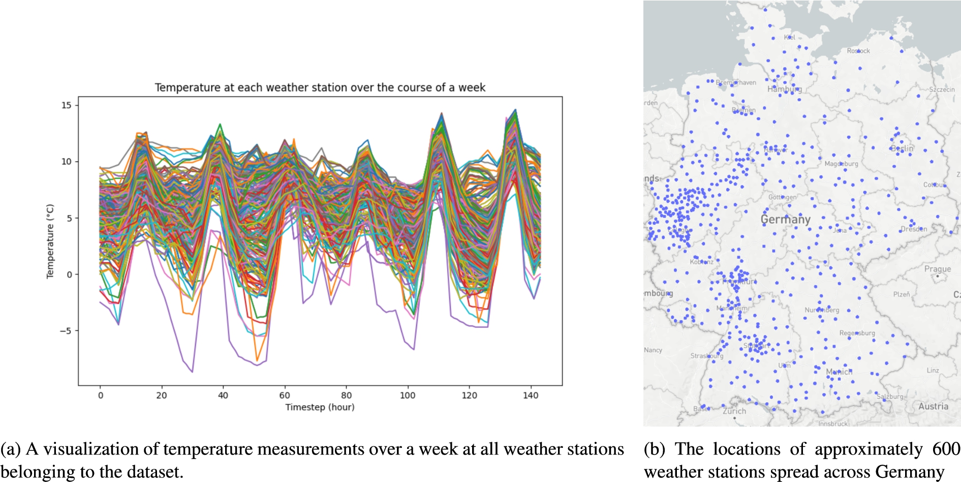
Data gathered by approximately 600 weather stations spread across Germany, the locations of which can be seen in Fig. 5b, was accumulated to construct a dataset that is large enough to better determine the effectiveness of various stages of the proposed approach. The resulting 600 time series contained in the dataset consists of the average temperature measured at the location over a week. The wide geographic spread of the sensors covers many different environments, which leads to varying measurements in the dataset. This poses the ideal circumstances for analyzing the usefulness of the approach. Going through the data of each station would be time-consuming and tedious. However, automating this task could result in discovering interesting characteristics that could easily be missed otherwise.
Figure 5a visualizes the measurements from all weather stations over a week. It would be a laborious task to extract possible contextual characteristics that could be present from this overwhelming graph, not to mention the possibility of mistakes due to the human factor. This is the main motivation for investigating modern approaches to extracting this information in an automated fashion.
Fig. 5.
Data set of approximately 600 weather stations deployed in Germany. Average temperature within a week.
5.2.Outlier removal
In Definition 1, anomalies are defined as being sparse in the data and not conforming to the usual pattern of the data in which they are found. Anomalies affecting only a single sensor are unnecessary information and usually are the result of sensor or network errors. These kinds of anomalies should be removed before constructing a generic model since they could negatively influence the accuracy of clustering and models that will be trained based on the data. However, it would be a mistake to attempt to remove all anomalies. Definition 2 describes contextual characteristics as consisting of a series of anomalies. It would therefore be unfortunate if contextual characteristics were removed during the process of outlier removal. In the following section, the removal of point anomalies, which were introduced in Section 2.1, will be analyzed using Principal Component Analysis (PCA) [14]. In the following, the effectiveness of this method will be analyzed when applied to the dataset.
While more than 40 principal components were found contributing to the variance in the dataset, with each principal component the contribution got significantly smaller. From the results summary shown in Table 1, it can be seen that the initial dimensionality of the input dataset
Due to the dataset being produced by a third party, it is unknown if the data has been processed in any way before. For this reason, outlier removal will be applied rather conservatively by opting for the removal of only 0.1% of the variance. When working with raw sensor data, the degree of outlier removal will probably be much greater. The dataset resulting from the above process will be used for the remainder of the investigation.
Table 1
The percentage of variance which is described by an increasing number of components
| Number of components | Explained variance (%) |
| 2 | 80 |
| 4 | 90 |
| 20 | 99 |
| 39 | 99.9 |
5.3.Comparing different clustering methods
To accurately validate the performance of clustering methods, the correct clusters to which each sample should belong must be known. However, since the data is unlabelled and, therefore, the exact configuration or context in which each station is deployed is unknown, a proxy ground truth is required to perform the evaluation. One such substitute, in this case, is the use of the different climate zones across Germany to identify potential clusters that are expected to form. The climate of each region is influenced by various factors, including elevation and proximity to large bodies of water. It can therefore be expected that measurements taken from regions with similar climates should be clustered together since nodes from the same region will be sampling similar distributions, and therefore the distances between the time series should be small. A raster grid aids in the mapping of average temperature measurements across the country over a month to define the expected clusters.
Fig. 6.
Reference data provided by the DWD, shows that weather stations should be divided into three climate zones.
The raster grid is made available in the ESRI ASCII Grid format at a resolution of
In the following, the performance of the clustering methods discussed in Section 4 will be compared. By performing the clustering based on the various similarity measures mentioned in the same section, the ability of each method to form the expected clusters shown in Fig. 6b will be compared. To better compare the different similarity measures that were proposed, the evaluation will be split into two tables. In Table 2 the Euclidean Distance will be used as a similarity measure, while Dynamic Time Warping (DTW) will be used in Table 3. Using each of these similarity measures, the three clustering methods will be evaluated. For each of the methods, the clustering process will be applied multiple times, selecting the best-performing iteration of each method for comparison.
Table 2
The performance of different clustering methods with Euclidean distance as the similarity measurements
| Precision | Recall | Rand Index | F1-Score | MCC | |
| K-Means | 0.76 | 0.65 | 0.73 | 0.71 | 0.47 |
| DPC | 0.71 | 0.78 | 0.73 | 0.74 | 0.46 |
| DTC | 0.73 | 0.83 | 0.76 | 0.78 | 0.54 |
Table 3
The performance of different clustering methods with dynamic time warping (DTW) as the similarity measure
| Precision | Recall | Rand Index | F1-Score | MCC | |
| K-Means | 0.75 | 0.77 | 0.76 | 0.76 | 0.52 |
| DPC | 0.73 | 0.77 | 0.75 | 0.75 | 0.49 |
| DTC | 0.80 | 0.62 | 0.74 | 0.70 | 0.48 |
In general, when comparing Tables 2 and 3, it is clear that the clustering methods performed fairly equally. During the sole consideration of Table 2, where the Euclidean Distance is utilized as a distance metric, Deep Temporal Clustering (DTC) outperformed the other contenders on clustering the dataset in almost all metrics and is, therefore, the only candidate that comes into consideration. However, when including Table 3 to the consideration, where Dynamic Time Warping is used as a metric, a reduction in the performance of DTC can be noticed. In comparison, the performance of Density Peak Clustering (DPC) and K-Means has improved and is comparable to the results achieved by DTC using the Euclidean Distance as the distance metric. Table 4 summarises the comparison between the remaining candidates:
Table 4
A side-by-side comparison of the performance of the best clustering candidates, irrespective of distance metric
| Precision | Recall | Rand Index | F1-Score | MCC | |
| K-Means (DTW) | 0.75 | 0.77 | 0.76 | 0.76 | 0.52 |
| DPC (DTW) | 0.73 | 0.77 | 0.75 | 0.75 | 0.49 |
| DTC (eucl) | 0.73 | 0.83 | 0.76 | 0.78 | 0.54 |
As can be seen in Table 4, although the achieved results are very similar, DPC performed slightly worse and is therefore eliminated as a candidate, leaving DTC and K-Means as the remaining options. During the evaluation of these remaining candidates, it was noticed that DPC had much higher computational requirements than K-Means while producing very similar results. Since the dataset in this investigation consists of univariate time series, the unnecessarily complex processing done by DTC becomes a burden to itself. In future iterations of this process, where multivariate time series might be investigated, DTC should be reevaluated as a possible clustering candidate. Furthermore, from the research done in Section 4, DTW is currently the state of the art when it comes to time series comparison and would therefore potentially apply to more kinds of time series than using the Euclidean Distance. For these given reasons, K-Means was selected to be the clustering method to be used for the remainder of the investigation.
5.4.Cluster analysis
In the previous section, the predefined three climate zone were used as the “correct” number of clusters present in the data. This was a best-guess assumption, which enabled the analysis of the performance of various clustering algorithms. It is, however, not necessarily the correct number of clusters. In the following, the heuristics discussed in Section 4.2 will be applied in an attempt to find the correct number of clusters. Figure 7a displays the Elbow Curve created by clustering with K-Means with a number from one to nine clusters.
To identify the correct number of clusters using this method, as described in Section 4.2.1, three clusters are identified as the number of clusters that are present according to this method. From Fig. 7a it can be seen that forming more than three clusters results in a linear reduction in the variance for each additional cluster being added. This is an indication of overfitting taking place.
To support the finding of the Elbow Curve, the Silhouette Score is calculated as a comparison based on the same dataset. Having understood what is expressed by the Silhouette Score in Section 4.2.2, the score can be calculated for an increasing number of clusters in our data, similarly to how the Elbow curve was obtained. Since it would be impractical to show the scores of all samples in all clusters to make a decision, instead the mean Silhouette score over all samples will be calculated, as can be seen in Fig. 7b.
Fig. 7.
Comparing both methods, three clusters are selected as the optimal number of clusters.
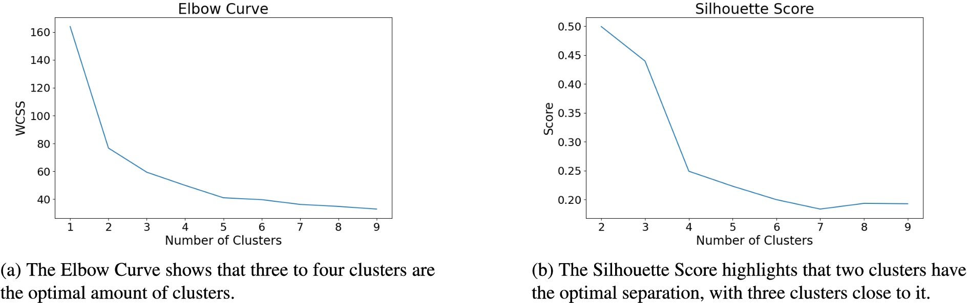
Figure 7b shows a decreasing mean Silhouette Score as more clusters are added. The highest score is achieved when two clusters are formed. Even though the Silhouette Score suggests two clusters for optimal separation between clusters, the score for three clusters is not much lower. In addition to the Elbow method finding three to be the most suitable number of clusters, as well as this being the number of clusters naively found in Section 5.3, forming three clusters would allow for more interesting analyses to be done. For these reasons, three will be used as the number of clusters for the remainder of this work.
5.5.Autoencoder
Based on the various architecture components described in Section 4.4.3, an autoencoder based on LSTM cells can be constructed which can learn a generic model based on the input time series. A generic model allows for the summarisation of multiple time series into one, which simplifies the comparison between the time series belonging to a cluster. Since the cluster from which the autoencoder will be formed consists of multiple time series, any sequence of anomalies (or contextual characteristics) that occur in multiple time series will be encoded into the generic model. This functions as a filter, removing contextual characteristics that are unique to a single time series, as well as including contextual characteristics that are present in multiples. A description of the various layers can be seen below:
Model: "autoencoder"
_________________________________________________________________
Layer (type)                Output Shape              Param #
=================================================================
input_2 (InputLayer)        [(None, 3, 163)]          0
input_layer (LSTM)          (None, 3, 144)            177408
hidden1 (LSTM)              (None, 3, 32)             22656
hidden2 (LSTM)              (None, 1)                 136
bridge (RepeatVector)       (None, 3, 1)              0
hidden3 (LSTM)              (None, 3, 1)              12
hidden4 (LSTM)              (None, 3, 32)             4352
hidden5 (LSTM)              (None, 3, 144)            101952
time_distributed_1 (TimeDis  (None, 3, 163)           23635
tributed)

=================================================================
When the above-listed layers are compared to the generic architecture presented by [22], clear similarities are apparent. The input is compressed into more complex embedded representations as it flows through the network. Once the training has been completed, a lower-dimensional model has been trained, which can be used as a generic model for all the data that was input into the autoencoder. To illustrate the generalization produced by the application of an autoencoder, the dataset was used to construct a generic model of all weather stations across Germany.
In Fig. 8 the performance of the autoencoder training can be seen. The first graph shows the measurements of all weather stations for a week. This is the input to the autoencoder and what will ultimately be compressed. The second graph is the generic model that was constructed using the autoencoder. The keen reader would have seen that the temperature measurements have been scaled. The main focus of the investigation is to determine discrepancies between the patterns of cluster models. To determine this, the actual values are irrelevant and have therefore been normalized. Additionally, normalizing the values in the time series mitigates the effects of amplitude invariance.
Fig. 8.
The training process for a generic model of all data in the dataset.
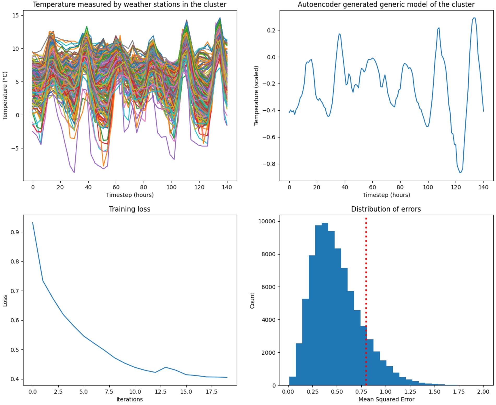
Visually determining the performance of the autoencoder is not simple, therefore two further graphs were added to aid in the evaluation. The next graph shows the performance of the loss during each iteration of the training process. This gives us an idea of whether the training was successful, how much loss is present in the generated mode, and helps determine the number of iterations necessary to train a well-performing model. To avoid overfitting the model to the data, it is essential to stop the training process before overfitting occurs. When considering the graph, a point can be identified where the rate at which the loss is decreasing becomes almost linear. This is an indication of the model starting to overfit the data, and training should therefore be stopped. Additionally, a second graph visualizes the distribution of the loss over the input. This distribution helps decide the threshold after which a sample would be considered an anomaly. Since anomalies are sparse and not present in multiple time series, they will not be present in the generic model of the cluster. They can therefore simply be identified as the samples that have a large loss when compared to the generic model. As an example, a red line was added to the loss distribution graph as an indication of a possible threshold. In this example, all samples that have an error larger than 0.8 will be identified as anomalies.
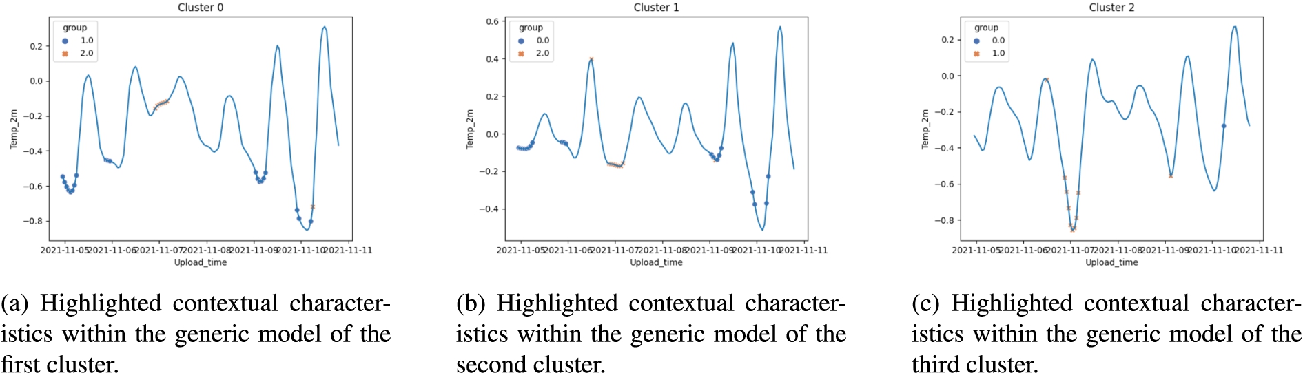
5.6.Identifying contextual characteristics
Having now identified the best methods to cluster and create generic models of the time series, these methods can be applied to forming three generic models, one for each of the clusters formed using K-Means with DTW as the similarity metric. Using the generated models, the focus can be shifted to identifying contextual characteristics. Since each of the cluster models was generated based on multiple time series belonging to the cluster, the models have therefore encoded contextual characteristics which are present in multiple time series. The identification of contextual characteristics has thus become trivial due to the time scale being correlated across all clusters. By comparing the models of each cluster with each other, discrepancies can be identified.
Similar to what has been done in previous steps, when performing the identification of the contextual characteristics, it is necessary to determine an “error threshold” after which a sequence should be considered to be a contextual characteristic. This will likely be different depending on the use case and must be determined empirically. If a very large threshold is chosen, no contextual characteristics will be identified. Conversely, if a threshold is chosen that is too low, every time step will be considered an anomaly or belong to a contextual characteristic. In the case of our dataset, a threshold of 0.4 was determined and used. Any difference between the generic models larger than 0.4 will therefore be considered to be anomalous and belong to a contextual characteristic. The contextual characteristics identified between the clusters in the dataset are visualized with markers in Fig. 9. When calculating the difference between the models, it is unknown which of the models being compared is the source of the contextual characteristic. The automatic detection of this might be analyzed in a future iteration. Therefore, the contextual characteristic is marked in both models. As an additional advantage, the marking of corresponding contextual characteristics simplifies the comparison between the models since the graph of a single model contains information from others. This approach, however, doesn’t scale well and could become problematic should many clusters be present in the data.
Several anomalies (or contextual characteristics) could be identified, as shown in Fig. 9. All contextual characteristics were recognized due to a discrepancy larger than 0.4 between the cluster graphs. When only considering the discrepancies between Figs 9a and 9b, it can be deduced that during four periods in the week, the difference between Fig. 9a and 9b was large enough to be considered anomalous. When comparing Fig. 9c to the other two clusters, a clear anomalous event can be seen. During one period, the temperatures of nodes in cluster two behaved very differently than the temperatures in the other clusters.
Fig. 9.
Contextual characteristics discovered in each of the clusters.
6.Conclusion
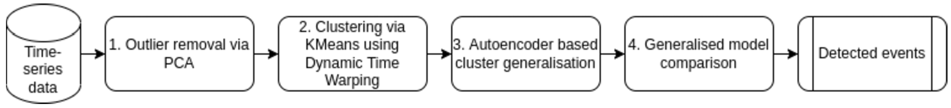
In this paper, we analyzed various methods applicable in different steps of detecting contextual characteristics based on spatial-temporal dependencies in time series. As a result, a pipeline can be constructed consisting of the steps identified during this investigation, as depicted in Fig. 10. Once a time series dataset has been collected containing data with spatial-temporal dependencies, such as data collected by a wireless sensor network, PCA is applied to the data to remove point anomalies (1). This preprocessing step improves the performance of the clustering step that follows. K-Means clustering based on Dynamic Time Warping as a similarity measure was shown to form the best clusters and should therefore be applied once the anomalies have been removed (2). The third step exploits the spatial dependencies in the data due to the assumption that sensors deployed in similar contexts will be clustered together since they are sampling from a similar distribution. Once the clusters have been formed, they can be generalized using an autoencoder in step four. Since contextual characteristics would have affected multiple sensor nodes in that region at about the same time, the characteristic will be encoded into the generalization for that region’s cluster. Generalized models are based on samples taken during the same period, therefore, discovering characteristics in the clusters results in comparing the correlating measurements encoded in the models and returning the identified characteristics as a result.
Fig. 10.
A flow diagram showing the necessary steps identified to detect contextual characteristics based on spatial-temporal dependencies.
Our Evaluation showed, that we can detect an expressive number of clusters within a large number of time series data. By analyzing these clusters we can identify multiple characteristics within each cluster that separates it from other. While we used temperature data within our evaluation, we believe that this can be easily applied to different contextual data, since we did not add any context information, that is specific to temporal data. Using this information we want to focus on learning which contextual influence led to these characteristics, to conclude the deployment of sensors. Further, we want to analyze how many characteristics can be identified within a smart city context with a much denser sensor distribution. One interesting use case we focus on is the detection of Urban Heat Islands [20], which would allow us to warn affected citizens.
Conflict of interest
None to report.
References
[1] | M. Abu Alsheikh, S. Lin, D. Niyato and H.P. Tan, Machine learning in wireless sensor networks: Algorithms, strategies, and applications, IEEE Communications Surveys and Tutorials 16: ((2014) ). |
[2] | M. Bacco, F. Delmastro, E. Ferro and A. Gotta, Environmental monitoring for smart cities, IEEE Sensors Journal 17: (23) ((2017) ), 7767–7774. doi:10.1109/JSEN.2017.2722819. |
[3] | G. Batista, X. Wang and E. Keogh, A complexity-invariant distance measure for time series, 2011, pp. 699–710. |
[4] | K. Benouaret, R. Valliyur-Ramalingam and F. Charoy, CrowdSC: Building smart cities with large-scale citizen participation, IEEE Internet Computing 17: (6) ((2013) ), 57–63. doi:10.1109/MIC.2013.88. |
[5] | D.J. Berndt and J. Clifford, Using dynamic time warping to find patterns in time series, in: KDD Workshop, Vol. 10: , Seattle, WA, USA, (1994) , pp. 359–370. |
[6] | H. Bornholdt, D. Jost, P. Kisters, M. Rottleuthner, D. Bade, W. Lamersdorf, T.C. Schmidt and M. Fischer, SANE: Smart networks for urban citizen participation, in: 2019 26th International Conference on Telecommunications (ICT), IEEE, (2019) , pp. 496–500. doi:10.1109/ICT.2019.8798771. |
[7] | V. Chandola, A. Banerjee and V. Kumar, Anomaly detection: A survey, ACM Comput. Surv. 41: ((2009) ). doi:10.1145/1541880.1541882. |
[8] | H. Cheng, Z. Xie, L. Wu, Z. Yu and R. Li, Data prediction model in wireless sensor networks based on bidirectional LSTM, EURASIP Journal on Wireless Communications and Networking 2019: (1) ((2019) ), 203. doi:10.1186/s13638-019-1511-4. |
[9] | Dynamic time warping, in: Information Retrieval for Music and Motion, Springer Berlin Heidelberg, Berlin, Heidelberg, 2007, pp. 69–84. ISBN 978-3-540-74048-3. doi:10.1007/978-3-540-74048-3_4. |
[10] | C. Faloutsos, M. Ranganathan and Y. Manolopoulos, Fast subsequence matching in time-series databases, ACM Sigmod Record 23: (2) ((1994) ), 419–429. doi:10.1145/191843.191925. |
[11] | A. Fawzy, H. Mokhtar and O. Hegazy, A heuristic approach for sensor network outlier detection, 1, 2021. |
[12] | A. Fawzy, H.M.O. Mokhtar and O. Hegazy, Outliers detection and classification in wireless sensor networks, Egyptian Informatics Journal 14: (2) ((2013) ), 157–164, https://www.sciencedirect.com/science/article/pii/S1110866513000224. doi:10.1016/j.eij.2013.06.001. |
[13] | A. Gensler and B. Sick, Performing event detection in time series with SwiftEvent: An algorithm with supervised learning of detection criteria, Pattern Anal. Appl. 21: (2) ((2018) ), 543–562. doi:10.1007/s10044-017-0657-0. |
[14] | I. Goodfellow, Y. Bengio and A. Courville, Deep Learning, The MIT Press, (2016) . ISBN 0262035618. |
[15] | P. Hanna and E. Swartling, Anomaly detection in time series data using unsupervised machine learning methods: A clustering-based approach, PhD thesis, 2020. http://urn.kb.se/resolve?urn=urn:nbn:se:kth:diva-273630. |
[16] | S. Hochreiter, Untersuchungen zu dynamischen neuronalen Netzen, 1991. |
[17] | F. Iglesias and W. Kastner, Analysis of similarity measures in times series clustering for the discovery of building energy patterns, Energies 6: (2) ((2013) ), 579–597. doi:10.3390/en6020579. |
[18] | S. Javaid, A. Sufian, S. Pervaiz and M. Tanveer, Smart traffic management system using internet of things, in: 2018 20th International Conference on Advanced Communication Technology (ICACT), IEEE, (2018) , pp. 393–398. |
[19] | A. Javed, B.S. Lee and D.M. Rizzo, A benchmark study on time series clustering, Machine Learning with Applications 1: ((2020) ), 100001. doi:10.1016/j.mlwa.2020.100001. |
[20] | P. Kisters, V. Ngu and J. Edinger, Urban heat island detection utilizing citizen science, in: European Conference on Service-Oriented and Cloud Computing, Springer, (2022) , pp. 94–98. |
[21] | T. Luo and S.G. Nagarajan, Distributed anomaly detection using autoencoder neural networks in WSN for IoT, in: 2018 IEEE International Conference on Communications (ICC), (2018) , pp. 1–6. |
[22] | N.S. Madiraju, S.M. Sadat, D. Fisher and H. Karimabadi, Deep temporal clustering: Fully unsupervised learning of time-domain features, CoRR abs/1802.01059, 2018. http://arxiv.org/abs/1802.01059. |
[23] | C. O’Reilly, A. Gluhak, M.A. Imran and S. Rajasegarar, Anomaly detection in wireless sensor networks in a non-stationary environment, IEEE Communications Surveys Tutorials 16: (3) ((2014) ), 1413–1432. doi:10.1109/SURV.2013.112813.00168. |
[24] | OVERFITTING: Definition of overfitting by Oxford dictionary on LEXICO.COM also meaning of overfitting, Lexico Dictionaries. https://www.lexico.com/definition/overfitting. |
[25] | O.I. Provotar, Y.M. Linder and M.M. Veres, Unsupervised anomaly detection in time series using LSTM-based autoencoders, in: 2019 IEEE International Conference on Advanced Trends in Information Theory (ATIT), (2019) , pp. 513–517. |
[26] | S. Rajeswari, K. Suthendran and K. Rajakumar, A smart agricultural model by integrating IoT, mobile and cloud-based big data analytics, in: 2017 International Conference on Intelligent Computing and Control (I2C2), IEEE, (2017) , pp. 1–5. |
[27] | A. Rodriguez and A. Laio, Clustering by fast search and find of density peaks, Science 344: (6191) ((2014) ), 1492–1496. doi:10.1126/science.1242072. |
[28] | P.J. Rousseeuw, Silhouettes: A graphical aid to the interpretation and validation of cluster analysis, Journal of Computational and Applied Mathematics 20: ((1987) ), 53–65. doi:10.1016/0377-0427(87)90125-7. |
[29] | S. Salvador and P.K.-F. Chan, FastDTW: Toward accurate dynamic time warping in linear time and space, 2004. |
[30] | N. Shahid, I. Naqvi and S. Qaisar, Characteristics and classification of outlier detection techniques for wireless sensor networks in harsh environments: A survey, Artificial Intelligence Review 43: ((2012) ). |
[31] | P.R.M. Stewart, Comprehensive introduction to autoencoders, Towards Data Science, 2020. https://towardsdatascience.com/generating-images-with-autoencoders-77fd3a8dd368. |
[32] | R. Tavenard, J. Faouzi, G. Vandewiele, F. Divo, G. Androz, C. Holtz, M. Payne, R. Yurchak, M. Rußwurm, K. Kolar and E. Woods, Tslearn, a machine learning toolkit for time series data, Journal of Machine Learning Research 21: (118) ((2020) ), 1–6, http://jmlr.org/papers/v21/20-091.html. |
[33] | D. Wetterdienst, Grids of monthly averaged daily air temperature (2m) over Germany, dwd, 2021. |
[34] | Z.J. Xu, Time series pattern recognition with air quality sensor data, Towards Data Science, 2021, https://towardsdatascience.com/time-series-pattern-recognition-with-air-quality-sensor-data-4b94710bb290. |
[35] | D. Zhang, W. Zuo, D. Zhang and H. Zhang, Time series classification using support vector machine with Gaussian elastic metric kernel, 2010, pp. 29–32. |
[36] | Z. Zhang, P. Tang, L. Huo and Z. Zhou, MODIS NDVI time series clustering under dynamic time warping, Int. J. Wavelets Multiresolution Inf. Process. 12: ((2014) ). |


