Resilient edge machine learning in smart city environments

1.Introduction

In recent years, the field of Internet of Things (IoT) has seen tremendous growth and development, primarily driven by the rapid advancements in sensor technology. This has allowed physical devices to be interconnected on a massive scale, forming a vast network infrastructure [27]. The exponential growth in data generation has posed significant challenges for traditional cloud computing models. As data volumes have soared to unprecedented levels, the conventional approach of transferring all data to the cloud for processing has proved to be inadequate [30]. This has resulted in a failure to meet the critical requirements of many systems such as low latency. Consequently, demand has been raised for driving computation to the edge, shifting the data processing from the cloud closer to the user, the nodes, and introducing the computation paradigm of Edge Computing (EC).

The birth of EC aimed to enhance the quality of service of IoT applications, by fully utilizing their computational power, since data storage and transfer to the cloud would consume an excessive amount of computational space and power. Thereby, meeting the low-latency requirements of modern applications, while protecting end-users’ privacy, minimizing data transmission and network bandwidth load as well as alleviating the energy consumption of the network. Nevertheless, EC is not a panacea for the incapabilities of cloud computing. The limited computing resources and storage of the distributed Edge Nodes (ENs) make them vulnerable to attacks introducing security issues and widening the available spectrum for the attackers.

Nowadays, EC applications have proliferated across diverse sectors, spanning an array of domains including healthcare [1], agriculture monitoring [4], energy prediction systems [18] and bike-demand forecasting [29], among others. These applications collectively fall under the expansive umbrella of smart city applications. By 2012, around 143 smart cities has adopted innovative technologies in addressing urban challenges, driven by the need to accommodate urbanization demands and leverage emerging technologies, thereby establishing robust infrastructures capable of supporting novel services [21].

The predictive analytics tasks of these applications are critical aspects and play a crucial role in their success. A majority of these applications are designed to operate in real-time, requiring rapid data processing and providing accurate results. This highlights the importance of EC in various fields and its potential to revolutionize how data is processed and analyzed. Given the intricate and ever-changing characteristics of contemporary applications, it is vital to establish a DML infrastructure to effectively monitor the system and execute predictive operations. The integration of ML with distributed EDs is motivated by several key factors, including the computational and storage limitations of these devices and the associated data privacy and security concerns that arise as a result. These challenges are driving the need for a new paradigm in which ML algorithms are executed and trained locally on EDs, rather than in centralized data centers. DML systems allow for local data processing, reducing inter-node data transmission and mitigating privacy and security risks. Subsequently, they enable real-time processing of data and the deployment of ML algorithms closer to the source of the data, leading to improved response times and increased reliability, making it an increasingly attractive solution for a wide range of applications.

Nonetheless, the proliferation of IoT applications as previously mentioned has led to a significant increase in their attractiveness as targets for malicious attacks [5]. As a result, these systems are highly vulnerable to the consequences of node failures, which can severely impact their performance, reliability and availability. Furthermore, the requirements for real-time data analysis and prediction services in dynamic environments pose a significant maintainability challenge due to the occurrence of concept drift [26]. Concept drift refers to the alternations in the distribution of the incoming data as a result of shifts in trends and patterns over time. This presents a significant obstacle in ensuring the accuracy and consistency of predictions made by the ML models. With ML models designed to learn the concept of a stationary dataset, over time, the distribution of the new incoming data can deviate from that of the original training data, adversely impacting the performance of the models. To effectively address this issue, it is crucial to first detect the concept drift, comprehend its characteristics and then adapt the models accordingly. With our focus lying specifically on the maintainability and adaption of the ML models in the presence of concept drifts, we seek to address these challenges and facilitate the successful deployment of DML systems, while enhancing their security and reliability.

The spatial and temporal variations observed among the nodes in a DML system give rise to diverse statistical characteristics in their respective data. Consequently, the local ML model implemented at each node, trained exclusively on local data, fails to provide adequate support in the event of an attack on the node. This limitation arises due to the local ML model’s performance being optimized solely for high predictability services when applied to its own local data, rendering it insufficiently generalized for data originating from other nodes. Consequently, the accuracy of a node’s local model may vary depending on the specific data it is employed on. To overcome this challenge and account for the heterogeneity of data across nodes, we propose the development of enhanced models on each edge component that are sufficiently generalized. These models are trained using data influenced by both the local and adjacent ENs. Our approach incorporates the principles of federated compressed learning, which encompasses techniques such as model and data compression, joint learning, communication efficiency and secure data exchange.

This research proposes a resilience framework for DML environments that addresses node failures and concept drifts. In order to account for the heterogeneity of data across nodes, the framework proposes the development of generalized enhanced models on each edge component. These enhanced models are trained on data influenced by the local and adjacent ENs, and are designed to enhance the availability and quality of service in the event of node failure. To further enhance model resilience in the face of concept drift, the proposed framework introduces several maintenance strategies. These strategies aim to reduce the cost of model maintenance by minimizing inter-node data transmission. Our findings demonstrate that these maintenance strategies help sustain the availability and quality of service in DML environments during node failure and concept drift. Furthermore, the proposed framework achieves comparable or superior predictability performance compared to the baseline solution, offering significant cost savings in model maintenance.

To the best of our knowledge, we are among the first to investigate the interactions between enhanced models and concept drifts fusing the principles of DML to achieve efficient yet effective and secure data transmission across ENs. We summarize our contributions as follows:

The remainder of the paper is structured as follows: Section 2 reports on the related work, Section 3 elaborates on the problem formulation, Section 4 introduces our maintenance strategies, Section 5 reports on the performance evaluation and comparative assessment of our paradigm under three experimental scenarios using real datasets and Section 6 concludes the paper with a summary and our future research agenda.

2.Related work

Firstly introduced by [22], concept drift has been initially investigated as a means to highlight how current noisy data could become helpful information in future instances. Since then, the field has undergone significant development and can be categorized into three primary stages: detection, understanding and adaption [16].

As the first step in the pipeline, detecting concept drift is a crucial component in ensuring that predictive models remain accurate and reliable over time. Concept drift detection can be categorized based on the test statistics they utilize into three main categories. The largest category, error rate-based drift detection, measures changes in the performance of predictive models over time. Proposed by [10], the Drift Detection Method (DDM), is one of the earliest and simplest concept drift detection algorithms. DDM evaluates new data instances and determines the error rate of the predictive model over a specified time window compared to the previous timeframe. The algorithm operates at two levels of detection: warning and drift. Once the warning level is reached, new predictive models are built. When the confidence level reaches the drift level, the existing models are replaced with the models trained over the warning level. Several extensions of the DDM algorithm have been proposed such as Learning with Local Drift Detection (LLDD) [9], Heoffing’s inequality-based Drift Detection Method (HDDM) [8] and Dynamic Extreme Learning Machine (DELM) [28]. LLDD uses a plurality of node-based decision trees for concept drift detection; HDDM extends the hypothesis testing part of the algorithm by using Hoeffding’s inequality to determine the drift region and DELM incorporates a hidden layer neural network base learner, targeting the enhancement of the adaption phase.

Data Distribution-based Drift Detection and Multiple Hypothesis Test Drift Detection form the last two categories of the detection phase methods. In the former category, distance metrics are used to measure the dissimilarity between the distribution of new incoming data and historical data. If the dissimilarity is statistically significant, a new concept is detected. This category provides additional information about the location of the drift, making it attractive for various distribution-based detection methods such as Information-Theoretic Approach (ITA) [13] and PCA-based change detection framework (PCA-CD) [20]. ITA uses a kdqTree partition method to cluster both the historical and new data, while Kullback–Leibler divergence is applied to determine density difference. PCA-CD, on the other hand, employs principal component analysis to facilitate density estimation, reducing computational costs. The final category of concept drift detection methods is hypotheses-based detection, which uses multiple hypotheses to determine concept drift. Hierarchical Hypothesis Testing with Attribute-wise “Goodness-of-fit” (HHT-AG) [31] is one of the most evolved methods in this category. HHT-AG is capable of handling concept drift with fewer true labels, making it more robust in the face of high verification latency.

Concept drift understanding refers to the ability of the drift detection algorithm to determine when, how and where the concept drift occurs. In addition to identifying the time of occurrence of concept drift, density-based algorithms can also provide information on its severity and drift regions with a few exceptions. As a result, all of this information will be used later in the adaptation phase to help us achieve it as easily and efficiently as possible. Firstly, by incorporating the information on the start time and the duration of the concept drift we aid the adaption process by identifying the drift type. The algorithm’s timestamp will, however, be delayed compared to the actual one due to its requirement that a minimum number of new data must be collected before evaluating the drift. Therefore, it is still unclear when the new concept emerges. The detected timestamp of the drift can be controlled by some algorithms based on the sensitivity chosen, with the warning level set a little lower than the drift level. Typically, a p-value of 2σ is used for warning, and 3σ for drift detections, with the data between the two levels utilized for enhancing the new models. DDM [10], HDDM [8] and EDDM [3] are examples of detection algorithms based on this mechanism.

The severity of the concept drift, or else, the similarity between the old and new concepts, can also be taken into consideration when selecting appropriate adaption methods. In less severe cases, incremental learning may be sufficient to adjust the model, while highly severe drifts require the retraining of the model from scratch. Although severity cannot be directly measured using error-based detection algorithms, it can be indirectly counted by comparing the rate of change of the overall accuracy phist and the new accuracy pnew, as noted by [19]. In contrast, distribution-based detectors can capture and measure this severity by calculating the difference between two data distributions. By using competence measurement instead of feature space for comparison, [17] proposes a competency-based concept drift detection method. The method provides a statistical guarantee of the reliability of the changes detected without requiring prior knowledge of the case distribution. In general, severity plays an important role in selecting adaptation strategies to deal with drift effects. Furthermore, the location of the concept drift region is also crucial for effective adaptation. Proposed by [15], Local Drift Degree Drifted Instance Selection (LDD-DIS), is one of the few algorithms that can locate the region of the concept drift, by synchronizing the regional density discrepancies. According to [23], some regions of the data may remain stable throughout a concept drift. As a result, the data residing in the unaffected regions needs to be discarded, whereas only the drifted regions can be used for the adaption process. Moreover, the detection of drift regions can aid in distinguishing drifted, obsolete and noisy data which will further reduce the complexity of the adaption problem.

Since our work relies upon preserving the model performance in the face of concept drift, we concentrate on concept drift adaption and resilience maintenance. Drift adaptation refers to strategies aimed at updating predictive models by incorporating information gained during the detection and understanding phases. However, existing research in this domain has limitations, with approaches targeting specific models and concatenating the detection and adaptation phases, limiting the flexibility of the proposed approaches and making them problematic to apply as extensions to individual components. Proposed by [2], Paired Learners is an example of an adaption method that entails training new models from scratch. This approach uses two models, the stable learner, which is trained over all historical data, and the reactive learner, which predicts based on the latest data. Upon the presence of a new concept, the performance of the stable learner will drop indicating a concept drift, with the reactive learner taking the place of the stable learner. Another approach, Learn+++.NSE [7], is an ensemble-based incremental learning approach, that learns from continuous streams of data without considering any information about the drift. The algorithm trains a new model for each data batch with the combined output adjusted based on dynamically weighted majority voting with the weights determined based on the classifier’s error rate on historical and recent data. Considering the regional information provided by some concept drift detection algorithms, [6] proposed a decision tree-based approach called Very Fast Decision Tree (VFDT) classifier, aiming for high-volume data streams. Its extension, CVFDT [12] specifically designed for handling concept drift, uses a sliding window to keep the most recent data. A new model is trained based on that data and if it outperforms the original model, it becomes the new original model. The sub-tree with obsolete data where the old original model is trained will now be pruned, allowing us to adapt to the new concept by partially updating our tree.

In conclusion, the current state of the literature surrounding data transmission and maintenance issues does not offer solutions that are sufficiently generalizable. This research aims to address this gap by proposing a resilience mechanism composed of several strategies for maintaining enhanced models while considering the distributed nature of the edge environment. Additionally, we investigate the trade-off between the amount of data transmission and the potential performance loss, with the goal of minimizing network data transmission costs while preserving user privacy and ensuring that the performance of enhanced models remains uncompromised.

3.Problem definition

Our study is a natural extension of the research presented in [24] by Wang et al. In particular, our work expands upon their findings by delving into the regression, multivariate classification and image classification aspects of the DML systems. We seek to evaluate the effectiveness of statistical learning, dimensionality reduction, compression, and DL techniques in enhancing the performance of our models. In addition, we also examine the impact of these techniques on the maintainability of our models in concept drift scenarios. Specifically, we aim to assess the degree to which these techniques can help to mitigate the adverse effects of concept drift and enhance the overall robustness of our models over time.

Fig. 1.

DML system diagram in a smart city edge computing environment.

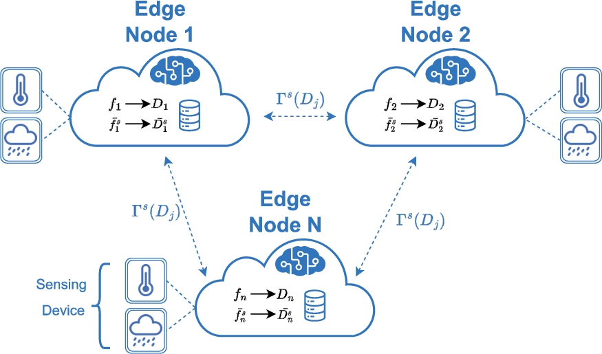
Consider a DML environment depicted in Fig. 1 that comprises n nodes, denoted as N={N1,N2,..,Nn}. While all nodes perform comparable predictive tasks, each node works independently on its unique local dataset defined as Di={(x,y)ℓ}ℓ=1Li, containing Li input-output pairs (x,y)∈X×Y. Notably, the feature vector x=[X1,X2,…,Xd]T∈Rd is d-dimensional and is linked to output y∈Y for regression (e.g. Y⊆R) or classification predictive tasks (e.g. Y⊆{1,2,..,n}). The adjacent ENs of Ni,Nj⊆N∖{Ni}, are a subset of nodes that communicate directly with Ni. In addition, we assume that each node Ni is equipped with two distinct models, a local model fi trained purely on Di and an enhanced model that is built on D˜is data. These enhanced models are built with a varying amount of data from neighboring nodes, which facilitates collaborative learning while preserving data privacy.

Enhanced Models are firstly introduced in [25], that is, for each node Ni and its adjacent nodes Nj, we build enhanced data D˜is={Γs(Di)}∪{Γs(Dj)}, ∀j, j≠i, in which Γs(Dj) represents the information extracted from the original data Dj by using a strategy s. Strategy s controls how our data is extracted from the original distribution Di through statistical learning, dimensionality reduction, compression or DL techniques.

In the context of an enhanced predictive model f˜is, which operates on a set of data Ni and provides predictive services on a data Di, it is important to consider the potential impact of concept drift. Concept drift refers to the possibility that the underlying distribution of data in neighboring nodes, represented by Dj, could change over time. In order to ensure the continued accuracy and reliability of the enhanced model, it is necessary to establish a threshold of error tolerance, denoted as ε. If the difference between the accuracy of the model before and after concept drift, represented by α and α′ respectively, exceeds this threshold (i.e. |α|−|α′|>ε), then the model must be maintained and adapted to the new concept. This consideration is essential for ensuring the continued effectiveness of the enhanced model in practical applications.

Specifically, we aim to assess the effectiveness of enhanced models in handling concept drifts and compare their performances against baseline and local models. Our focus lies on evaluating the impact of introducing a new concept on enhanced model performance, rather than on detecting or understanding concept drifts more generally. To this end, we will simulate abrupt concept drifts, which involve sudden changes in the underlying data distribution, making the effects of concept drift more readily observable. We have identified three distinct types of concept drift simulations, each defined by the relationship between input-output pairs from the original distribution (x and y) and those from the drifted distribution (x′ and y′). In our research, we will be specifically examining the following drift types:

Consider a DML environment with two nodes, denoted as N1 and N2, each of which has its own local model fi and an enhanced model f˜is. Suppose that a concept drift occurs in the data of N2, and the enhanced model f˜1s needs to be maintained as it was built upon the older D2 data. In such a case, the drifted data D2′ must be transmitted through the network to N1 to update the models, resulting in the updated enhanced model f˜1s′. The error L of the updated model is obtained by validating it against the drifted data D2′. Our goal is to minimize the expected error EL(f˜1s′(D2′)) while minimizing inter-node data transmission during maintenance, and ensuring the privacy and security of the user’s data.

4.Maintenance strategies

In this research paper, we present a maintenance approach for our enhanced models, where we leverage the drifted data along a selected strategy to extract information that is used to retrain the enhanced model. We propose different maintenance strategies that can be employed depending on the dataset and predictive tasks performed by the DML system. Our framework comprises strategies that are applicable to regression, multivariate classification, and image classification predictive tasks.

For regression tasks, we adopt on statistical learning approaches, such as clustering, to extract statistics about the underlying data distribution, thereby reducing the number of instances transmitted. For multivariate classification, we primarily rely on dimensionality reduction and compression techniques to transmit the compressed form of the drifted data to the target node, which is then decompressed. Finally, for image classification tasks, we leverage a DL technique to capture the intricate characteristics of computer vision applications.

It is important to note that for all predictive tasks, a baseline (BS) approach exists that involves transmitting raw data over the network. However, this approach violates security constraints and significantly increases the network bandwidth. Our proposed maintenance strategies address these issues and aim to optimize the performance of the DML system while ensuring data security and minimizing network resource utilization. Experimental results demonstrate the effectiveness of our approach in achieving these objectives.

Centroid Guided (CG): The CG approach involves partitioning the input space Dj into K disjoint clusters, where each cluster is represented by its own cluster centroid wjk. In the case of classification data, clustering is performed on the grouped-by-label data, allowing the resulting cluster centroids to be labeled accordingly. The CG strategy involves selecting only the cluster centroids wjk and transmitting them among the ENs:

Enhanced Centroid Guided (ECG): The ECG approach builds upon CG strategy. It starts by partitioning the data space into K clusters and then transfers the resulting cluster centroids wjk to Ni. Next, ECG generates additional samples N(wjk,σj2) around the cluster centroids wjk, where σj2 is the variance of the Gaussian distribution. The resulting set of samples ΓECG(Dj) is then used as the input data of the model when applying the ECG strategy. It is important to note that the value of σj2 must be selected carefully to ensure that the sampled points do not deviate too far from the original distribution of Dj while allowing the model to capture the characteristics of Dj.

Mock Data (MD): The MD approach is a novel strategy that avoids any data transfer to the target node Ni. Instead of sending samples of data, the MD approach substitutes the data with a Linear Regression model fj and additional statistical information such as the mean μj and standard deviation σj of the input space Xj. Training samples Xj¯ are generated on Ni based on the statistics drawn from a Gaussian distribution N(μj,σj2). The Linear Regression model fj is then utilized to obtain the corresponding output pairs as Yj¯=fj(Xj¯)+ϵj, where ϵj is a noise term drawn from a Gaussian distribution that is added to the fj output. Therefore, the MD approach’s sample data (X¯,Y¯) is defined as follows:

Principal Component Analysis (PCA): Our proposed approach employs PCA to reduce the dimensionality of the input space Xj by projecting it onto a low-dimensional space, while still retaining as much information as possible. The first step involves normalizing the input space Xj and computing the eigendecomposition of the covariance matrix Cx=XjXjTn. Subsequently, the eigenvalues are sorted in decreasing order of variance and the data is projected into a lower dimensional space by multiplying the original normalized data by the principal components or the leading eigenvectors. This reduces the amount of information preserved, resulting in greater compression as the number of retained eigenvectors is decreased. The principal components are then transferred to the target node Ni, thereby avoiding the transmission of actual user data and significantly reducing network bandwidth usage. Upon receiving the principal components, the inverse PCA process is initiated to restore the original data format and train the enhanced models. The number of components retained determines how close the decompressed data is to the original Dj. The entire process operates on a group-by-label basis, where the input data Dj is first grouped, and PCA is applied to each distinct labeling group. In this way, we have:

Discrete Cosine Transformation (DCT): Widely used by JPEG as a lossy image compression technique, DCT is utilised as an efficient way of storing our data space Dj upon transmission between the nodes. By applying DCT, the data can be converted into its elementary frequency components. For an input space Dj=f(x,y) with dimensions xL×yL, the 2D-DCT equation can be expressed as:

Our transformation technique does not reduce the number of bits required to represent the data. However, it concentrates the low-frequency coefficients, while setting the other coefficients to zero. When considering an M×N matrix, the most significant coefficients are located at the top-left side of the matrix. By applying this method, a fraction of the most important coefficients is transmitted, while the rest are discarded. As the majority of DCT coefficients have values close to zero, their elimination does not significantly affect the reconstructed nature of the data space Dj′. Following data transfer to Ni, decompression is performed by utilizing inverse DCT to restore the data to its original format, as presented below:

Conditional Variational AutoEncoder (CVAE): It is an enhanced version of the standard Variational AutoEncoder (VAE) that enables the generation of samples conditioned on supplementary input data. The architecture of the CVAE, depicted in Fig. 2, comprises an encoder network, a decoder network, and a latent space.

Fig. 2.

CVAE architecture.

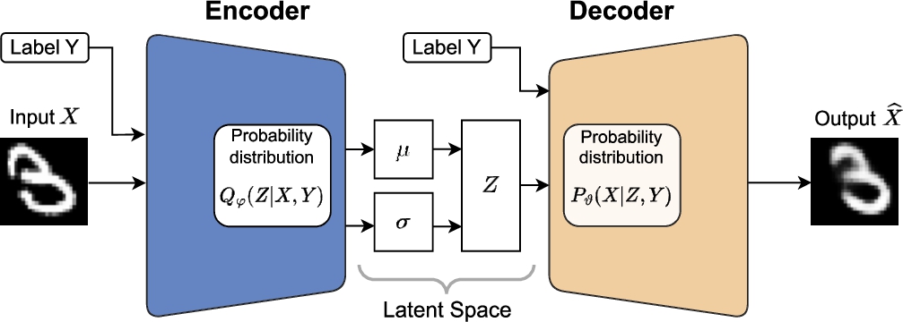
The encoder network takes an input sample X and a conditioning label Y and maps them to the latent vector Z. More specifically, the encoder maps the input data X and the condition label Y to the latent vector Z that follows Gaussian distribution with mean μ and variance σ learned from the input. To achieve this, the encoder output is split into two parts, the mean μ and the variance σ of the Gaussian distribution, which are then used to sample the latent space from the Gaussian distribution. The sampling process introduces stochasticity into the model and helps capture the variations in the data. Formally, let X be the input data and Y be the condition. The encoder maps the input (X,Y) to a distribution over the latent code Z, which follows a Gaussian distribution with mean and variance:

The decoder then maps the latent code Z and the condition Y to a distribution over the data space, which is also modeled as a Gaussian distribution with mean and variance:

During training, the loss function is the negative log-likelihood of the data, which is approximated using the evidence lower bound (ELBO) objective:

5.Experimental evaluation

Our objective is to investigate Problem 1 by examining varying levels of concept drifts and their impact on enhanced models’ performance, and the efficacy of the proposed maintenance strategies in addressing Problem 2. To assess our paradigm, we established three experimental scenarios using real datasets in DML environments.

5.2.Descriptions of the scenarios

We report on the descriptions of the experimentation scenarios, the concept drift simulation and the experimental setup to assess the performance of the proposed framework.

5.2.1.Experimental Scenario I: Regression

Dataset Description: We evaluated our regression scenario upon the real GNFUV multi-node dataset11 adopted by Harth and Anagnostopoulos [11]. The dataset consists of mobile sensors readings over four Unmanned Surface Vehicles (USVs), floating over the sea surface in a testbed in Athens, Greece. Each USV (node) records the measurements such as humidity and temperature of the sea surface, each of which represents an ED within a DML environment. For our experiments, the local data gathered by two of the USVs are employed notated by D1 and D2. Using as input the temperature variable x∈R, we are seeking to predict the humidity which acts as our output variable y∈R.

Simulating Concept Drift: We simulated concept drift in a controlled manner to one of our nodes by employing the three drift types on D2 data. The resulting drifted GNFUV data is illustrated in Fig. 3, where D1 and D2 represent the original data distributions, and D2v′, D2a′, and D2t′ represent the virtual, actual, and total drifted distributions of D2, respectively. This simulation methodology enables us to study the impact of concept drift on ML models and evaluate their robustness in dynamic environments.

Experiment Setup: We conduct experiments by building local fi and enhanced f˜is using the Support Vector Regression (SVR) models and the CG, ECG and MD strategies on the original distributions of the data Di. Subsequently, we examine the impact of each drift type on the enhanced models’ performance and assess the effectiveness of our proposed strategies in mitigating the impact of concept drift. Specifically, we retrain the enhanced model f˜is′ using the drifted data Di′ and re-evaluate its performance against the same drifted data. By analyzing the bandwidth utilization required for maintenance in relation to the performance of the maintained model, we are able to gauge the efficacy of our approach in mitigating the effects of concept drift.

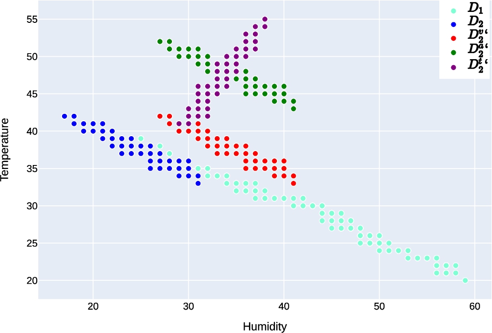
Fig. 3.

Distributions of the GNFUV drifted nodes.

5.2.2.Experimental Scenario II: Multivariate classification

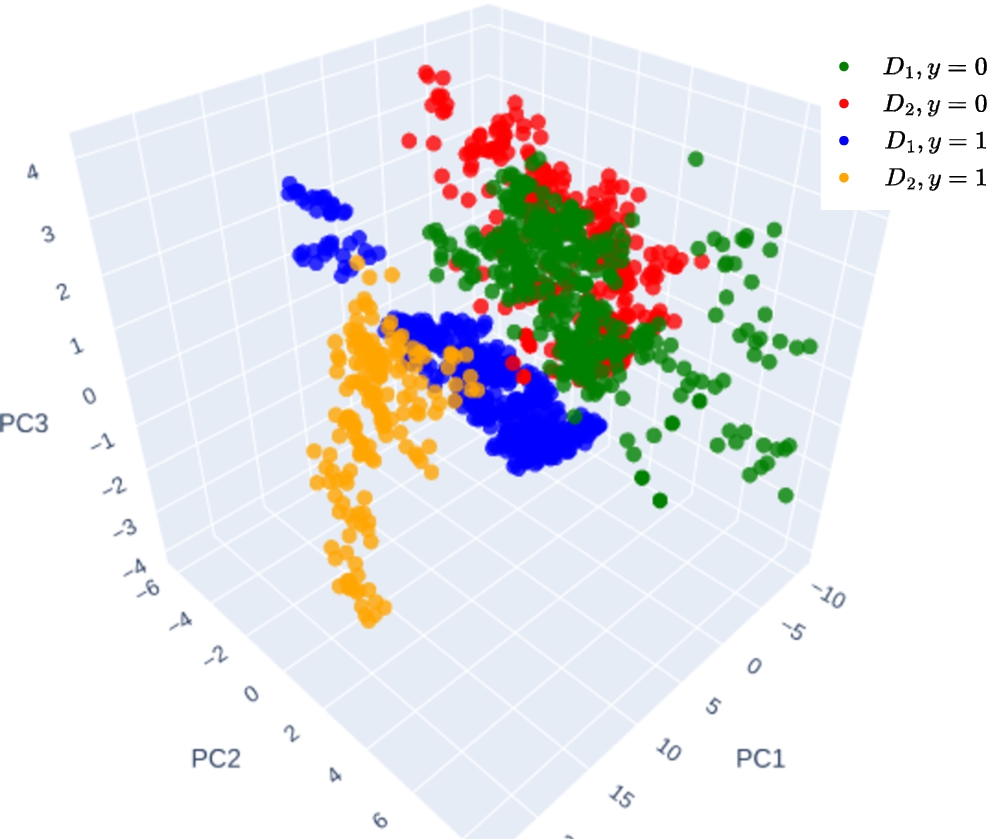
Dataset Description: We also delve into the performance of our resilience framework using the Banknote Authentication (BA) real dataset22 taken from UCI machine learning repository. The present scenario employs a binary classification dataset, consisting of 1372 instances, comprised of image-extracted data from genuine and forged banknote-like specimens. The dataset contains five attributes, with four features and one target attribute and a balanced class distribution ratio of 55:45. In contrast to the GNFUV dataset, the current dataset, lacks an inherent network-node structure. Therefore, the K-means clustering was utilized to construct two nodes. The resulting clusters were designated as D1 and D2, respectively, while preserving the original class distribution of each split data subset. Using as input the 4−dim feature vector x∈R, we are seeking to predict the target attribute which acts as our output variable y⊆{0,1}. Figure 4 depicts the two clustered nodes projected over three Principal Components (PCs).

Simulating Concept Drift: We simulated concept drifts on D2 data using an extension of the actual drift type. We kept P(x) unchanged for all the data, while a certain percentage of P(y) underwent changes in probability. To achieve this, we introduced a parameter α to control the percentage of the data, where its label is swapped. This conversion led to the Actual Drift being converted to P(x)=P(x′)∧α[P(y)≠P(y′)]. To investigate the impact of this parameter on the severity of drift, we conducted experiments using different values of α (0.05, 0.3, and 1), which resulted in the creation of D20.05a′, D20.3a′, and D21a′, respectively. Increasing the value of α led to an increase in the severity of the drift.

Experimental Setup: Our classification models are constructed using the Gaussian Naive Bayes (GaussianNB) algorithm, along with the CG, PCA, and DCT strategies. Upon investigation of the effect of the severity of the concept drift, we update our models to reflect the drifted data D2αa′. We then re-evaluate the performance of our models on the updated data to assess their robustness to concept drift. The results of this experiment provide insights into the effectiveness of the different strategies employed in mitigating the impact of concept drift.

Fig. 4.

Clustered BA dataset projected to 3 PCs.

5.2.3.Experimental Scenario III: Image classification

Dataset Description: In order to investigate the applicability of our framework in more intricate tasks, we conduct an analysis on a Computer Vision classification task using the MNIST dataset33 introduced by LeCun et al. [14]. The dataset contains a set of 70,000 28×28 pixel grayscale images of handwritten digits (0–9), collected by high school students and employees. Similar to the BA dataset, the MNIST dataset lacks an inherent network-node structure, hence we split our dataset into two clusters D1 and D2 comprising of images with labels 0–4 and 5–9, respectively. Using an input image x∈R28×28, we are seeking to predict the handwritten digit y⊆{0,1,2,…,9} of the image.

Simulating Concept Drift: In the current scenario, we simulated concept drift by employing the Virtual drift type to alternate P(x) distribution while keeping P(y) unchanged. Two distinct cases of concept drift are simulated, where the first involves a minor drift by changing the P(x) distribution of the handwritten digit 8 to the P(x′) distribution of the handwritten character B obtained by the EMNIST dataset.44 The second case, which is more severe, involves changing the P(x) distribution of the handwritten digit 9 to the P(x′) distribution of the handwritten character K. In both cases, the labels are unchanged and the simulated concept drifts are identified as D2v′8→B and D2v′9→K, respectively.

Experimental Setup: We used a Multi-Layer Perception (MLP) classifier consisting of three linear layers and ReLU activations functions. This allowed us to learn complex non-linear relationships between the input features x∈R28×28 and the output classes y⊆{0,1,2,…,9} of the images. The CVAE strategy is employed for the training of the enhanced models f˜iCVAE, where the two concept drift scenarios are evaluated. The CVAE model fθ(Zi) is trained on each node’s local data Di, capturing the characteristics of the data and modeling the latent space Zi. The CVAE network architecture consisted of three linear layers for the encoding part and 2 linear layers for the decoding part, utilizing the Exponential Linear Unit (ELU) function and sigmoid activation functions between the layers.

The experimental procedure for the training of the enhanced models consisted of four steps: (i) training a CVAE model fθ(Zi) on each node’s local data Di, (ii) transferring the latent space Zi to the target node Nj, (iii) generating new sample images based on the Zi latent space using the labels of the Di data on Nj node, and (iv) using the newly generated images along with the decoded images of the Nj node, train the f˜jCVAE enhanced model. The visual comparison presented in Fig. 5 pertains to images possessing a label value of 5. Specifically, the figure displays three images: an original MNIST image (5a), the corresponding decoded image generated by the CVAE (5b), and a novel generated image sample produced by the CVAE (5c).

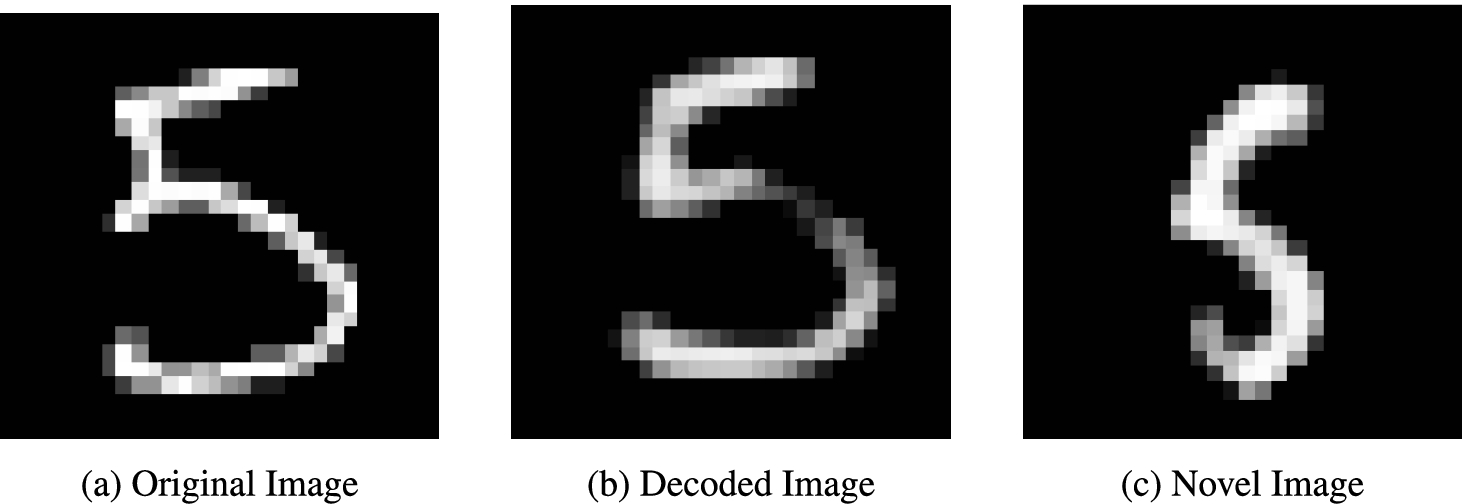
Fig. 5.

MNIST images with a label value of 5.

In cases where concept drift is detected, a new CVAE model fθ′(Zi) is trained, forming a new latent space Zi′. The procedure then resumed from point (ii) to ensure that the enhanced model f˜jCVAE′ can accurately perform on the drifted data Di′. The present methodology offers a practical approach for the training and maintenance of enhanced models that can proficiently handle concept drifts. By implementing the CVAE strategy, the transmission of data across the network is minimized as solely the latent space is transferred instead of a voluminous amount of raw images, which holds significant promise for reducing computational requirements in EC.

5.3.Comparative assessment

5.3.1.Concept drift effects on enhanced models

We first analyze the effect of concept drift on the efficacy of enhanced models, as well as its correlation with local models. Furthermore, we seek to delve deeper into this impact and its relationship with the strategies employed in constructing the enhanced models. Through this analysis, we aim to provide valuable insights into the nuances of concept drift and its implications for model performance.

Scenario I: To examine the impact of concept drifts on the performance of the enhanced model, we conducted experiments by combining the original D2 data with the drifted D2′ data, followed by applying our enhanced models trained on the original D2 data. It is important to note that our incoming data are delivered in batches of 100 data points, with a sliding window of 10 data points.

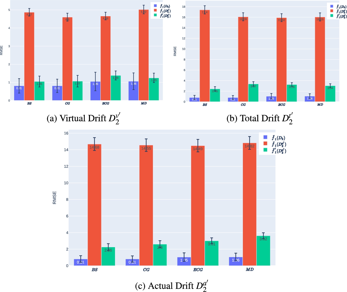
The outcomes of the study in Scenario I reveal the mean RMSE performance of the local and enhanced models for each concept drift type, as indicated in Table 1. Additionally, Fig. 6 showcases the performances of f˜1, constructed by each strategy per batch of the three drift types.

Table 1

Scenario I mean models’ performance by drift

	RMSE
Model	D2	D2v′	D2a′	D2t′
f2	0.42±0.04	5.31±0.26	14.80±0.77	17.53±0.76
f˜1BS	0.81±0.40	4.87±0.21	14.86±0.78	16.40±0.80
f˜1CG	0.81±0.37	4.60±0.22	14.55±0.76	16.09±0.78
f˜1ECG	1.05±0.51	4.66±0.21	14.49±0.75	15.92±0.78
f˜1MD	1.06±0.46	5.02±0.24	14.82±0.77	16.05±0.78

Fig. 6.

Performance of f˜1 against D2, D2v′, D2a′ and D2t′ batches of data.

The analysis of the results presented in Table 1 reveals that the local model f2 performs better on the original distribution; however, it is less generalizable and hence more susceptible to the negative effects of concept drift. In contrast, the enhanced models exhibit lower quality of service on the original distribution, with a less severe performance drop when confronted with concept drift as compared to f2.

Furthermore, it is worth noting that the strategies employed to construct the enhanced models do not appear to have a significant impact on the effect of concept drift, as evidenced in Fig. 6, where all the enhanced models exhibit similar trends and patterns. Moreover, the experimental findings indicate that D2v′ has the least detrimental effect on model performance, while D2t′ has the most severe effect, thereby corroborating the order of severity of the drift types being D2v′, D2a′ and D2t′ in ascending order.

Scenario II: In this study, we conducted multivariate classification using the distribution D2 and its drifted counterpart D2′. Specifically, we concatenated these two datasets to evaluate the performance of our enhanced models before and after concept drift, following a similar approach to Scenario I. We used a batch size of 100 and a sliding window size of 10 throughout the experiment. Table 2 presents the average performance of the local and enhanced models before and after the occurrence of concept drift for each drift type. In addition, we visualize the accuracy per batch and the performance drop of the enhanced models f˜1 upon the emergence of novel concepts in Fig. 7.

Table 2

Scenario II mean models’ performance by drift

	Accuracy (%)
Model	D2	D20.05a′	D20.3a′	D21a′
f2	98.05±1.68	93.68±1.57	68.82±6.84	1.59±0.74
f˜1BS	95.77±1.73	92.44±1.69	68.86±9.21	3.30±2.05
f˜1CG	93.75±2.36	90.31±2.70	69.37±7.85	1.38±1.07
f˜1PCA	95.52±1.55	92.36±1.62	68.43±8.15	4.14±2.17
f˜1DCT	96.60±1.78	93.47±1.25	69.31±8.30	3.00±1.92

Fig. 7.

Performance of f˜1 against D2, D20.05a′, D20.3a′ and D21a′ batches of data.

Our results indicate that similar to Scenario I, the local model outperforms the enhanced models by a small margin of approximately 3%. On the other hand, and in contrast to Scenario I, the enhanced models provide the same level of generalizability as the local model. That is, both the local and enhanced models exhibit comparable predictive service quality in the presence of concept drift. Interestingly, we did not observe any improvement in the performance of the enhanced models as compared to the local model after the occurrence of concept drifts, which was consistent with our expectations. This observation may be attributed to the characteristics of the BA dataset or the lack of an inferent network-node structure in the dataset, as opposed to the GNFUV dataset used in Scenario I.

We also found that the parameter α, which was introduced to the formula of the Actual Drift, is correlated with the performance drop of the model. When α was set to 5%, we observed a corresponding drop in accuracy of approximately 5%, which was consistent across all drift cases. Finally, by analyzing the accuracy of the enhanced models over batches of incoming data in Fig. 7, we reveal a consistent trend, indicating that the strategies employed to construct the enhanced models are independent of the performance drop.

Scenario III: In this scenario, we conducted an evaluation of the image classification predictive task. To ensure consistency with our previous evaluation procedures, we followed the same methodology for this scenario. Specifically, we concatenated the original dataset D2 with the drifted datasets D2′ and evaluated and tested our models on the incoming data in batches of 64 images. The experimental results are presented in Table 3, while Fig. 8a illustrates the accuracy per batch plot of the baseline enhanced model f˜1BS. Furthermore, the accuracy per batch of the local f2 and enhanced f˜1CVAE models are presented in Fig. 8b.

Table 3

Scenario III mean model’s performance by drift

	Accuracy (%)
Model	D2	D2v′8→B	D2v′9→K
f2	98.57±1.45	88.83±4.05	78.17±5.38
f˜1BS	97.51±2.03	91.11±3.81	87.76±4.01
f˜1CVAE	90.65±3.57	83.00±4.42	82.37±4.73

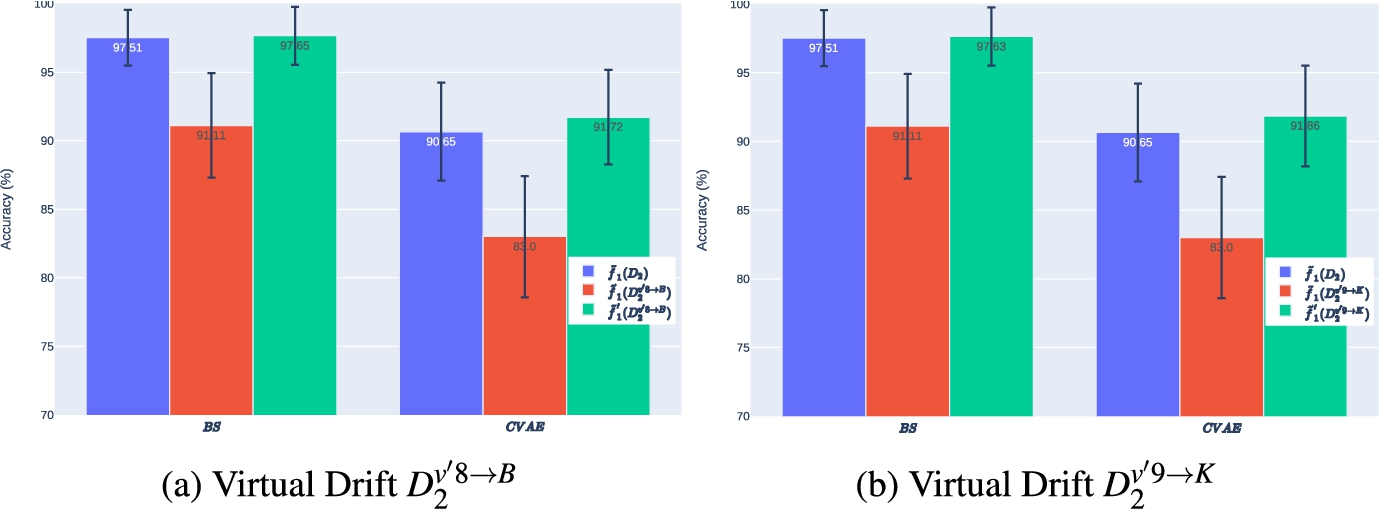
Fig. 8.

Models performances against D2, D2v′8→B and D2v′9→K batches of data.

Upon observing f2 in both Table 3 and Fig. 8b, it is apparent that the model experiences a drop in accuracy of 10% and 20% on drifts D2v′8→B and D2v′9→K, respectively. Notably, the more severe drift, D2v′9→K, resulted in a twice larger decrease in model performance compared to the less severe drift, D2v′8→B. Similarly, f˜1BS exhibits a reduction in accuracy of approximately 5% and 10% on D2v′8→B and D2v′9→K, respectively. These findings suggest that f˜1BS is less vulnerable to the effects of concept drifts compared to f2.

On the other hand, the experimental results reveal that the performance of f˜1CVAE is not as high as f2 and f˜1BS. However, an interesting finding is that the severity of the drift does not correlate with the performance drop of the model, indicating that f˜1CVAE is less vulnerable to the effects of concept drifts. Specifically, the performance of f˜1CVAE remains relatively consistent across both less severe (D2v′8→B) and more severe (D2v′9→K) drifts, which is better than the performance of the local model f2 in some cases. This can be explained by the fact that during the training of the CVAE and generation of novel images, certain characteristics of the drifted dataset deteriorate in scale, making f˜1CVAE more generalizable and less susceptible to the effects of concept drifts. In other words, the CVAE’s ability to learn and generate novel images that capture the underlying characteristics of the drifted dataset allows it to maintain its performance across different drift types, making it a promising approach for dealing with concept drifts in image classification scenarios.

5.3.2.Enhanced models maintenance

In this phase of our evaluation, we employ all types of drifted data D2′ to preserve our enhanced models and examined the impact of our proposed maintenance strategies on the performance of the enhanced models over the drifted data. Furthermore, we analyze how these strategies mitigate inter-node data transmission during the maintenance of an enhanced model. Consequently, we assess the trade-off between the performance of the maintained enhanced models and the volume of data transmitted over the DML network required to sustain our models.

Fig. 9.

Average performance of f˜1 and maintained f˜1′ against D2 and D2′.

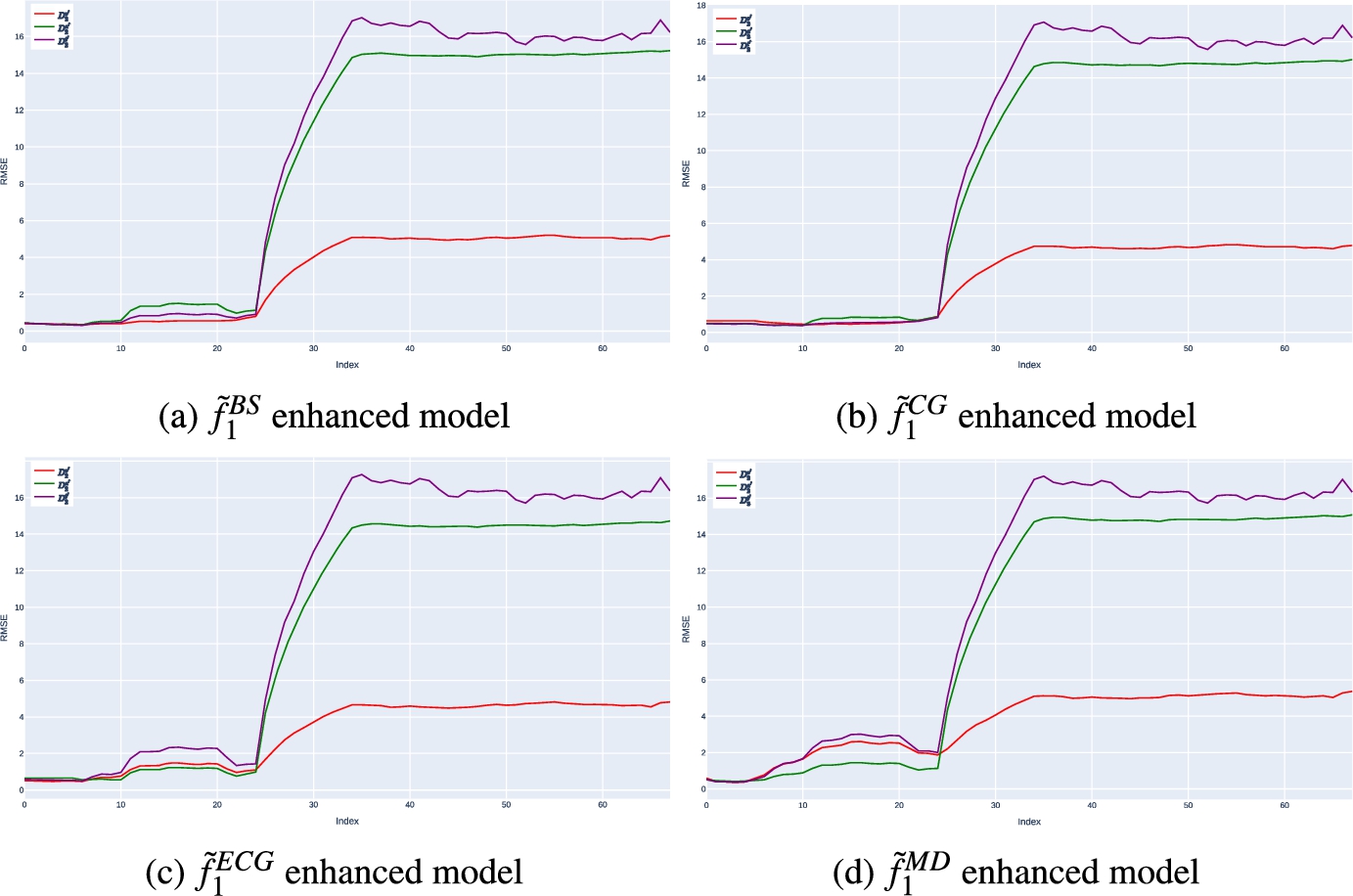
Scenario I: Fig. 9 showcases the outcomes of our analysis. The plot displays the performance of the initial enhanced model over the original D2 data, the performance of the same model on the drifted D2′ data, and the performance of the maintained enhanced model against the drifted D2′ data where the virtual, total and actual drift types are employed. Additionally, we demonstrated the trade-off between the performance and network throughput ratio in Fig. 10. The performance denotes the mean RMSE score of the maintained enhanced models over the drifted data, while the network throughput ratio represents the ratio of the bit-wise data requirements for the maintenance of the baseline enhanced model in comparison to the maintenance of the enhanced models generated by the other strategies.

Upon examining the performances of the enhanced models before and after the occurrence of concept drift, it is apparent that superior performance of f˜1(D2) corresponds to better performance of f˜1′(D2′). However, there exists a marginal increase in the mean RMSE value of the f˜1′(D2′) as compared to f˜1(D2), across all the different drift types. Furthermore, it is noteworthy that the magnitude of the RMSE increase can be related to a proportional manner to the severity of the drift, as this marginal increase is more for the actual and total drifts. Among the three employed strategies, f˜1CG emerged as the best-performing approach, disregarding the inter-node data requirements essential for enhanced model maintenance. It outperformed the other strategies and achieved performance similar to that of the baseline.

Fig. 10.

Performance of f˜1′ against D2v′, D2a′ and D2t′ given different ratio of the inter-node data transmission.

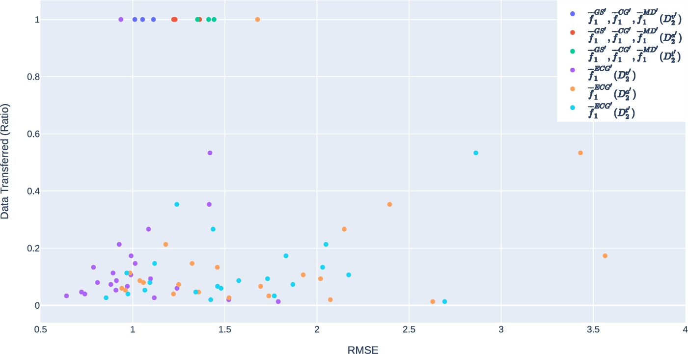
Figure 10 illustrates the RMSE performance of the f˜1S′ enhanced model after maintenance over drifted D2′ data types using the different maintenance strategies. One could observe that the severity of the drift types correlates with the increase of the RMSE value, regardless of the value of the data transferred ratio. However, as evidenced, the data compression ratio over the ECG strategy is not associated in a proportional manner with the overall performance of the enhanced model. The results demonstrate that the enhanced model’s performance is adversely affected by either a very small or a very large number of cluster centroids used. In the latter, the high number of cluster centroids and hence the small number around them, overfit the enhanced models. While, in the former case, there are too few cluster centroids to adequately capture the characteristics of the dataset, leading to under-fitting. Accordingly, the best trade-off lies within the 0.1 data transmission ratio, which scores a lower RMSE for each type of drift. In this way, our framework achieves similar performance with GS, CG, and MD strategies while transferring 10 times fewer data in the network.

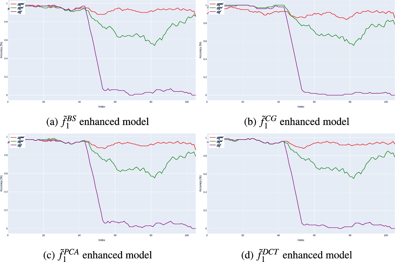
Scenario II: This section presents the experimental results of our analysis on a multivariate classification scenario over the BA dataset, obtained after the maintenance of the enhanced models. Figure 11 presents the maintained performance of the models for D20.05a′, D20.3a′ and D21a′. As in Scenario I, a trade-off plot is depicted in Fig. 14.

Fig. 11.

Average performance of f˜1 and maintained f˜1′ against D2 and D20.05a′, D20.3a′ and D21a′.

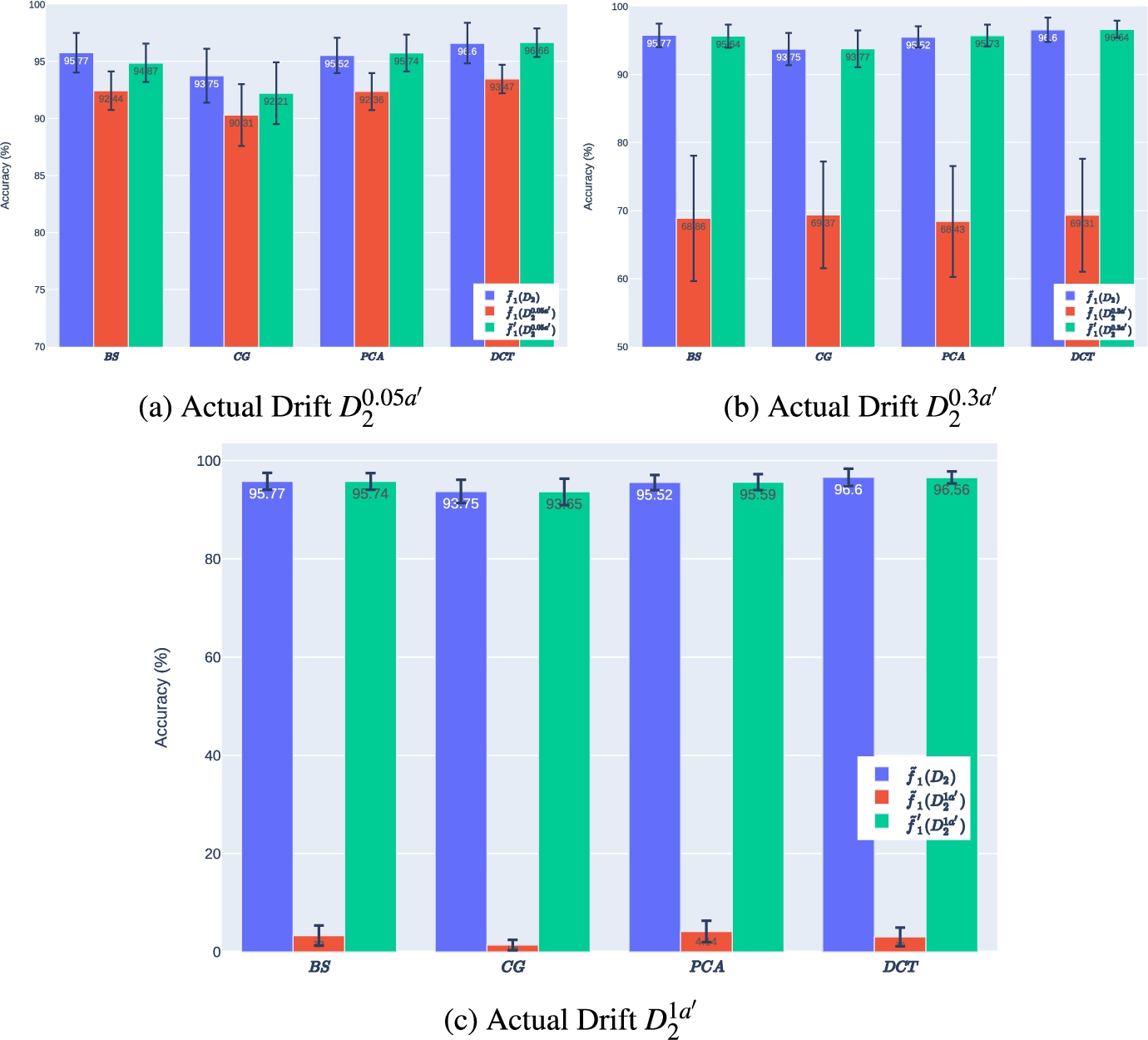
It can be observed that the slight deterioration in the performance of the maintained enhanced models, as witnessed in Scenario I, is no longer evident. This is due to the fact that certain enhanced models after maintenance f˜1′(D20.3α′), exhibit better performance than f˜1(D2). Furthermore, in contrast to Scenario I, it is noteworthy that the CG strategy performed the worst out of the three maintenance strategies employed in this scenario. On the other hand, the enhanced models built using compression and dimensionality reduction techniques displayed better performances. Among the three strategies employed in this phase, the enhanced model built using the DCT strategy emerged as the best, while the PCA strategy came second, with its performance being comparable to the baseline. Our findings demonstrate that the maintenance strategies employed in our analysis have a significant impact on the performance of the enhanced models. The enhanced models built upon compression techniques were able to overcome the performance deterioration observed in Scenario I, and in some cases, outperformed the baseline model.

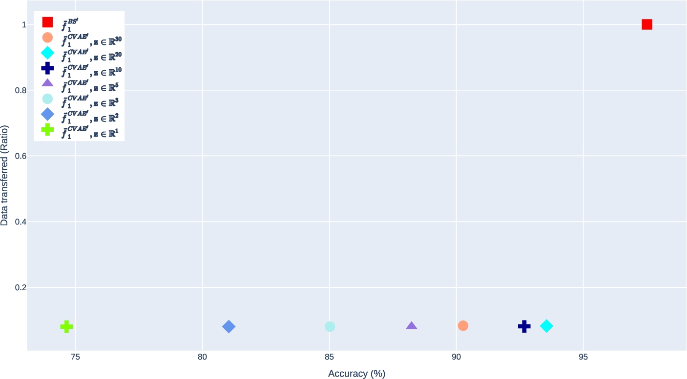
In this section, we focus on the trade-off plot presented in Fig. 12, which provides insights into the relationship between model performance and inter-node data transmission. Specifically, we examine the right-bottom corner of the plot where models achieve superior performance with less inter-node data transmission. To identify the optimal parameters for each maintenance strategy, we explore several parameters that push the boundaries of the models while avoiding those with poor performance. Our experimentation begins with f˜1PCA′, where we gradually remove one dimension at a time. Our findings demonstrate that even by projecting the dataset into lower dimensions, there is a significant reduction in inter-node data transmission without compromising the performance of the model. However, while projecting the data onto a single dimension achieved superior performance, there exist other strategies that can achieve the same or even better performance while transferring fewer data. Therefore, enhanced models constructed using the PCA strategy can help reduce the inter-node data requirements for sustainable models while simultaneously achieving high-quality service. Nevertheless, in this scenario, it is not the optimal strategy.

Fig. 12.

Performance of f˜1′ against D20.3a′ given different ratio of the inter-node data transmission.

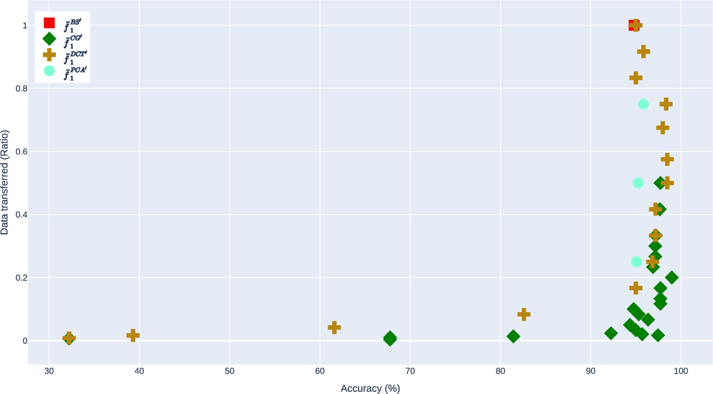
Upon careful examination of the performance of the f˜1DCT′, we observed a correlation between the amount of data transmitted and the model’s performance. We found that when the dataset remains almost untouched upon transmission, the model’s performance is comparable to the baseline. However, when fewer frequency coefficients are transmitted over the network, the generalizability of f˜1DCT′ improves, resulting in more accurate results. The optimal performance of the model is achieved when the ratio of transmitted data is between 0.2–0.7. When the ratio is less than 0.2, the model’s performance starts to deteriorate, as not enough coefficients are transmitted to capture the characteristics of the BA dataset. A similar observation was made regarding the performance of f˜1CG′. The CG strategy achieved the least amount of data transmission among all the strategies, while performing the best out of all the enhanced models. We found that the optimal data transfer ratio for this model was around 0.02–0.2, resulting in accuracies above 95%, with some cases close to 100%.

Our analysis revealed that all the strategies we tested achieved a substantial reduction in the amount of data required to be transmitted over the network during the maintenance of our enhanced models. We observed instances where our strategies transferred significantly less data compared to the baseline. Notably, the CG strategy stood out as the most effective strategy in terms of data transfer ratio and accuracy performance of the enhanced model. This strategy reduced data transmission by up to 50 times while achieving better accuracy than the baseline.

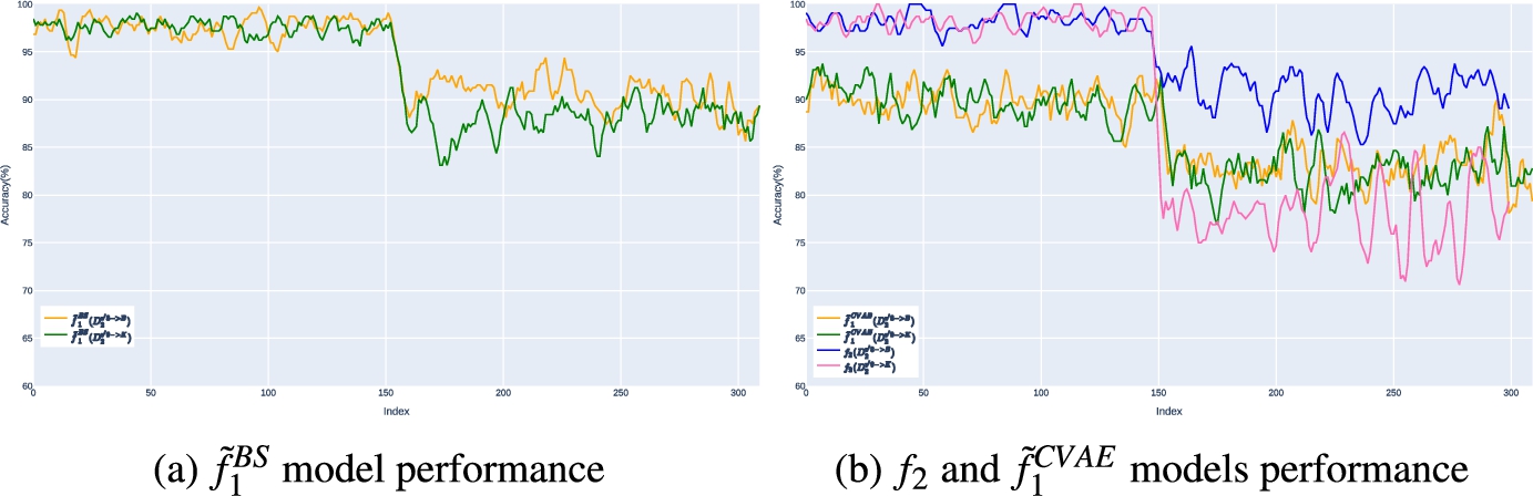
Scenario III: This study presents an experimental analysis of the performance of enhanced models before and after maintenance in the image classification scenario. The performance of the enhanced models over D2v′8→B is plotted in Fig. 13a, while the same analysis is presented over D2v′9→K in Fig. 13b. Additionally, to evaluate the trade-off between the models’ performance and inter-node data transmission, we exploited different latent space Z dimensions as illustrated in Fig. 14.

Through a comparative analysis of the performance of f˜1(D2) and f˜1′(D2v′8→B) using both baseline and CVAE strategies, we can observe that the enhanced models’ performance is improved by a slight margin. These improvements are significant as they enable the models to maintain and enhance the quality of service even after encountering drift. While it is true that f˜1BS provides higher accuracy levels for both pre and post-maintenance scenarios, it is important to note that the performance of f˜1CVAE can still be deemed acceptable, especially considering the benefits of reduced inter-node data requirements, as analyzed in the subsequent sections.

Fig. 13.

Average performance of f˜1 and maintained f˜1′ against D2 and D2v′.

The construction and maintenance of f˜1BS involved using approximately 5000 labeled images from D1 with labels 0–4 and another 5000 labeled images from D2 with labels 5–9. These images were transferred over the DML network to train the model, which corresponds to an average of 1000 images per label, considering that the MNIST dataset has ten labels.

However, for the construction and maintenance of f˜1CVAE, we did not transfer the raw images. Instead, we transferred the latent space Z, which is required to generate new images from the trained CVAE model. The generation of new images requires knowledge of the decoder network’s parameters θ and the prior distribution P(Z) over the latent space. The number of parameters θ depends on the number of layers, their corresponding input and output dimensions, and the number of bias parameters, which is the same as the number of outputs for each linear layer. The byte-wise data requirements upon a concept drift maintenance scenario for f˜1CVAE, are presented in Table 4. The table also displays the byte-wise data requirements for transferring 5000 MNIST images over the network, used for the baseline solution. To calculate the number of parameters θ for each decoder network, we multiplied the input and output features of each linear layer. We assume that the commonly used 32-bit floating-point precision (float32) is used to represent the parameters θ, which means that each parameter requires 4 bytes of storage.

Table 4

Byte-wise data requirements for the construction and maintenance of f˜1′ per strategy

Strategy	Z dimensions	Parameters θ	Bytes
BS	–	–	15,860,000
CVAE	30	326,784	1,307,136
CVAE	20	322,784	1,291,136
CVAE	10	318,784	1,275,136
CVAE	5	316,784	1,267,136
CVAE	3	315,984	1,263,936
CVAE	2	315,584	1,262,336
CVAE	1	315,184	1,260,736

Fig. 14.

Performance of f˜1′ against D2v′8→B given different ratio of the inter-node data transmission.

Based on the results presented in Table 4 and Fig. 14, it can be concluded that the dimensionality of the latent space Z does not have a significant impact on the inter-node data transmission. However, it does play a critical role in the performance of the enhanced models. Among the enhanced models constructed using the CVAE strategy, it was observed that f˜1CVAE′, z∈R20 achieved the best performance, with f˜1CVAE′, z∈R10 and f˜1CVAE′, z∈R30 following closely in second and third place, respectively. Models with a latent space dimensionality of less than 5 could not adequately provide quality predictive services. Hence, our optimal number of latent space dimensions is 20, as demonstrated by the f˜1CVAE′ model, which achieved a mean accuracy of approximately 94%, 3% less than the baseline, while transferring roughly 12 times fewer data. It is worth noting that these calculations are based on the transfer of 5000 images between the nodes, and the benefits of the CVAE strategy can be further amplified when constructing enhanced models using more images.

These findings demonstrate the practical implications of using CVAE over the traditional baseline approach, as the byte-wise data requirements for transferring latent space Z are substantially lower than those for transferring raw images. This is an important consideration when designing systems that must operate efficiently and with minimal network utilization.

6.Conclusion

In this research, we addressed the problem of model maintenance in a DML environment, where models must adapt to changes in the data distribution over time. Specifically, we proposed a framework that constructs enhanced models to aid failed nodes in their predictive analytics services and introduced maintenance strategies to sustain the quality of service of the enhanced models in the presence of concept drifts, in a lightweight yet effective manner. Our method can work together with federated learning, especially for making federated learning resilient and robust when it comes to node failures and concept drifts.

To evaluate the effectiveness of our proposed framework and maintenance strategies, we conducted three experimental scenarios over three real datasets with different predictive analytics tasks, including regression, multivariate classification, and image classification. For each scenario, we proposed maintenance strategies that are applicable to each task and simulated different types of concept drifts in a controlled manner.

We divided our experimental evaluation into two phases. In the first phase, we investigated how the performance of the enhanced model is affected under different severities of concept drift and how this correlates with the performance effects of local models. We found that the enhanced model exhibited increased generalizability, resulting in less impact on predictability performance when facing a concept drift as compared to local models. Moreover, the severity of concept drift correlated with the performance drop of the enhanced models. Importantly, we also found that the strategies adopted to construct the enhanced model did not significantly impact its performance, as all of them exhibit similar trends and patterns.

In the second phase of our experimental evaluation, we validated the applicability of our proposed maintenance strategies by retraining the models with the novel trends encountered after a concept drift. Our findings suggest that the trade-off between the inter-node data transmission volume and performance loss can be effectively managed by selecting a suitable maintenance strategy that balances the need for data reduction with the preservation of model performance. Different scenarios yielded different optimal strategies, but all performed similarly or even better than the baseline, achieving a substantial reduction in the amount of data required to be transmitted over the network during the maintenance of the enhanced models.

Our future agenda includes exploring several areas to improve upon our framework and extend its applicability to a wider range of DML scenarios. One important direction is to expand the scope of our experimental evaluation beyond the limited two-EN setting, and explore the applicability of the enhanced model to aid multiple failed nodes in more complex DML environments. This would provide a more comprehensive understanding of the framework’s effectiveness and limitations, and enable us to further optimize the maintenance strategies for the enhanced models in such scenarios. Another promising direction is to investigate the applicability of other conditional generative models, such as Conditional Generative Adversarial Network (cGAN) and Conditional PixelCNN, which could help improve the framework’s capabilities in generating high-quality images, and thereby improve the predictability performance of the enhanced models. While our study has focused on VAE-based conditional generative models, cGANs and Conditional PixelCNN have been shown to have high-quality image generation capabilities, and could be explored for image-based predictive analytics tasks.

Conflict of interest

None to report.

References

[1] | A.A. Abdellatif, A. Mohamed, C.F. Chiasserini, M. Tlili and A. Erbad, Edge computing for smart health: Context-aware approaches, opportunities, and challenges, IEEE Network 33: (3) ((2019) ), 196–203. doi:10.1109/MNET.2019.1800083. |
[2] | S.H. Bach and M.A. Maloof, Paired learners for concept drift, in: 2008 Eighth IEEE International Conference on Data Mining, IEEE, (2008) , pp. 23–32. doi:10.1109/ICDM.2008.119. |
[3] | M. Baena-Garcıa, J. del Campo-Ávila, R. Fidalgo, A. Bifet, R. Gavalda and R. Morales-Bueno, Early drift detection method, in: Fourth International Workshop on Knowledge Discovery from Data Streams, Vol. 6: , (2006) , pp. 77–86. |
[4] | S. Bouarourou, A. Zannou, A. Boulaalam and E.H. Nfaoui, Iot based smart agriculture monitoring system with predictive analysis, in: 2022 2nd International Conference on Innovative Research in Applied Science, Engineering and Technology (IRASET), (2022) , pp. 1–5. |
[5] | J. Deogirikar and A. Vidhate, Security attacks in iot: A survey, in: 2017 International Conference on I-SMAC (IoT in Social, Mobile, Analytics and Cloud) (I-SMAC), IEEE, (2017) , pp. 32–37. doi:10.1109/I-SMAC.2017.8058363. |
[6] | P. Domingos and G. Hulten, Mining high-speed data streams, in: Proceedings of the Sixth ACM SIGKDD International Conference on Knowledge Discovery and Data Mining, (2000) , pp. 71–80. doi:10.1145/347090.347107. |
[7] | R. Elwell and R. Polikar, Incremental learning of concept drift in nonstationary environments, IEEE Transactions on Neural Networks 22: (10) ((2011) ), 1517–1531. doi:10.1109/TNN.2011.2160459. |
[8] | I. Frías-Blanco, J.d. Campo-Ávila, G. Ramos-Jiménez, R. Morales-Bueno, A. Ortiz-Díaz and Y. Caballero-Mota, Online and non-parametric drift detection methods based on Hoeffding’s bounds, IEEE Transactions on Knowledge and Data Engineering 27: (3) ((2015) ), 810–823. doi:10.1109/TKDE.2014.2345382. |
[9] | J. Gama and G. Castillo, Learning with local drift detection, in: Advanced Data Mining and Applications, X. Li, O.R. Zaïane and Z. Li, eds, Springer, Berlin Heidelberg, (2006) , pp. 42–55. |
[10] | J. Gama, P. Medas, G. Castillo and P. Rodrigues, Learning with drift detection, in: Lecture Notes in Computer Science (Including Subseries Lecture Notes in Artificial Intelligence and Lecture Notes in Bioinformatics), vol. 3171: , (2004) , pp. 286–295. |
[11] | N. Harth and C. Anagnostopoulos, Edge-centric efficient regression analytics, in: 2018 IEEE International Conference on Edge Computing (EDGE), (2018) , pp. 93–100. |
[12] | G. Hulten, L. Spencer and P. Domingos, Mining time-changing data streams lau ries @ innovation-next.corn, 2001. |
[13] | S. Krishnan, S. Venkatasubramanian, T. Dasu and K. Yi, An information-theoretic approach to detecting changes in multidimensional data streams an information-theoretic approach to detecting changes in multi-dimensional data streams, 2014. |
[14] | Y. Lecun, L. Bottou, Y. Bengio and P. Haffner, Gradient-based learning applied to document recognition, Proceedings of the IEEE 86: (11) ((1998) ), 2278–2324. doi:10.1109/5.726791. |
[15] | A. Liu, Y. Song, G. Zhang and J. Lu, Regional concept drift detection and density synchronized drift adaptation, in: IJCAI International Joint Conference on Artificial Intelligence, (2017) . |
[16] | J. Lu, A. Liu, F. Dong, F. Gu, J. Gama and G. Zhang, Learning under concept drift: A review, IEEE Transactions on Knowledge and Data Engineering 31: ((2019) ), 2346–2363. |
[17] | N. Lu, G. Zhang and J. Lu, Concept drift detection via competence models, Artificial Intelligence 209: ((2014) ), 11–28. doi:10.1016/j.artint.2014.01.001. |
[18] | H. Luo, H. Cai, H. Yu, Y. Sun, Z. Bi and L. Jiang, A short-term energy prediction system based on edge computing for smart city, Future Generation Computer Systems 101: ((2019) ), 444–457. doi:10.1016/j.future.2019.06.030. |
[19] | K. Nishida and K. Yamauchi, Detecting concept drift using statistical testing, in: International Conference on Discovery Science, Springer, (2007) , pp. 264–269. |
[20] | A. Qahtan, B. Alharbi, S. Wang and X. Zhang, A pca-based change detection framework for multidimensional data streams, in: Proceedings of the ACM SIGKDD International Conference on Knowledge Discovery and Data Mining 2015-August, Vol. 8: , (2015) , pp. 935–944. |
[21] | N.P. Rana, S. Luthra, S.K. Mangla, R. Islam, S. Roderick and Y.K. Dwivedi, Barriers to the development of smart cities in Indian context, Information Systems Frontiers 21: ((2019) ), 503–525. doi:10.1007/s10796-018-9873-4. |
[22] | J.C. Schlimmer and R.H. Granger, Incremental learning from noisy data, Machine Learning 1: (3) ((1986) ), 317–354. |
[23] | A. Tsymbal, M. Pechenizkiy, P. Cunningham and S. Puuronen, Dynamic integration of classifiers for handling concept drift, Information fusion 9: (1) ((2008) ), 56–68. doi:10.1016/j.inffus.2006.11.002. |
[24] | M.Q. Wang, D.C. Anagnostopoulos, J. Fornes, D.K. Kolomvatsos and M.A. Vrachimis, Maintenance of model resilience in distributed edge learning environments, in: 19th IEEE International Conference on Intelligent Environments (IE’23), (2023) . |
[25] | Q. Wang, J.M. Fornes, C. Anagnostopoulos and K. Kolomvatsos, Predictive model resilience in edge computing, 2022. |
[26] | G.I. Webb, R. Hyde, H. Cao, H.L. Nguyen and F. Petitjean, Characterizing concept drift, Data Mining and Knowledge Discovery 30: ((2016) ), 964–994. doi:10.1007/s10618-015-0448-4. |
[27] | E. Welbourne, L. Battle, G. Cole, K. Gould, K. Rector, S. Raymer, M. Balazinska and G. Borriello, Building the internet of things using rfid: The rfid ecosystem experience, IEEE Internet computing 13: (3) ((2009) ), 48–55. doi:10.1109/MIC.2009.52. |
[28] | S. Xu and J. Wang, Dynamic extreme learning machine for data stream classification, Neurocomputing 238: ((2017) ), 433–449. doi:10.1016/j.neucom.2016.12.078. |
[29] | T. Xu, G. Han, X. Qi, J. Du, C. Lin and L. Shu, A hybrid machine learning model for demand prediction of edge-computing-based bike-sharing system using internet of things, IEEE Internet of Things Journal 7: (8) ((2020) ), 7345–7356. doi:10.1109/JIOT.2020.2983089. |
[30] | E.P. Yadav, E.A. Mittal and H. Yadav, Iot: Challenges and issues in indian perspective, in: 2018 3rd International Conference on Internet of Things: Smart Innovation and Usages (IoT-SIU), IEEE, (2018) , pp. 1–5. |
[31] | S. Yu, X. Wang and J.C. Principe, Request-and-reverify: Hierarchical hypothesis testing for concept drift detection with expensive labels, in: IJCAI International Joint Conference on Artificial Intelligence 2018-July, Vol. 6: , (2018) , pp. 3033–3039. |