
HighNESS conceptual design report: Volume II. The NNBAR experiment.
Abstract
A key aim of the HighNESS project for the European Spallation Source is to enable cutting-edge particle physics experiments. This volume presents a conceptual design report for the NNBAR experiment. NNBAR would exploit a new cold lower moderator to make the first search in over thirty years for free neutrons converting to anti-neutrons. The observation of such a baryon-number-violating signature would be of fundamental significance and tackle open questions in modern physics, including the origin of the matter-antimatter asymmetry. This report shows the design of the beamline, supermirror focusing system, magnetic and radiation shielding, and anti-neutron detector necessary for the experiment. A range of simulation programs are employed to quantify the performance of the experiment and show how background can be suppressed. For a search with full background suppression, a sensitivity improvement of three orders of magnitude is expected, as compared with the previous search. Civil engineering studies for the NNBAR beamline are also shown, as is a costing model for the experiment.
1.List of acronyms
See Table 1.
Table 1
List of acronyms
| Acronym/term | Meaning |
| BNV | Baryon number violation |
| CAD | Computer Aided Design |
| COMSOL | A finite element analysis and simulation software package |
| CDR | Conceptual design report |
| DAQ | Data aquisition system |
| ESS | European Spallation Source |
| FOM | Figure of merit |
| GEANT4 | A Monte Carlo simulation program for GEometry ANd Tracking |
| HighNESS | High intensity Neutron Source at the European Spallation Source |
| HRD | Hadronic range detector |
| ILL | Institut Laue Langevin |
| LDA | Linear Discriminant Analysis |
| LEC | Lead-glass electromagnetic calorimeter |
| LBP | Large beamport |
| Liquid deuterium | |
| MCNP | Monte Carlo N Particle |
| MCPL | Monte Carlo Particle Lists |
| MCStas | Monte Carlo simulation of neutron instruments |
| ML | Machine Learning |
| MP | Monoplanar reflector |
| NNBAR | An experiment to search for neutrons converting to antineutrons at the ESS |
| PHITS | Particle and Heavy Ion Transport code System |
| PMT | Photo-Multiplier Tube |
| PSB | Post-sphaleron baryogenesis |
| PR | Precision recall |
| RFC | Random forest classifier |
| SiPM | Silicon photomultiplier |
| SM | Standard Model |
| TPC | Time projection chamber |
| WLS | Wavelength shifting fibre |
2.Introduction
The European Spallation Source (ESS) [102,147] will be the world’s brightest neutron source. To exploit the unique potential of the ESS for fundamental physics, the HIBEAM/NNBAR collaboration is planning a two-stage program of high precision searches for neutron conversions in channels that violate baryon number (
The HIBEAM/NNBAR program fits well within the future experimental physics landscape. The construction of the ESS makes possible an ultra-high sensitivity probe of baryon number violation (BNV) with free neutrons that is not available at other laboratories. Furthermore, tests of the symmetry protecting baryon number and searches for dark sector candidates are topical and of long term importance. They are described as essential activities in the 2020 Update to the European Particle Physics Strategy [192].
An observation of BNV via neutron oscillations would be a discovery of fundamental significance [148]. It would address a number of key, open questions in modern physics including the origin of the observed matter-antimatter asymmetry (baryogenesis) [18,36,38], dark matter [55,56], and non-zero neutrino masses [141,169,171]. It would also falsify the Standard Model (SM) of particle physics [135]. Neutron oscillations occur routinely in proposed extensions to the SM [45,73,103,145].
A key Figure of Merit (FOM) for a free
Here, N is the number of free neutrons arriving at a thin annihilation target after a propagation time t. The FOM is proportional to the probability of a signal event being produced. The FOM is valid for neutrons travelling in a low magnetic field. The opposite sign of the magnetic dipole moments of the neutron and antineutron implies that the earth’s magnetic field can break the degeneracy between these particles and thereby suppress a transition.
The transformation of a neutron to antineutron during transit would be observed with a detector that measures the products of the antineutron annihilation in the target. Together with determinations of the efficiency of observing an antineutron annihilation and background suppression, the FOM is a key indicator of the discovery potential.
As can be seen by the form of Equation (1), a high-sensitivity search requires a large intensity and long neutron propagation time. This has driven the design of the experiment. As described in Volume I of the HighNESS Conceptual Design Report [161], the provision of a bespoke liquid deuterium (
This paper is organised as follows. Section 3 provides an executive summary of the work and design choices. In Section 4 the scientific motivation of the project is described. Section 5 summarises previous searches. Simulation software used in this work is described in Section 6. In place of dedicated sections describing the ESS and the
3.Executive summary of the experiment and design choices
The strategy of the NNBAR experiment, represented pictorially in Fig. 1, is driven by the need to maximise the FOM, which is defined in Equation (1) and which represents the discovery potential. The last search was conducted at the ILL [44]. The design aim for NNBAR is to achieve a FOM a factor of
Fig. 1.
Overview of the search for
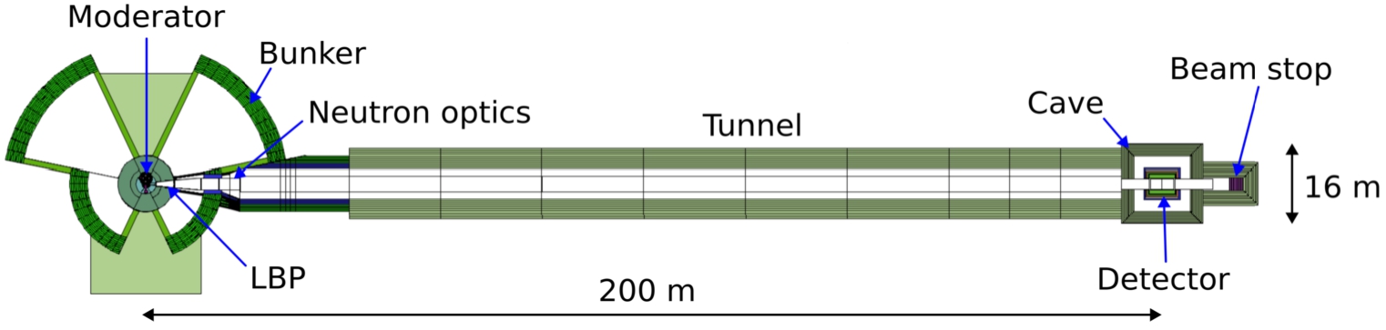
Figure 1 provides an overview of the experiment, which is also described below, together with, where appropriate, a short discussion on design choices.
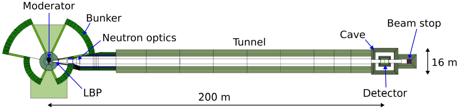
(1) Neutrons are passed into a beamline via the LBP. The
(2) A neutron mirror configuration is then used to focus the neutrons towards a distant carbon target. Various nested mirror systems were investigated using the neutron ray-tracing simulation, McStas [196]. Realistic physical constraints from the LBP and beam pipe shape were considered. The most promising optics option is a planar nested mirror system followed by a section of beampipe with a square cross section, which can deliver a FOM of 300 ILL units per year at 2 MW.
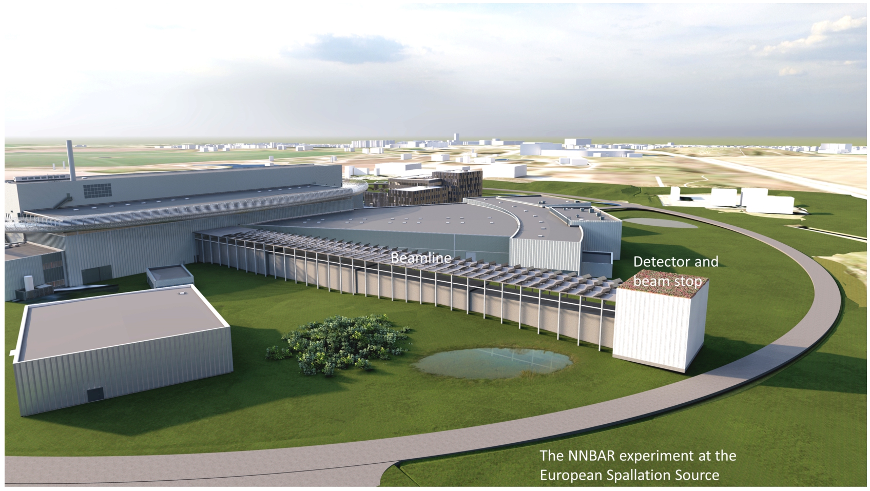
(3) The neutrons move out through the shielded bunker region into the NNBAR tunnel. Magnetic shielding surrounds the neutron path from the LBP up to the detector region. The ‘field-free clock’ of a neutron starts ticking when the particle enters the magnetic shielding region and is reset should the neutron be scattered e.g. in the optics system. The magnetically shielded region corresponds to a distance of around 200 m. A larger distance can potentially provide a higher sensitivity. However, physical limitations (the presence of a road, as seen in the cover picture of this volume) prevent a longer beamline.
A two-layer octagonal mumetal magnetic shield with additional active compensation was designed with the finite element method code, Comsol. This is largely a scaled-up version of a proven concept used for an atomic fountain [197]. With the magnetic shield, the field can be kept to values below 5–10 nT. For such a low field, the neutrons are quasi-free and optimising the experiment to maximise the FOM is thus appropriate.
(4) Biological shielding of the full beamline to match ESS safety standards was calculated using the MCNP radiation transport code [109], together with the Comblayer toolkit [30] for building geometric models. This was also an important study in showing that the performance of other beamlines would not be affected by radiation from NNBAR.
(5) Beyond radiation emission, the NNBAR beamline must fit within the engineering and physical constraints of the ESS infrastructure. A civil engineering study took place to quantify topics as diverse as floor loads and interference with the ESS instrument suit.
(6) An annihilation target sits near the end of the beamline. This is foreseen to be made of carbon and with a thickness of 100 μm. The target is a circular disk of radius 1 m. Varying this size changes both the FOM and, as is shown in this paper, the experiment cost. With a 1 m radius, the goal of a factor
(7) The annihilation detector sits in the shielded detector cave and surrounds the carbon target. The detector comprises time projection chamber (TPC) tracking, a scintillator and lead-glass calorimeter, and an active (scintillator) and passive (steel) cosmic veto. The detector measures the products from an antineutron-nucleon annihilation. The signature is a multi-pion state of invariant mass up to 1.9 GeV. TPC tracking was chosen as it provides 3-dimensional tracking, has good particle identification through continuous energy loss
(8) The bulk of neutrons would pass through the carbon target and eventually hit a beam stop made of neutron absorbers and moderators: B4C, polyethylene, steel and concrete. As for the carbon target, background from the beam stop forms a small part of the low energy particle flux into the detector.
(9) Considering the relative efficiencies of the ILL and NNBAR detectors and a three-year running time for NNBAR, a performance of around 1100 times the capability of the ILL experiment can potentially be achieved should the ESS with an accelerator power of 2 MW. This is more than doubled if the power is 5 MW. Furthermore, a parametric costing model was used which shows how the performance can be enhanced or reduced depending on the beam pipe size.
A summary of design parameters is given in Table 2.
Table 2
NNBAR design parameters
| Design parameter | Choice/value |
| Beam pipe radius at detector | 1 m |
| Magnetic field in shielded region | <5-10 nT |
| Magnetically shielded length | ∼200 m |
| Square-shaped tube length | 20 m |
| Optical system | Monoplanar |
| Annihilation detector | TPC (tracker) |
| Scintillator/lead-glass (calorimeter) | |
| Scintillaror (active cosmic veto) | |
| Steel (passive cosmic shield) | |
| Annihilation detector efficiency | 68% |
| Background events | ∼0 |
| Fast neutron rejection efficiency loss | 7% |
| Loss due to non-zero magnetic field | 5% |
| Running time | 3 yr |
| FOM (ILL units) | 1100 (2 MW) |
| 2700 (5 MW) |
This paper also points towards future work. In particular, experiments on detector prototypes and a smaller-scale NNBAR, such as HIBEAM, can be used to test and optimise simulations. A dedicated study on detector granularity and beamline optimisation in the detector area can quantify and suppress the influence of low energy beam-related particles. A further civil engineering study is required to guarantee that the NNBAR beamline does not interfere with neighboring beamlines or other ESS facilities.
4.Theoretical background
This section describes the motivation for searching for
4.1.Neutron–antineutron oscillations as a key observable of baryon number violation
It can be strongly argued that baryon number is not expected to be conserved. Baryon number violation is one of the so-called Sakharov conditions [159], necessary for a theory of baryogenesis to explain the origin of the observed matter-antimatter asymmetry. Furthermore, like lepton number (
It should also be noted that, notwithstanding the conservation of
It should also be noted that the existence of sphaleron processes at the electroweak scale implies that a baryon asymmetry produced at a higher scale by, e.g. a (
Given the above arguments, it is no surprise that the phenomenon of
A theory-agnostic and exploratory approach to BNV searches also highlights the need to search for
The
4.2.Estimating neutron–antineutron oscillation rates
In an effective field theory approach, the
Calculations for
4.3.Neutron–antineutron oscillations and post-sphaleron baryogenesis
As the
Figure 2 shows the scalar mass scale as a function of the
![Likelihood distribution for neutron–antineutron oscillation time for a PSB scenario. The limit from Super-Kamiokande (SuperK-2) [6] is shown. Figure adapted from reference [36].](https://content.iospress.com:443/media/jnr/2023/25-3-4/jnr-25-3-4-jnr230951/jnr-25-jnr230951-g003.jpg)
4.4.Neutron–antineutron oscillations and the origin of neutrino mass
Another open question which
4.5.Other scenarios of neutron–antineutron oscillations
A range of extensions of the SM, beyond those described in the aforementioned sections, predict observable
Fig. 3.
Relationship between the oscillation time and the mass scale for new physics in a R-parity violating supersymmetry scenario. The calculations are presented using the best estimate for the matrix element together with two predictions corresponding to shifting the matrix element according to uncertainties thus forming an uncertainty envelope around the central estimate. The limits on oscillation time from searches at the ILL (ILL-1994) [44] and Super-Kamiokande (SuperK-1 [4] and SuperK-2 [6]) are shown. Figure adapted from reference [74].
![Relationship between the oscillation time and the mass scale for new physics in a R-parity violating supersymmetry scenario. The calculations are presented using the best estimate for the matrix element together with two predictions corresponding to shifting the matrix element according to uncertainties thus forming an uncertainty envelope around the central estimate. The limits on oscillation time from searches at the ILL (ILL-1994) [44] and Super-Kamiokande (SuperK-1 [4] and SuperK-2 [6]) are shown. Figure adapted from reference [74].](https://content.iospress.com:443/media/jnr/2023/25-3-4/jnr-25-3-4-jnr230951/jnr-25-jnr230951-g004.jpg)
Neutron oscillations also feature in extra-dimensional models. One such type of model [103,145] gives an example of how proton decay can be strongly suppressed but
Extensions of the SM with scalar fields give rise to
4.6.Free and bound neutron–antineutron conversions
The Schrödinger equation for the evolution of an initial beam of slow-moving neutrons which can convert to antineutrons after a time t is shown in Equation (2).
The term
Here
It can thus be seen that the conversion rate becomes suppressed when the neutron and antineutron are no longer degenerate in energy. For neutrons bound in nuclei, values of
With magnetic shielding such that the average magnetic field is less than around 5–10 nT for an experiment with cold neutrons, the so-called quasi-free regime (
From this equation it becomes clear that the FOM defined in Equation (1) approximates the number of antineutrons arriving at the annihilation detector region at a given experiment for a specific value of oscillation time. The FOM is thus a proxy for an experiment’s discovery potential.
Neutrons bound in nuclei belong to the region:
Unlike Equation (4), Equation (5) retains the
4.7.Antineutron-nucleon annihilation
The composition and properties of the visible final state produced following an extranuclear
A model of
Table 3 shows the simulated and measured particle multiplicities (M) and the total energy of final state particles, produced after
Table 3
Average particle multiplicities (M) compared between data and simulation. From reference [15]
| —– | —– | ||||||
| 4.60 | 1.22 | 1.65 | 1.73 | 1762 | 0.96 | 1.03 |
5.Searches for neutron–antineutron oscillation
This section describes ways in which
5.1.Cosmological and astrophysical implications of neutron oscillations
There is limited sensitivity from cosmological and astrophysical measurements to the free
5.2.Searches with free neutrons in a beam
Neutrons are cooled in a moderator and then passed to a system of neutron optics. The neutron beam is focused across a propagation region. Neutron focusing is important as interactions between the propagating neutron and the guide wall can ‘reset the oscillation clock’.22 The neutron’s flight path must be magnetically shielded such that the field should be less than 5–10 nT. Near the end of the propagation region there is a detector can observe the products arising from the annihilation of an antineutron in a thin target. A beam stop is placed behind the detector region. The whole experiment must be biologically shielded.
Free neutron searches using beams have been made at the Pavia Triga Mark II reactor [67,68] and at the ILL [44,95]. The final ILL search [44] gave a limit on the free neutron oscillation time of
5.3.Searches with bound neutrons
Searches have also been made with bound neutrons at large mass detectors. Such searches look for a signature of pions and photons arising from a
Limits on conversion times for neutrons bound in nuclei (
Super-Kamiokande has provided the current most competitive inferred limit on the free neutron conversion time. This is based on a putative
5.4.Searches with ultracold neutrons
In addition to the above searches, it has been proposed to use ultracold neutrons (UCNs) in a material trap [119,125,127]. This offers the possibility of potentially cheaper experiments than one using beam neutrons as long propagation distances are not needed. However, this approach has its own drawbacks as, for a large volume tank, the UCN free flight time is around 1 s. A possible search at the WWR-M reactor has been considered [96,97,172]. The sensitivity would be lower by more than an order of magnitude than for NNBAR.
5.5.Comparison of limits and sensitivities
Figure 4 shows limits on conversion time which have so far been achieved with bound and free neutron searches. A new generation of large mass detectors at DUNE [11,12], Hyper-Kamiokande [3,5] and JUNO [14,88] has the potential to substantially extend sensitivities. The projected sensitivity for the future DUNE experiment [12] is shown. The sensitivities of the future Hyper-Kamiokande and JUNO experiments are not yet published.
Fig. 4.
Limits from searches with bound neutrons (blue circles) and free neutrons (red circles) and the sensitivity of the future DUNE (blue triangle) experiment.
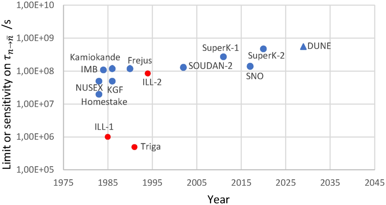
It should be emphasised that both types of searches (free and bound) are needed. Any comparison between limits from free and bound neutron searches relies on model assumptions, such as
6.Software
In order to calculate the sensitivity of the
Fig. 5.
Above: an illustrative overview of the essential components required for the NNBAR experiment. Below: a simulation flowchart outlining the simulation and optimization of the NNBAR experiment. MCNP simulations of the ESS lower moderator are used as starting point. The focusing of cold neutrons is studied using McStas while the background stemming from faster neutrons is investigated using MCNP. Finally, GEANT4 is used for the detector simulation. The MCPL format is used to exchange data between the different simulations. Figure from reference [47].
![Above: an illustrative overview of the essential components required for the NNBAR experiment. Below: a simulation flowchart outlining the simulation and optimization of the NNBAR experiment. MCNP simulations of the ESS lower moderator are used as starting point. The focusing of cold neutrons is studied using McStas while the background stemming from faster neutrons is investigated using MCNP. Finally, GEANT4 is used for the detector simulation. The MCPL format is used to exchange data between the different simulations. Figure from reference [47].](https://content.iospress.com:443/media/jnr/2023/25-3-4/jnr-25-3-4-jnr230951/jnr-25-jnr230951-g006.jpg)
An overview of the simulation chain used to construct a comprehensive model of the NNBAR experiment is given in Fig. 5. This simulation chain consists of multiple components, each dedicated to specific aspects of the experiment. It effectively tracks the path of neutrons as they are focused and propagate towards the annihilation detector. The first step is the simulation of the neutron source as described in Section 2 in Reference [161]. Following this, several different simulations are necessary depending on the particle energy. The reflection and focusing of cold neutrons is modelled using McStas [196]. The low magnetic field region is designed and optimized using the finite-element simulations tool COMSOL [81,82]. The propagation of fast neutrons is simulated using MCNP [108] or PHITS [166] in order to determine the required beamline shielding as well as their contribution to the experiment’s radiation background. The MCPL format [128] is used to exchange particle trajectories between the different tools.
The annihilation detector, which observes the multi-pion final state of the annihilation of antineutrons on the carbon foil target must also be modeled. This simulation relies on GEANT4 [20], a standard simulation toolkit widely employed at particle physics experiments for detector simulations. The annihilation events are generated using a simulation tool that assumes an initial antineutron interacting with a carbon nucleus [48,50,106]. The detector modeling also requires the simulation of backgrounds, such as fast spallation products interacting with the foil, and external backgrounds, such as those arising from cosmic rays. The cosmic ray particles are generated using the Cosmic-ray Shower Library (CRY) [113].
In addition to the GEANT4 full simulation used for the analyses, parameterizations of the detector subsystems were also developed and employed in some cases to provide a fast estimate of the detector response and to cross-check the results obtained from the full simulation.
7.The ESS and a new moderator
Details of some of the infrastructure necessary for NNBAR can be found in the first volume of the HighNESS CDR [161]. Section 1 of that document gives an overview of the ESS. The design of a
8.The NNBAR beamline
Following their production in the moderator, the neutrons undergo extraction via the LBP, as detailed in Section 1 of Reference [161]. These neutrons are then directed and focused toward the annihilation target, located at a distance of 200 m from the neutron source.
The LBP holds a central and indispensable role in the NNBAR experiment. Without this infrastructure, the experiment’s sensitivity objectives could not be reached. The LBP is strategically designed to occupy the equivalent space of three standard ESS beam ports. The physical dimensions of the LBP undergo a gradual increase in size as it extends from a modest area of
The LBP serves not only to transport cold neutrons for use in the NNBAR experiment through the target monolith but also leads to a substantial increase in radiation outside of it. Consequently, the NNBAR beamline require additional shielding to handle the increased dose rate compared to a standard ESS beamline. To determine the necessary amount of shielding, simulations of the entire NNBAR beamline, including the experimental cave and the beam stop, were conducted using the radiation transport code MCNP [108]. A detailed beamline model of the NNBAR beamline was constructed for these simulations using CombLayer [30]. The CombLayer software package allows the construction of geometry models in C
The complete simulation of a beamline, even in the case of a beamline like NNBAR, is computationally expensive. To make these calculations feasible, the simulation of the beamline was split up in separate simulations of different sections of the beamline. For each of these sections, inputs were generated using the duct source method [87], a standard variance reduction method for long beamlines. However, the unique characteristics of the LBP necessitated the development of a dedicated duct source method. Unlike most regular beamlines at ESS and other neutron facilities, where the neutron distribution can be reasonably assumed to be uniform over the area of their beam port, the large size of the LBP precludes such an assumption. Consequently, when generating the simulation input, it was essential to account for the correlations between neutron position, direction, and kinetic energy.
The coordinates of particles coming from the moderator were sampled to reproduce the distribution at 2 m from the source. The particles were then assigned momenta following the duct source method and kinetic energies following a uniform distribution. Finally, each of these tracks was assigned a particle weight based on the probability density function calculated from their position, momentum and energy in order to reproduce the original distribution [116]. All the beamline calculations presented in this section were made using this methodology.
Only the radiation doses caused by neutrons were calculated for the results presented in this section. Doses from other particles, e.g. gamma-rays, will be evaluated in the future. However, neutrons are expected to be the dominating source of radiation from the LBP and the NNBAR beamline so the shielding solutions presented here should be still be sufficient when taking other types of radiation into account.
8.1.NNBAR beamline simulation in the bunker area
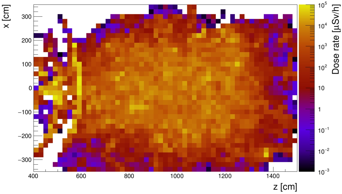
Fig. 6.
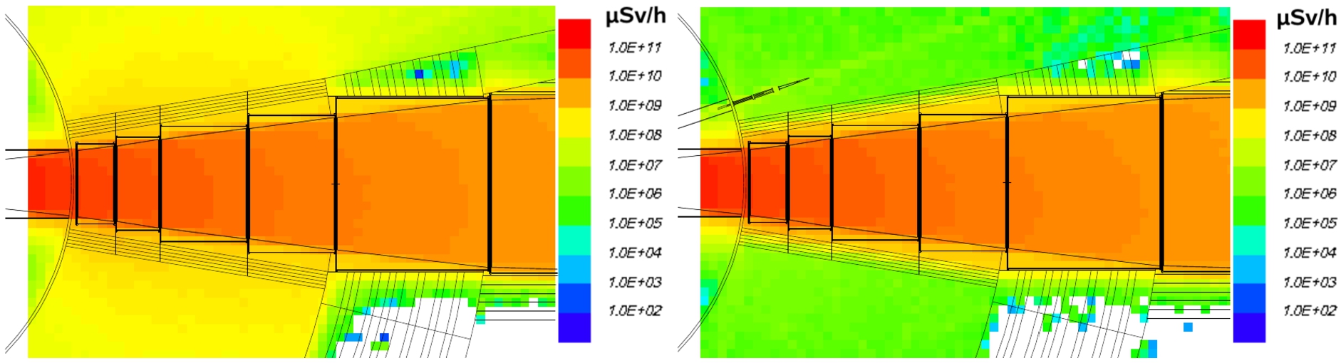
Radiation dose map of the inside the bunker close to the LBP. Left: radiation dose map without additional shielding. Right: dose map with 40 cm thick walls of heavy concrete around the NNBAR beamline.
The ESS bunker wall was designed with the objective of reducing the radiation dose outside it to a level below the threshold defined with respect to the supervised area at the ESS [189]. This threshold is set at
The current design of the bunker wall achieves this target value for the parallel use of 22 standard ESS beamlines at 5 MW without the need for shielding inside the bunker. However, in the case of the NNBAR experiment, due to the size of the LBP, shielding inside the bunker will be necessary. This is illustrated in the left panel of Fig. 6 which shows a neutron dose map of the bunker interior. The resulting dose in the vicinity of the beamline exceeds 100 Sv/h, several orders of magnitude higher than is expected from regular ESS beamlines.
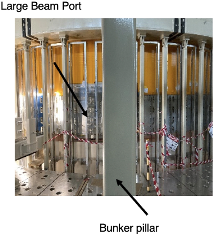
The right panel shows the situation when the beamline is surrounded by 40 cm thick walls of heavy concrete. The dose outside the shielding is reduced by two orders of magnitude and is similar or somewhat lower than a standard ESS beamline. In Fig. 6 above the LBP, the first part of the guide for the HEIMDAL beamline is depicted. As can be seen, the additional shielding effectively reduces the background dose generated by the LBP to a level below that produced by HEIMDAL. Thus, it is evident that the dose has been reduced to a sufficient extent, allowing the bunker walls to shield it below the specified limit.
Fig. 7.
Dose map of the top of the existing ESS bunker roof when running the LBP.
The requirements for the bunker roof differ from those for the wall. Since personnel will not be working regularly on the roof, the established dose limit criteria by the ESS are slightly higher than those for the bunker wall. The limit is set at 25 μSv/h though, after applying a safety margin, this reduces to 12.5 μSv/h. A further factor taken into account for the design of the bunker roof is the dosage in other areas, such as the ESS main office building, due to skyshine. The limit for the dose received due to skyshine is 100 μSv/y [200]. Once again, the design of the bunker roof was selected to meet these limits when operating with the complete set of regular ESS beamlines. However, in the case of NNBAR, it will be necessary to add extra shielding in the area near the LBP. Figure 7 illustrates the situation without any additional shielding. The average dose on top of the roof directly above the LBP is calculated to be 3.3(4) mSv/h. A conservative empirically based estimate of the resulting skyshine can be made using Equation (7).
Fig. 8.
Dose map of the top of the existing ESS bunker roof with additional shielding of the LBP. Left panel: additional shielding of 70 cm inside of the bunker. Right panel: additional shielding inside the bunker (70 cm of steel) and on top of the roof (40 cm of heavy concrete).
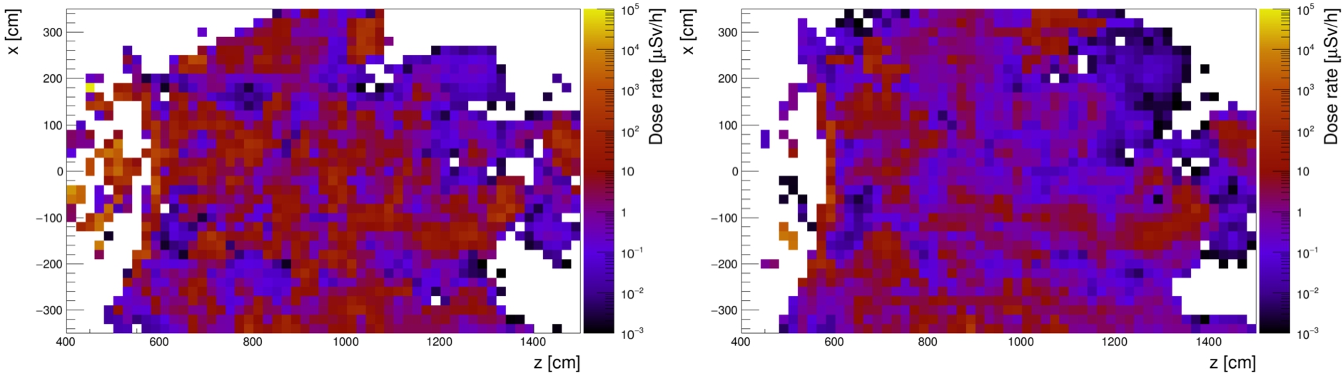
The current study only investigated cases in which the existing roof itself is not modified. This leaves two options to add shielding to the bunker roof. The shielding can be added inside the bunker or on top of the existing roof. The size of the NNBAR beamline leaves space to add 70 cm of shielding material between the vacuum pipe and the bunker ceiling. In the current simulation, steel was chosen as material for this additional interior shielding. The left panel of Fig. 8 shows the dose map on top of the roof with this addition. The average doses are reduced to 16(2) μSv/h and the skyshine, calculated using Equation (7), to 8.5(9) μSv/y. This is at the edge of the dose limit criteria.
The right panel of Figure shows the dose map when also adding 40 cm of heavy concrete on top of the current bunker roof. The average dose is 5.0(7) μSv/h and the skyshine 2.6(4) μSv/y. While more detailed studies are required, this seems sufficient to fulfill the ESS dose limits. Further studies need to be conducted to fully assess how to integrate this additional shielding into the bunker structure. Additionally, a discussion of the possible inclusion of shutters in this area should be undertaken. This is discussed in Section 19.1.
8.2.The NNBAR tunnel
Fig. 9.
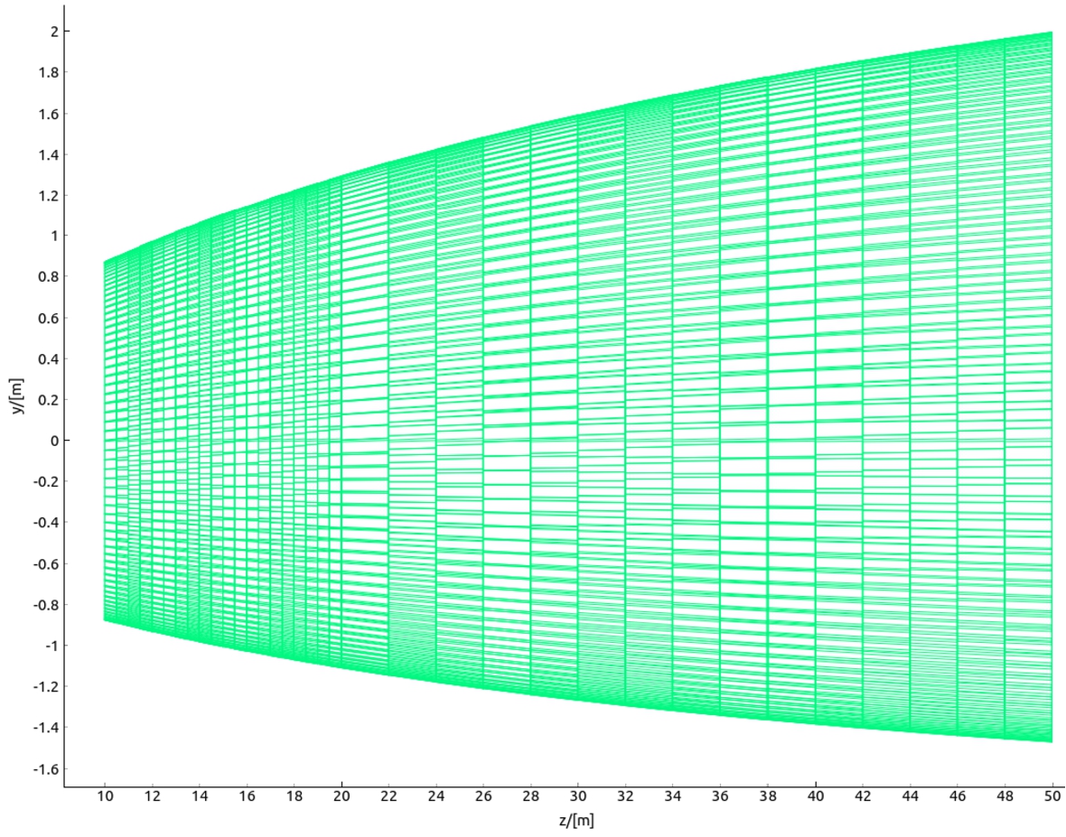
Detailed view of the CombLayer model of the NNBAR experiment for the region from the bunker wall until the exit of the experimental hall.
The construction of the NNBAR experiment implies the installation of a feed-through in the bunker wall, as well as the creation of an opening large enough to accommodate the NNBAR vacuum pipe and the magnetic shielding structure (see Section 11). Biological shielding must be sufficient such that the specified dose limits for the supervised area are not exceeded. The vacuum pipe has a rectangular cross section of 2.4 m × 2 m up to 18 m from the moderator. After this, the pipe has a circular cross section with a radius of 1.5 m. It is worth pointing out that existing instruments and infrastructure within the ESS instrument hall impose constraints on the dimensions of the shielding.
The model of the tunnel used in the simulations is shown in Fig. 1. Figure 9 provides a more detailed view of the region extending from 10 to 50 m from the moderator. The initial 25 m, starting from the bunker, remain within the confines of the D03 experimental hall (as shown in Fig. 7 of Section 1 of Reference [161]). Within this zone, the NNBAR tunnel’s wall configuration comprises 1 m of steel backed by 1.5 m of heavy concrete. This design was chosen to minimize interference with existing structures and adjacent experiments, notably the LOKI experiment located to the south of the NNBAR experiment. After leaving the bunker, the tunnel widens, providing both room for the magnetic shielding of the beamline and facilitating access to the tunnel for tasks such as vacuum maintenance.
Fig. 10.
Dose map of the NNBAR tunnel.
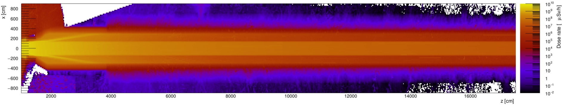
Beyond the D03 experimental hall, there are fewer space constraints, allowing for the use of regular concrete as the wall material. In the simulations, a uniform wall thickness of 4 m was initially employed for the entire tunnel. However, the simulation results indicate that this thickness is not required along the entire length.
Figure 10 illustrates the dose map of the NNBAR beamline from the bunker wall up to 175 m away from the source. The dose rate remains below the limit of
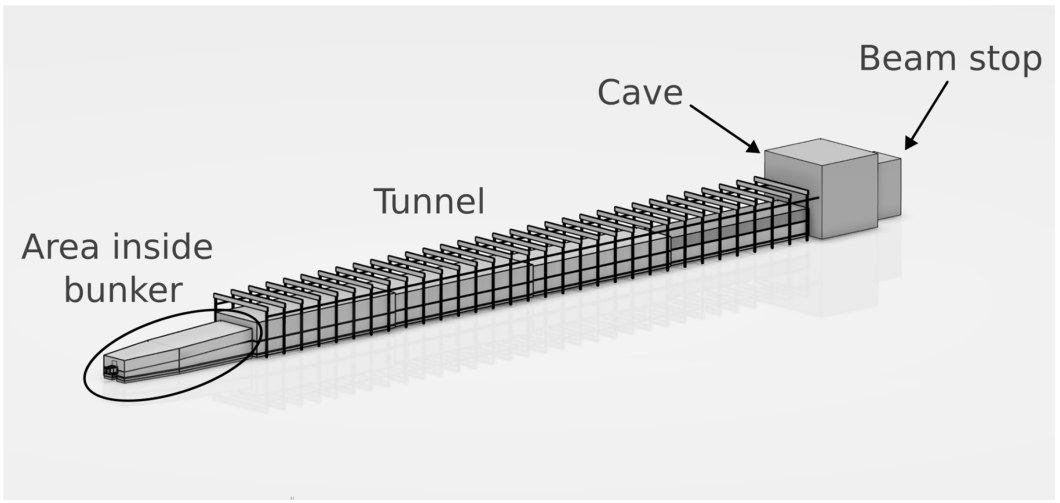
The shielding dimensions presented in this section have formed the basis of a CAD model of the NNBAR beamline. The model includes the area inside the experimental hall, the tunnel, experimental cave and beam stop. An overview of the model is shown in Fig. 11.
Fig. 11.
CAD model of the NNBAR beamline.
8.3.The interface between the NNBAR beamline and the instruments gallery
A particular challenge in designing the shielding for the NNBAR tunnel is the presence of the already existing instrument gallery located beneath the D03 building, as shown in Figs 12 and 13. The instrument gallery serves the purpose of housing supporting equipment such as ventilation systems and instrument-related pipes. Notably, the gallery intersects with the planned tunnel approximately 30 m from the moderator, takes a turn, and then runs parallel to the tunnel for approximately 25 m. The gallery has a roof made of 55 cm of regular concrete, which will require replacement and reinforcement. Additionally, to ensure adequate shielding, extra measures will be necessary in front of the gallery. This is discussed further in Section 19.1.
Fig. 12.
The instrument gallery located at the exit of the D03 building.
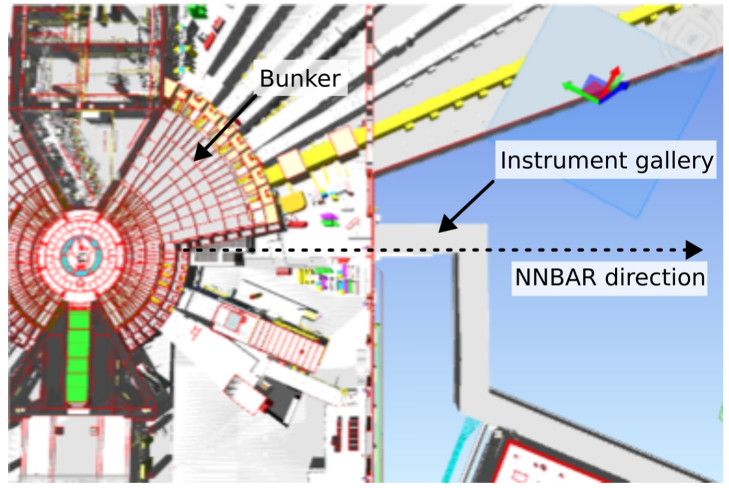
Fig. 13.
The interface between the NNBAR beamline and the ESS instrument gallery (circled in red).
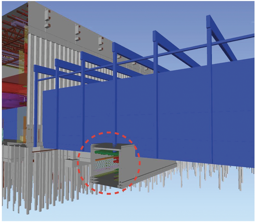
Fig. 14.
Dose maps for the NNBAR beamline and D03 instrument gallery for different shielding options. The investigated geometry is shown in the top row, the middle row shows the respective dose map, and the bottom row gives a projection of the dose map directly below the ceiling of the gallery for the respective geometry.
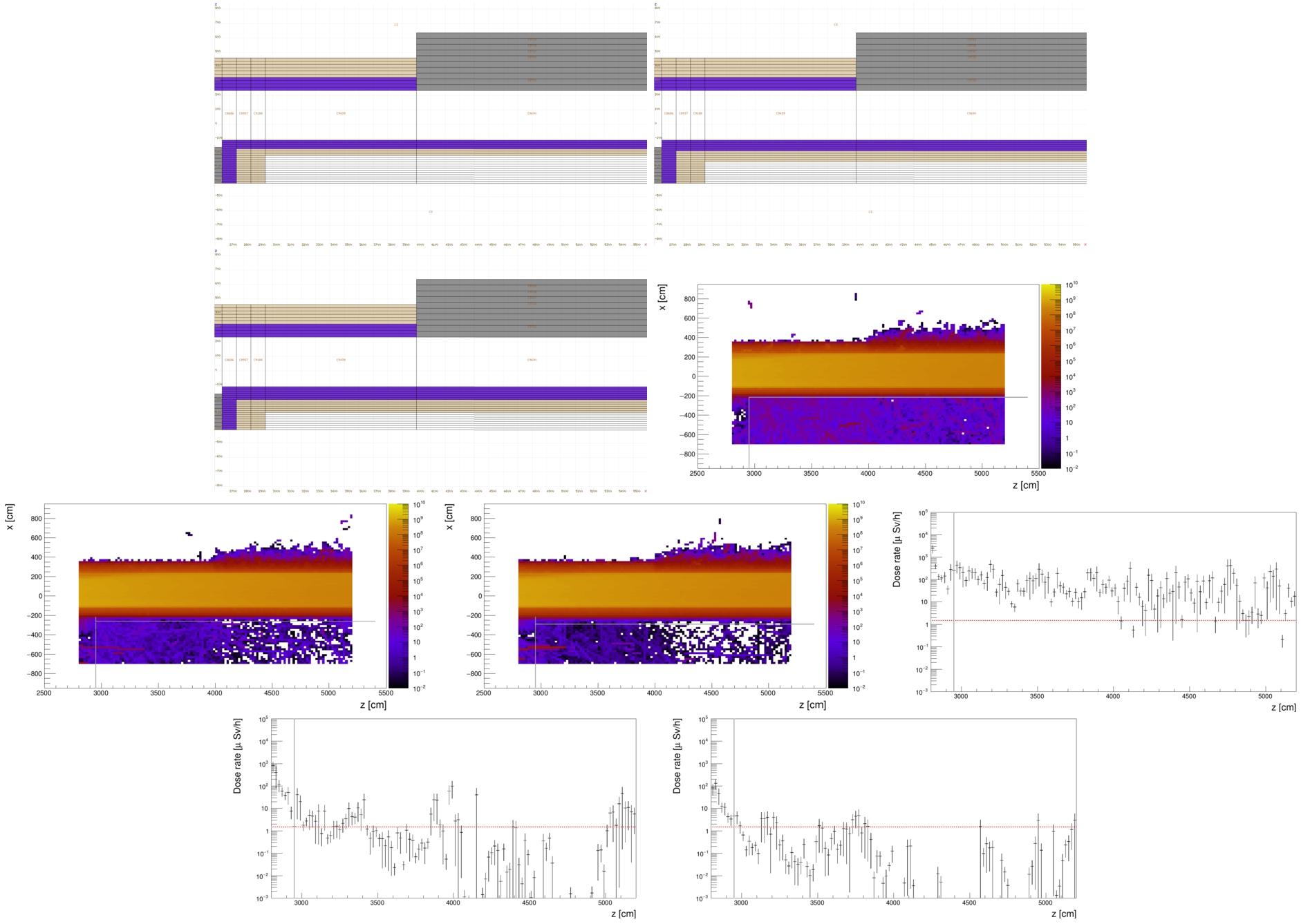
Different options for the gallery shielding are summarized in Fig. 14. In the left panels, while the gallery roof has been replaced, the dimension of the gallery has been kept the same and only the space available between the gallery and the NNBAR beamline has been used for additional shielding. In total, 105 cm of shielding have been placed above the gallery comprising 60 cm steel and 45 cm of heavy concrete. This is not sufficient to create a safe working environment, with the dose just below the ceiling of the gallery exceeding
8.4.The NNBAR cave and beam stop
Fig. 15.
Model of the NNBAR cave and beam stop.
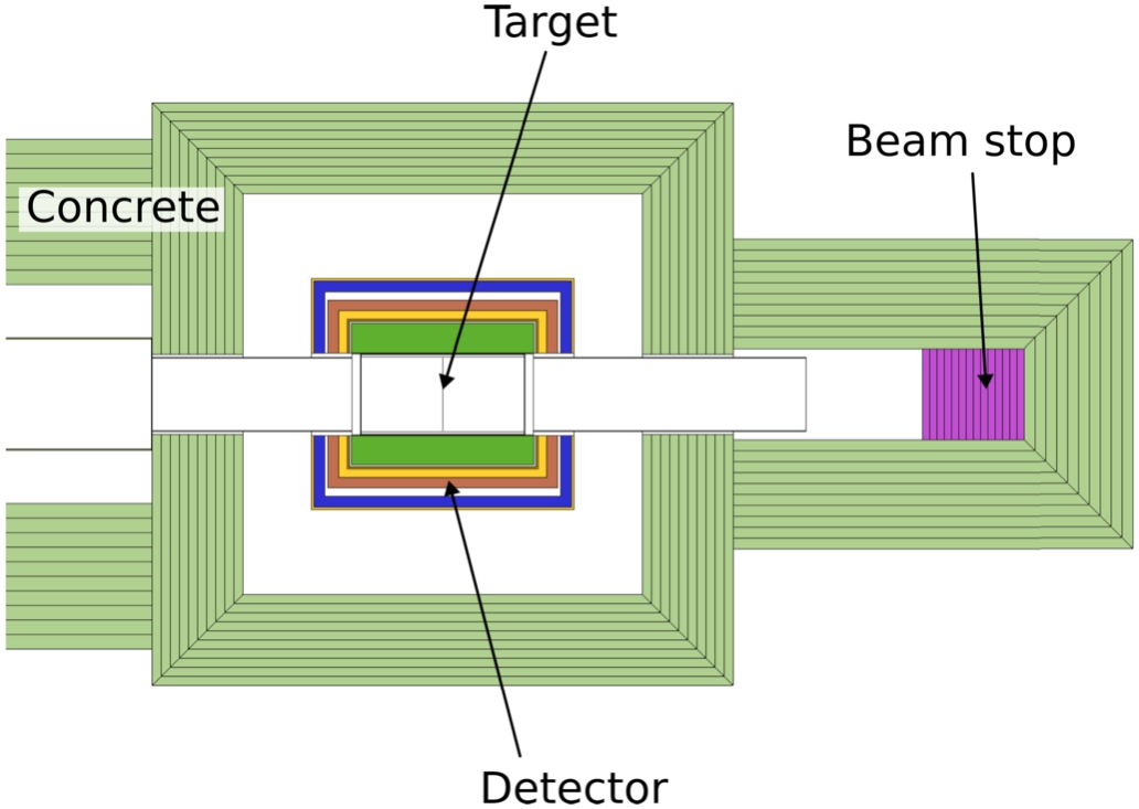
At the end of the NNBAR beamline, the annihilation target and the annihilation detector (as described in Section 13) will be positioned. This equipment will be housed in an experimental hall referred to as the ‘NNBAR cave’ (see Fig. 15). Within this hall, not only will the detector be situated, but it will also accommodate auxiliary electronics and support structures. The NNBAR cave will receive the full NNBAR beam and thus necessitate robust shielding and a beam stop to safely terminate the beam.
In the current model, the front wall of the NNBAR cave is located at a distance of 192 meters from the moderator. At this point, the beamline’s radius reduces from 1.5 m to 1.0 m. Importantly, the thickness determined for the far end of the tunnel (250 cm concrete or 175 cm heavy concrete) will also meet the ESS dose requirements for a supervised area. The beam stop will be positioned approximately 10 to 15 m from the annihilation target and is responsible for absorbing the entire neutron beam that travels down the NNBAR beamline. Therefore, it must have a diameter at least as large as that of the beamline itself. Various material combinations and thicknesses have been explored for the beam stop.
Fig. 16.
Left: dose map of the NNBAR cave and beam stop. Right: projection of the dose map at the center of the beam stop.
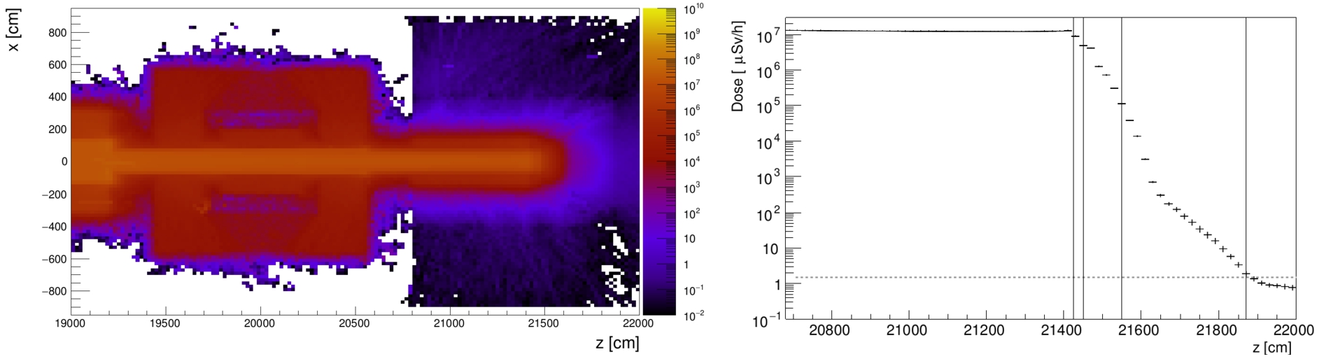
In Fig. 16, a dose map is presented for a beam stop configuration comprising a thin top layer (0.5 cm) of B4C, supported by 25 cm of polyethylene, 100 cm of steel, and 320 cm of concrete. The projection illustrates that this configuration is effective in reducing the dose to below
9.Civil engineering aspects of the NNBAR experiment
The construction of the NNBAR beamline will require a redesign of some parts of the existing facility that may interfere with the proposed beamline. In order to understand the extent of potential interference between NNBAR and ESS infrastructure and evaluate associated construction work, a civil engineering project was conducted as part of the HighNESS project. This project was a collaborative effort involving the NNBAR team, the ESS Facility Management division (FM), and the SWECO company [193]. It aimed to determine the required length of the NNBAR beamline, assess its structural requirements, and analyze factors such as width, height, and force loads related to shielding and surrounding structures.
9.1.Modifications to the bunker area and the D03 instrument hall
The first 15 m of the NNBAR beamline will be placed inside the neutron bunker (see Section 1 of Reference [161]) in the position currently occupied by the ESS Test Beamline. This beamline will be used in the early days of the ESS project to characterize the neutron source but could later be moved to a different location to allow the construction of the NNBAR experiment. The significantly larger size of the NNBAR beamline will introduce interference with the existing steel structure supporting the bunker roof as shown in Fig. 17.
Fig. 17.
Interference between the bunker steel structure and the NNBAR beamline.
This problem may find a solution as the steel structure is planned to undergo significant modifications. These modifications are necessary due to the additional shielding requirements for the bunker roof, driven by the radiation contribution from the NNBAR beamline (see Section 8.1). Additionally, modifications to the north sector bunker wall (see Section 1 of Reference [161] for an explanation of the ESS sectors) will be required to accommodate a sufficiently large feed-through.
Beyond the bunker, the subsequent 21 meters of the beamline will be situated within the experimental hall of the D03 building. The existing concrete slab of the building has a load capacity of 14 t/m2 (10 t/m2 close to the facade) which will prove inadequate to support the heavy load required for the beamline shielding, as discussed in Section 8.2. Consequently, the reinforcement of the floor will be necessary. This entails the addition of an extra distribution slab, measuring 750 mm in thickness towards the west sector and 1250 mm for the north sector section outside the bunker area as shown in Fig. 18.
Fig. 18.
Proposed floor reinforcement solution for the NNBAR beamline for the D03 area.
Furthermore, the length of the beamline makes it necessary to cross the already existing D03 building facade. Given the substantial height and width of the NNBAR beamline and its shielding, it is likely that modifications to the anti-seismic steel structure frame and a section of the building foundation will be necessary. This is because one of the building pillars is situated in the path of the new beamline. However, it should be pointed out that the structure has been designed to accommodate the accidental removal of any of these individual columns. This was achieved by designing the truss structure to span a double bay, allowing for the accidental removal of one of the columns in the experimental hall. This design ensures that the structure is robust enough to withstand unforeseen events, such as the loss of a column due to incidents like a vehicle collision or a swinging crane load. Furthermore, this design approach offers a degree of future flexibility, as it allows for the intentional removal of one of the columns during structural alterations, as would be the case with the NNBAR beamline. In such a scenario, it will be necessary to reinforce the columns, crane beam, brackets supporting the crane beam, and the walkway support beams on adjacent columns (typically two or four). An independent analysis should assess the feasibility of this undertaking.
9.2.The area outside the D03 instrument hall
Fig. 19.
Interference between the NNBAR beamline and the ESS circular road for a beamline of length 300 m.
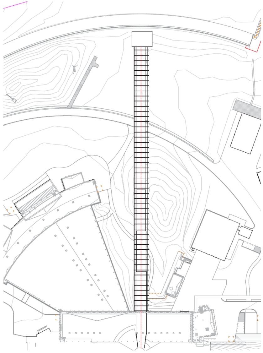
The proposed NNBAR beamline has a total length of 200 m, with approximately 160 m extending outside the D03 building before reaching the NNBAR cave (see Fig. 12 of the HighNESS CDR Volume I). While the optics studies in Section 10.9 determined that the 200 m design provides the best trade-off for experiment sensitivity, this section examines the implications of a longer beamline from a civil engineering perspective. As depicted in Fig. 19, an extension of the beamline beyond 200 m would imply intersecting with the circular road encircling the ESS area, necessitating a rerouting of the road. When considering the circular road as a boundary, a detailed analysis of the area near the NNBAR beamline confirmed that there are no conflicts between the beamline foundation and local utilities or subservices. However, a more thorough analysis is required to assess whether local modifications to the foundation are needed to support the loads of the shielding and the instrument cave. Furthermore, an investigation into the necessity of downward shielding to ensure the safety of subservice contents is pending. Nonetheless, given that the subservices are situated at a substantially lower level than the instrument gallery, as discussed in Section 9.3, it is very likely that this is not a significant concern.
Fig. 20.
Different options for the NNBAR tunnel structure. A: shielding without weather protection and a crane vehicle. B: shielding and traverse-crane with roof. C: shielding, traverse-crane and full weather protection.
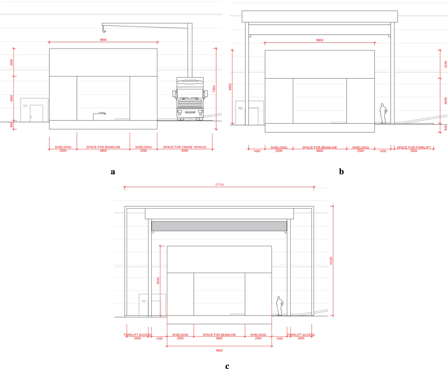
As presented in Section 8, the necessary shielding thickness outside the D03 hall depends on the chosen material and decreases over the length of the beamline. For regular concrete the required thickness ranges from 400 cm to 250 cm, while for heavy concrete, it ranges from 250 cm to 175 cm. The use of heavy concrete is associated with a higher cost of material. A further study of the structure surrounding the shielding resulted in three possible options, as illustrated in Fig. 20 using the dimensions for heavy concrete. Figure 20a depicts the simplest option, which consists of a shielding layer without any additional weather protection and an autonomous crane vehicle for moving shielding blocks. Further investigation is needed to determine whether it is feasible to leave the structure unprotected, as exposure to water and wind could lead to damage. This option would require the construction of a service road along the entire length of the beamline. Nevertheless, it is likely the most cost-effective option in terms of construction. The second option is shown in Fig. 20b, consisting of shielding and a traverse-crane going along the entire structure, with a simple roof structure as weather protection. This option would also require a service road, but not of the same magnitude as for the first option, as is it would not need to be adapted for such heavy vehicles.
Lastly, in Fig. 20c, you can see the configuration featuring shielding and a traverse-crane, all enclosed within full weather protection, effectively creating an annex-building connected to the D03 instrument Hall. To accommodate incoming truck or forklift vehicles, the internal communication pathways must be sufficiently wide. This solution offers the advantage of simplified communication between D03 and the NNBAR experimental cave through internal walkways. However, this construction imposes different requirements on installations, such as ventilation, electrical systems, and plumbing.
9.3.Interface between NNBAR and the instrument gallery
Fig. 21.
Position of the instrument gallery in relation to the beamline. The instrument gallery is shown in green and the beamline in red.
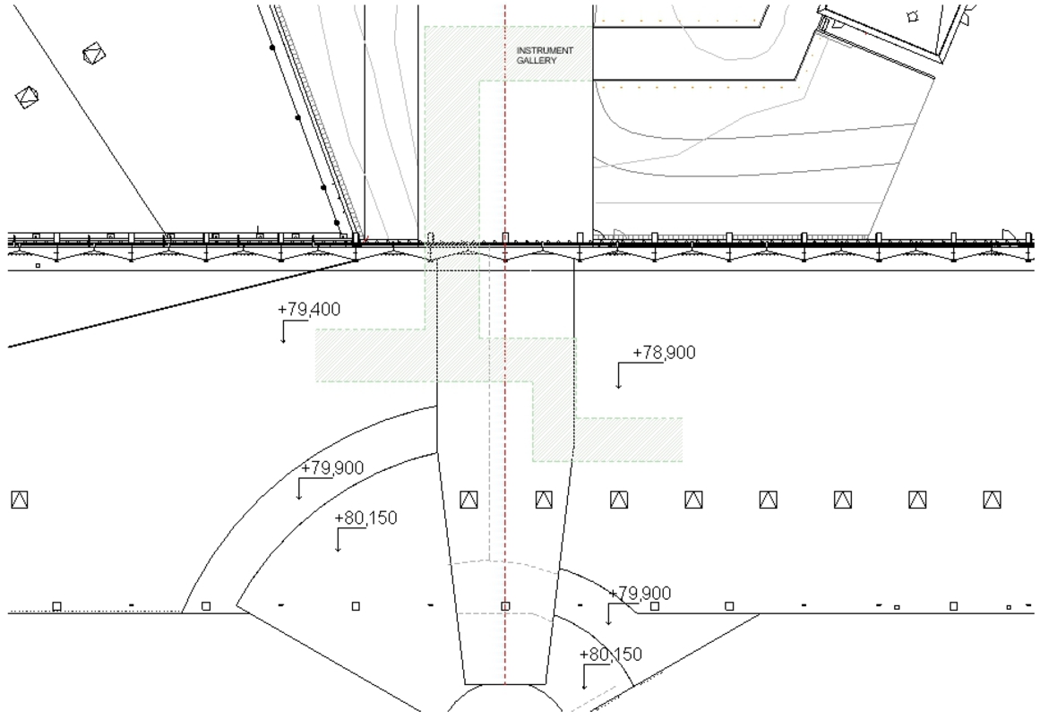
As discussed in Section 8.3 and illustrated in Fig. 13, the position of the instrument gallery intersects with the NNBAR beamline, resulting in overlapping structures at multiple points (see Fig. 21). This situation presents a complex engineering challenge, as it requires both shielding the instrument gallery from the radiation emitted by the beamline and managing the load transferred from the beamline to the gallery.
Fig. 22.
Position of the instrument gallery in relation to the beamline. The instrument gallery is shown in green and the beamline in red.
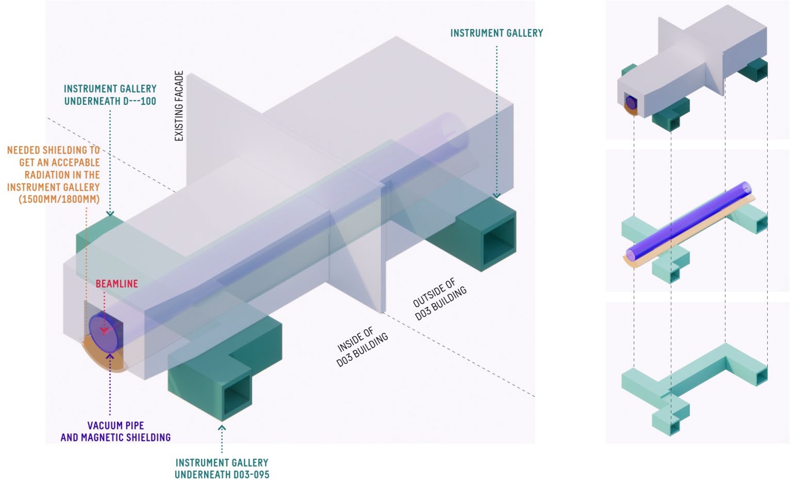
Fig. 23.
Interfaces between the instrument gallery and the NNBAR beamline. Conflicts are highlighted with circles.
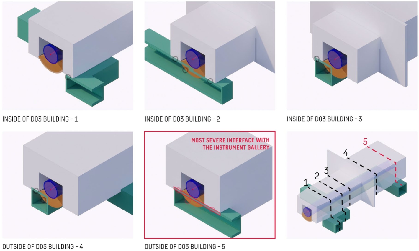
As was shown in Section 8.3, between 150 cm and 180 cm of shielding material (half steel, half heavy concrete) is required to reduce the radiation from the NNBAR beamline to an acceptable level in the instrument gallery. Figure 22 shows a 3D-sketch of the beamline (purple) and the gallery (green). The orange volume shows the space needed for the shielding. The pictures on the right side of Fig. 22 show the disassembled beamline, to give an impression of the relation between the instrument gallery and the beamline. It is clear that there is not enough space in between for the shielding. This is also illustrated in Fig. 23, where the interface between the gallery and the beamline is shown in five different positions. Circles highlight the conflicts between the two. This leaves two options, raising the beamline or adding shielding inside the instrument gallery which would require the rerouting of existing pipes.
Figure 23 highlights not only direct conflicts between beamline and gallery but also issues due to the load caused by the shielding. The study of how much load the instrument gallery can manage was conducted in parallel.
Fig. 24.
The current loads on the instrument gallery, which were the base for its design.
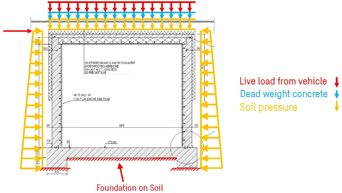
Fig. 25.
A: estimated loads from the NNBAR shielding. B: loads from the shielding in relation to the instrument gallery design loads.
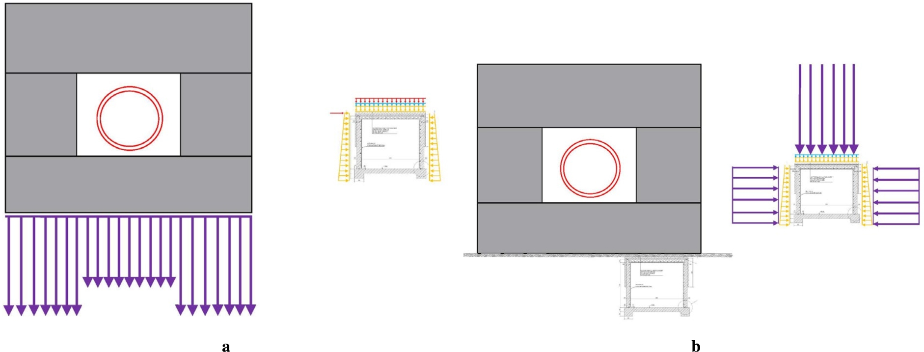
When the instrument gallery was initially designed, it was based on expected loads at that time, as shown in Fig. 24. Comparing this to the load produced by the NNBAR shielding in Fig. 25, it becomes evident that the additional load exceeds the gallery’s capacity. Consequently, the new construction around the beamline must be designed to support this additional load. The principle for solving the problem is illustrated in Fig. 26. A substantial beam, supported by drilled steel piles, can effectively transfer the loads around the instrument gallery to the bedrock, isolating the gallery from the new loads.
Fig. 26.
Sketch of the proposed solution for removing the load from the ceiling of the instrument gallery.
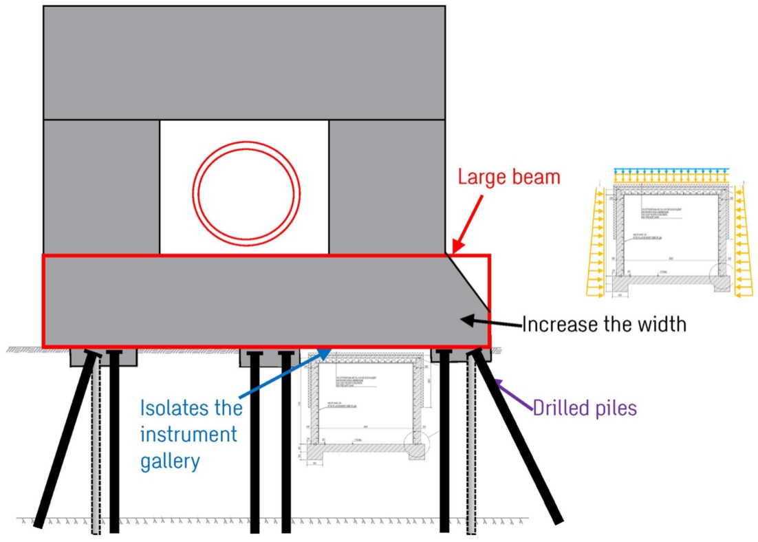
Fig. 27.
Two possible solutions for the interface between beamline and instrument gallery outside the D03 hall. A: only the ceiling of the gallery is lowered. B: both ceiling and floor of the gallery are lowered.
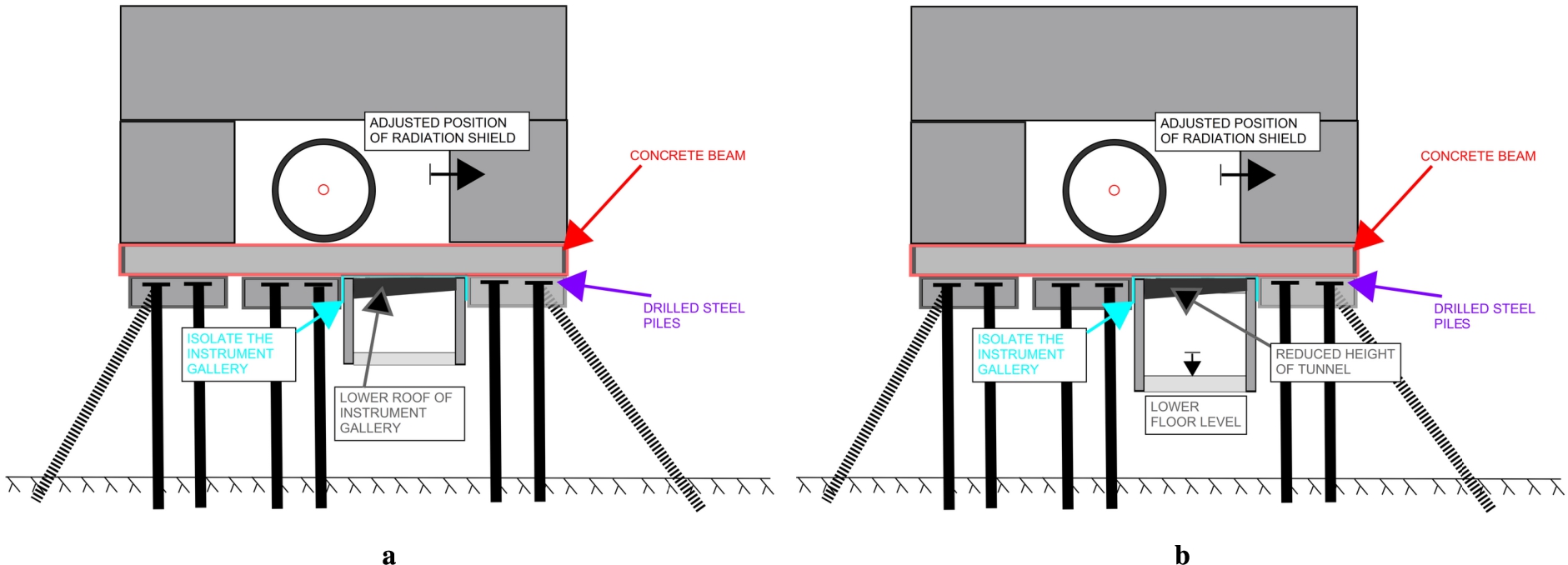
Fig. 28.
Two possible solutions for the interface between beamline and instrument gallery inside the D03 hall. A: only the ceiling of the gallery is lowered. B: both ceiling and floor of the gallery are lowered.
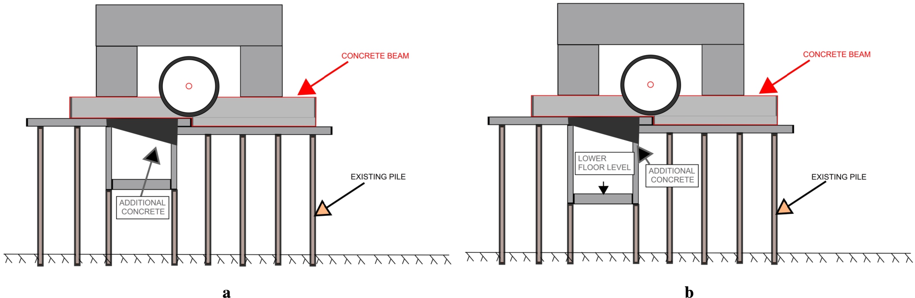
Additionally, the beam serves as shielding for the instrument gallery. Figure 27 shows a more concrete example for how to implement this in the case of position 4 from Fig. 23, situated outside the D03 hall. The same principle is shown in Fig. 28 for inside the experimental hall (position 3 in Fig. 23). In each figure, two possible solutions are presented, both featuring a concrete beam positioned between the gallery and the beamline, supported by drilled steel piles. Lowering the gallery ceiling is necessary to implement these solutions, and additional shielding material is placed inside the instrument gallery in both cases. In the simpler approach, apart from lowering the ceiling (Figs 27a and 28a), the instrument gallery floor remains unchanged. However, it might be necessary to retain the current size of the gallery and to also lower the gallery’s floor. Figures 27b and 28b therefore show a scenario in which the floor of the gallery is also lowered.
10.The NNBAR focusing reflector
The NNBAR reflector system plays a pivotal role in achieving the goal of a performance increase of three orders of magnitude compared to the previous experiment. The primary requirement for the reflector is to efficiently collect the highest fraction of neutrons emanating from the LBP and direct them through the magnetically shielded region toward the annihilation target situated around 200 meters away. Given its size and stringent requirements, this optical system is likely to be one of the most intricate ever developed in the field of neutron research. The design and optimization of this system are detailed in the following section.
10.1.The optimization of the focusing reflector
In the optics simulations in this paper, calculations of the FOM are made using the exact uninterrupted flight time
To facilitate comparison with the previous ILL experiment [43], the FOM is normalized following the procedure described in Reference [15]. The ILL experiment ran for one year. As a result, the FOM is quantified in terms of ILL units per year. A value of
Fig. 29.
The sensitivity
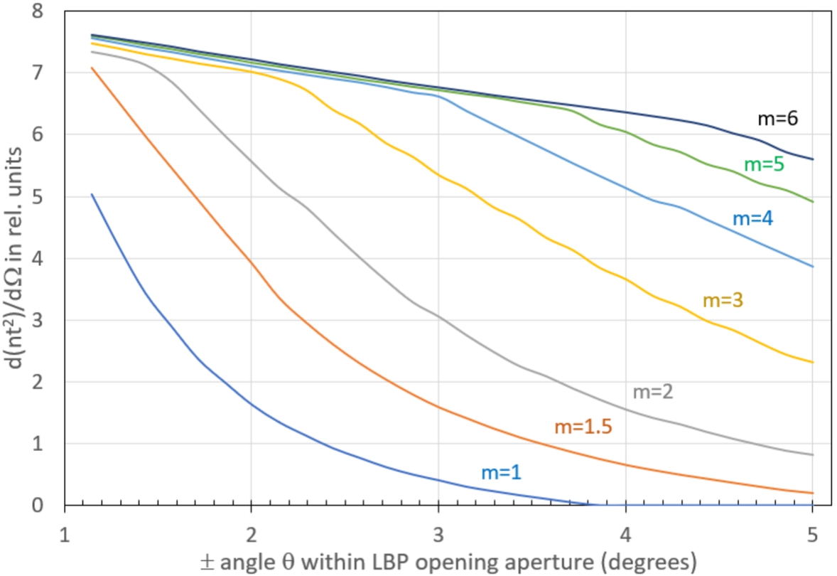
With the above discussion of sensitivity in mind, the concept of the elliptical focusing reflector [123] can be used. Lambertian brightness emission from a cold neutron moderator surface can be intercepted by a large open aperture and super-mirror reflector elements installed within this aperture. This directs neutrons to the annihilation target by a single reflection. An important performance parameter of super-mirror reflectors is the m-value [79]. Given an aperture opening of
Table 4
Gains in FOM that can be achieved by increasing the m-value of a nested mirror reflector that covers an opening of
| m-value | 1 | 1.5 | 2 | 3 | 4 | 5 | 6 | 7 | 8 |
| Relative gain | - | 1.11 | 0.55 | 0.51 | 0.16 | 0.06 | 0.01 | 0.00 | 0.00 |
| Absolute gain | - | 1.11 | 2.29 | 3.97 | 4.74 | 5.09 | 5.17 | 5.23 | 5.23 |
10.2.Nested mirror optics
A possible architecture which transports neutrons diverging from a source to a detector is an elliptical guide. The surfaces of such a device have the shape of an ellipse where the focal points coincide with the centre of the source and the detector, respectively [201,202]. An ellipse has the optical property that a beam that emanates from one of its focal points is reflected directly to the other one. Since this feature does not apply to rays starting not at the focal points, the ellipse is therefore a non-imaging device. Nested layers of several guides are able to build up a spatial tight optical component. If the outer layer of such a nested elliptical guide is given, the inner layers can be designed in a recursive manner such that the layers will not shadow themselves. In the diagram shown in Fig. 30 the construction principle is shown. The finite size of the optical layers is currently not taken into account.
Fig. 30.
Schematic of a nested elliptical guide. M and
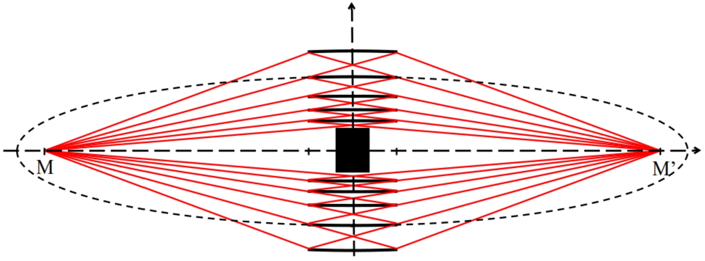
Fig. 31.
Types of nested optical components: a) mono planar b) double planar c) cylindrical.
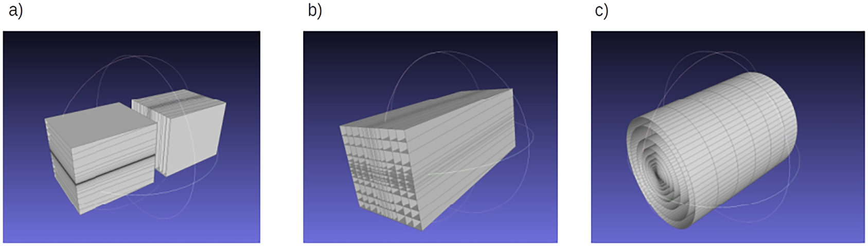
Different nested layouts of the reflector that are symmetrical around the z-axis are possible. These are (a) a mono planar, (b) a double planar, and (c) a cylindrical system. In Fig. 31 three dimensional diagrams of the different types are shown. In a double mono planar reflector, neutrons would have to be reflected twice in order to be directed to the center of the detector. For the cylindrical symmetrical case, only one reflection is needed. The mono planar reflector comprises two separated devices that are rotated by ninety degrees with respect to each other such that one component acts as a horizontal and the other as a vertical reflector. From an engineering perspective this configuration seems to be particularly promising.
A difficulty of the nested reflector design is the thickness of the glass substrate which is used for the construction of the stable high-quality industrial super-mirrors. Recent developments of self-sustaining substrateless super mirrors [174] offer an elegant possible solution to this problem.
10.3.Magnification of an elliptical reflector
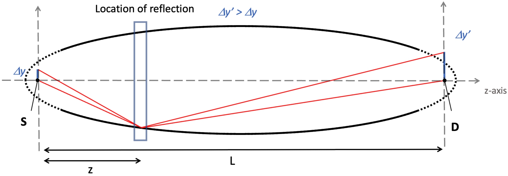
For any portion of a perfect (without accounting for gravity effects) rotational ellipsoid surface, a point-like emission source in one focal point is projected exactly to the image point in the other focal point. However, as is the case for any realistic optical system, if the source point is displaced from the ellipsoid focus laterally to the optical z-axis then the image point will similarly be laterally displaced with a magnification factor. Figure 32) summarises this situation. The magnification M for an off-axis point of height
Fig. 32.
Off-axis magnification of an elliptical reflector. The origin at the source S in the left focal point, L is distance between focal points and to the detector D, and z is the coordinate of reflection along z-axis. Ghe off-axis height at the source is given by
Since the size of the source plays an important role in the capability of the reflector to transport neutrons from it to the detector, the properties and parameters of the focusing reflector are simultaneously optimized with the design of the cold moderator in an iterative process.
Fig. 33.
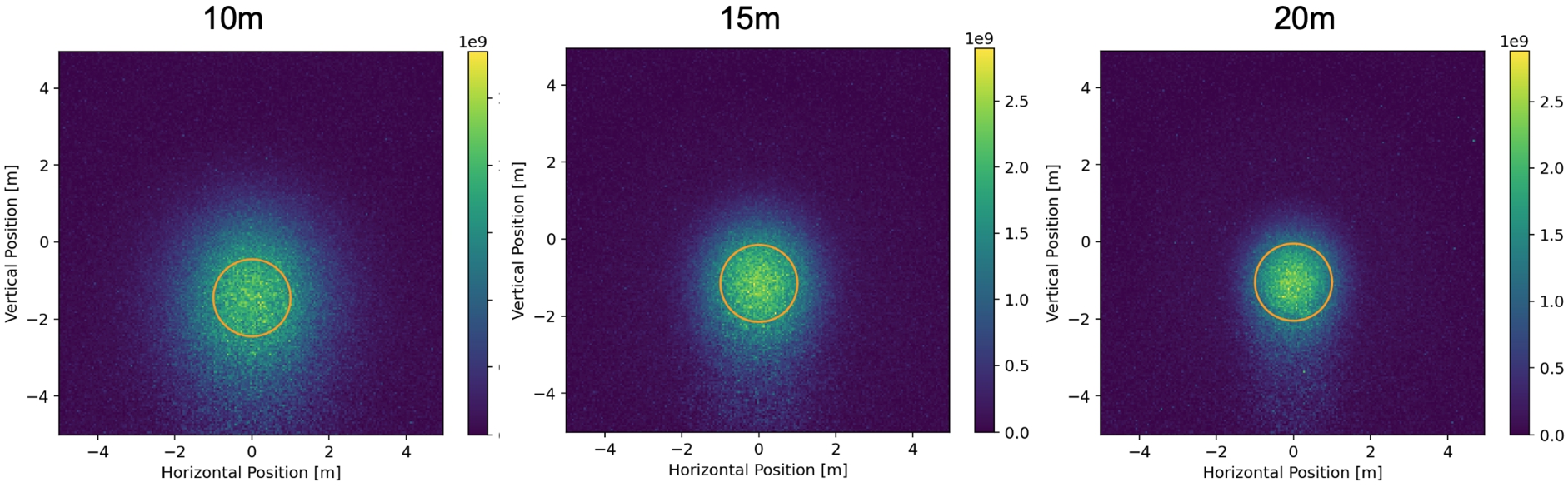
The impact of magnification is illustrated using a 4-level nested elliptical reflector with a length of 10 m, positioned at various starting locations. The representation shows the neutrons arriving at a distance of 200 meters, weighted by the square of their uninterrupted flight time. The orange circle designates the estimated location of the actual antineutron detector, with a radius of 1 meter. The degree of magnification diminishes as the reflector’s starting position is farther from the source. However, it’s important to note that the FOM is greatest for the 15-meter plot. This variation in FOM is essentially a trade-off between achieving effective focusing and covering a broader solid angle.
10.4.Basic reflector setup and simulations
The principal setup for the reflector that is under study has been already shown in Fig. 30. The optic is supposed to start at a minimum distance of 10 m from the moderator center and the detector is placed 200 m away from the center of the moderator. The flight time is measured from the point in time of the last interaction (reflection) with the optic. The transversal dimension of the reflector is bounded by a maximum assumed tube width and height of 3 m. Gravity is turned on for all simulations.
Fig. 34.
Overview of the simulation strategy.
To facilitate comparisons between various geometries and the precise positioning of the reflector system, neutron ray-tracing simulations are conducted using McStas [196]. In McStas, the instrument components are defined using a high-level language, which is subsequently compiled into C-Code to execute the Monte Carlo simulations.
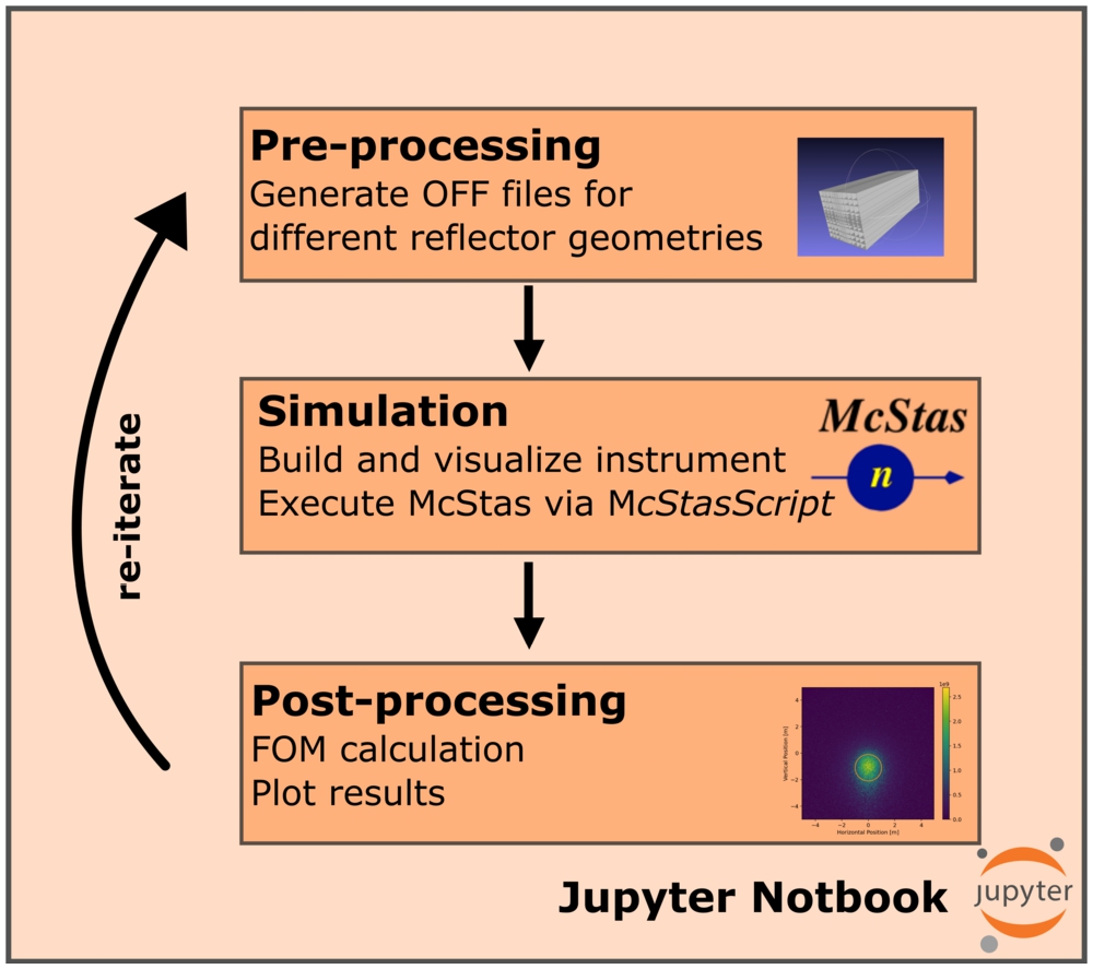
An extension called McStasScript 33 enables the control of McStas using Python scripting (e.g. in JupyterLab 44 a web-based interactive python development environment). This allows for the entire simulation to be managed and executed within a unified environment. Results can be easily accessed for post-processing tasks, including calculations of the FOM and generating plots. The source term is implemented using an
Fig. 35.
Source term calculation with MCPL. The particles are emitted from the moderator window, but already forward propagated to a distance of 2 m, just before the entry of the LBP.
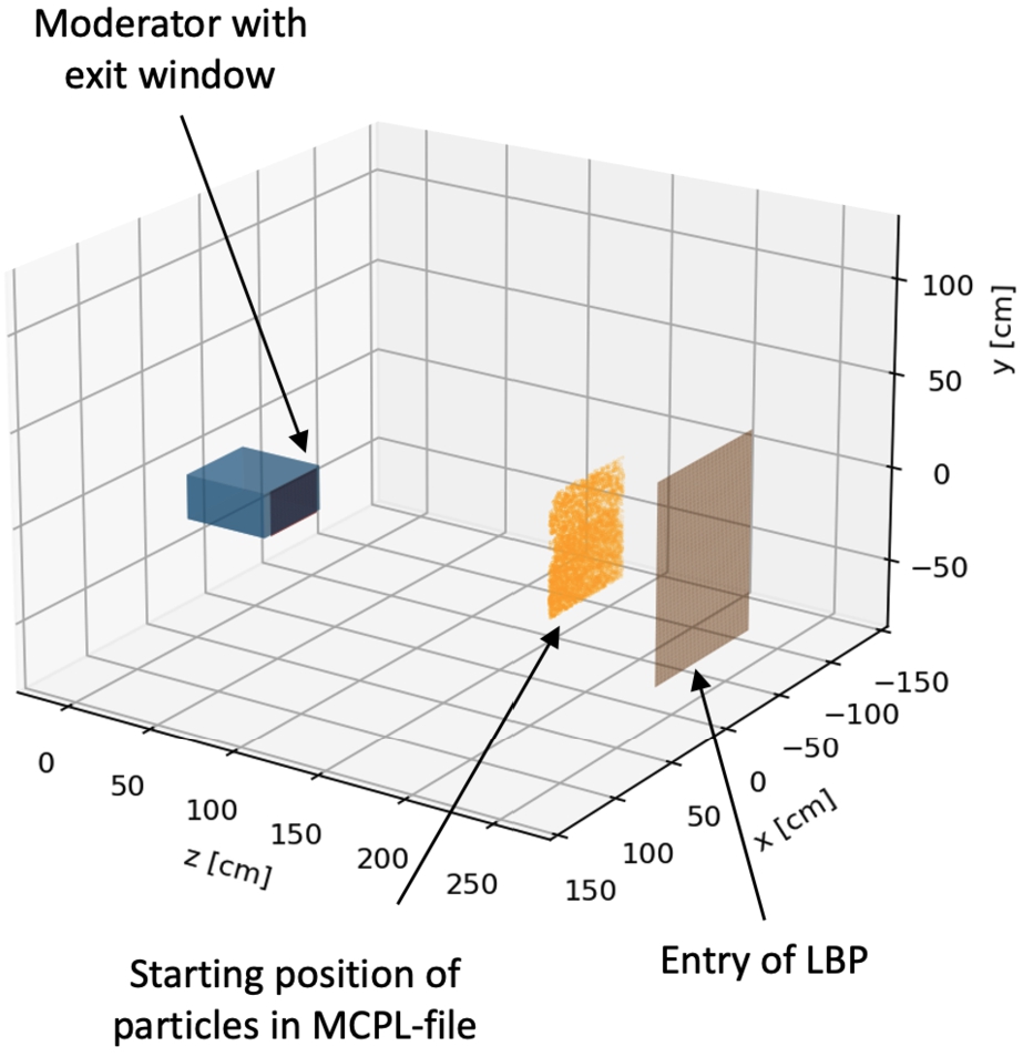
The geometry of the optics is described in the plain text, object file format (OFF-File). This file is automatically generated from a set of input parameters using Python functions. The OFF-file is subsequently employed as input for the McStas component called Guideanyshape. This component is responsible for defining and positioning the reflector. Additionally, the LBP is also represented as an OFF-file and is described using the Guideanyshape component. Neutrons that collide with the walls of the LBP are absorbed. A
By conducting simulations with different designs, utilizing various geometries, and adjusting various reflector parameters (e.g., starting position, length, etc.), a substantial number of optical configurations can be explored to identify optimal parameters. Figure 34 illustrates the general sequence of a typical simulation cycle.
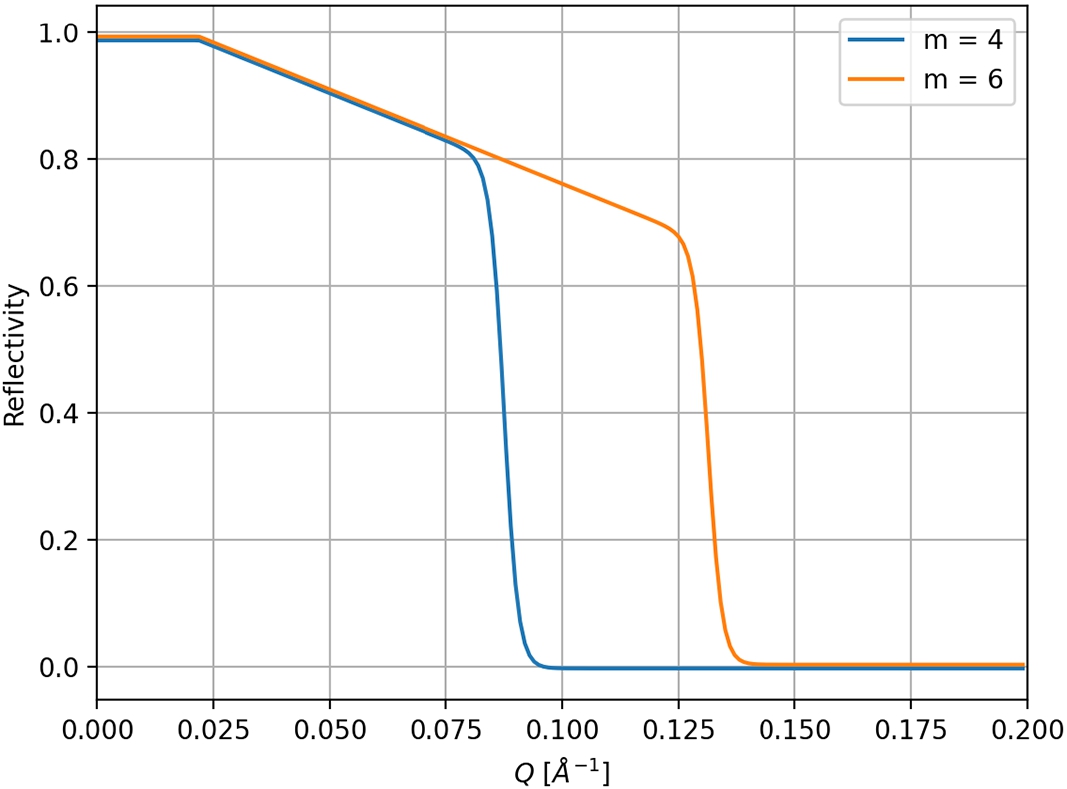
The reflectivity R of the supermirror is calculated in McStas by applying an empirical formula (Equation (10)) derived from experimental data [195].
Here
10.5.Construction of the nested optics
If the outer layer of a nested elliptical guide is given, the inner layers can be constructed in a recursive manner. A sketch of the construction is shown in Fig. 37 (y and z axis have been chosen in to comply with the coordinate system used in McStas). The source S and the detector D are located at the ellipses’ foci.Here,
Fig. 37.
Schematic diagram showing how the inner nested layers are constructed from the outer ones.
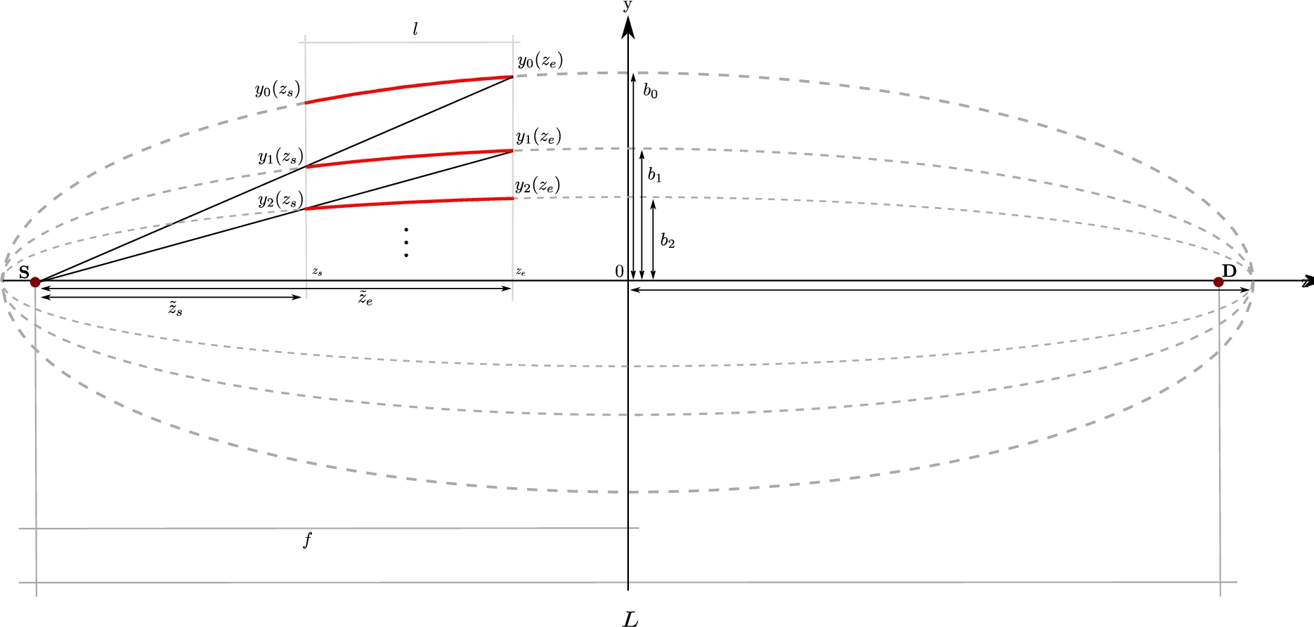
In these expressions,
10.6.Baseline design and the differential reflector
As a starting point for the simulations, a “baseline” design was defined for comparison purposes. This baseline design consists of a cylindrically shaped elliptical reflector with a single layer. The key parameters of this design include: distance of 200 m between the two foci and a small semi axis b of 2 m. The center of the source (moderator) is located in one focus, while the center of the detector is located in the other focal point. The reflector covers the part of the ellipse that starts at 10 m from the source and ends at a distance of 50 m and is therefore 40 m long. For this standard baseline configuration, various aspects of the NNBAR experiment have been studied, including different sizes of the cold source moderator (see Section 2 of Reference [161]), the neutron emission spectra, and the beamline design. This baseline design scheme has, in addition, been previously used for optimization of parameters and for comparison of several NNBAR configurations in previous publications [15,100,148].
A McStas simulation performed with this reflector with the horizontal axis at the center of LBP gave a
Fig. 38.
(Left) 3D visualization of the 40 m long baseline reflector (axis are not in scale). (Right) result of a McStas simulation with the baseline reflector for an accelerator power of 2 MW. The orange circle marks the detector area of 1 m radius. The FOM is 333.
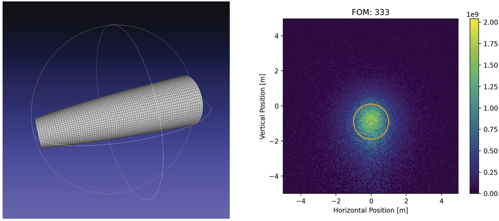
Given that the center of the lower moderator is approximately 20 cm below the axis of the LBP (as illustrated in Fig. 3 of HighNESS Conceptual Design Report Volume I), a symmetrically placed reflector relative to the moderator may not effectively utilize the entire aperture provided by the LBP.
To cope with that issue the concept of a “differential reflector” was proposed [100]. The reflector is positioned exactly in the middle of the LBP but has a distorted ellipsoid shape (See Fig. 39). The constituting panels fulfill the solution of a coupled differential equation, to behave on each position like an elliptical mirror and form a continuous surface. This reflector focuses and bends the neutron beam by a few degrees in the vertical direction at the same time. This will allow the preservation of the FOM with the horizontal beam axis between the centers of the cold source and the annihilation detector.
Fig. 39.
Depiction of the differential reflector.
McStas simulations performed show the comparability of this layout to the baseline design. With the “differential reflector” a
10.7.Optimization of the nested mirror reflector options
Fig. 40.
Result of simulations for a nested double planar reflector of length 10 m (see inlay) for 2 MW (green) and 5 MW (orange) accelerator powers of the ESS. (Left) variation of the starting point of the optic. (Right) effect of increasing the number of nested levels.

The optimal parameters for various nested mirror optics geometries are determined through extensive simulations, and the resulting figures of merit (FOMs) are compared. Two such parameter scans are depicted in Fig. 40 for a double planar nested reflector with a length of 1 m. The scan for the
Regarding the number of nested levels, there appears to be a point of saturation where adding more levels does not lead to a significant further increase in the FOM. This suggests that a balance must be struck between the complexity and cost of the optics system and the achievable sensitivity.
For the simulations of the mono-planar components, the arrangement with mirrors in a horizontal layout was consistently placed in front of the one with mirrors in a vertical layout. This choice was made with magnification in mind. Since the moderator has dimensions of approximately 40 cm in width and 24 cm in height, it is advantageous to have the vertical component with less magnification positioned farther away from the moderator. As the components become shorter, this effect becomes less pronounced.
10.8.Summary of the simulation results
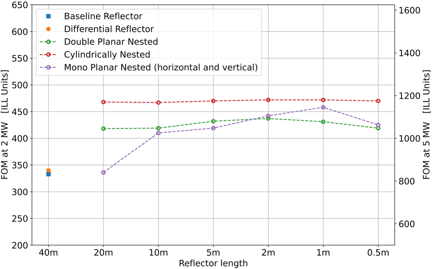
In Fig. 41, the results of the simulations for the various reflector geometries are summarized. The nested components consistently achieve significantly higher FOMs compared to the baseline or the differential reflector. Notably, the cylindrical components slightly outperform the planar ones. This advantage arises because the former (latter) require only one (more than one) reflection to reach the target. In general, the nested components offer gains of at least 20% over the baseline reflector in terms of FOM.
Fig. 41.
Collected FOMs for different reflector geometries for accelerator powers of 2 MV and 5 MW.
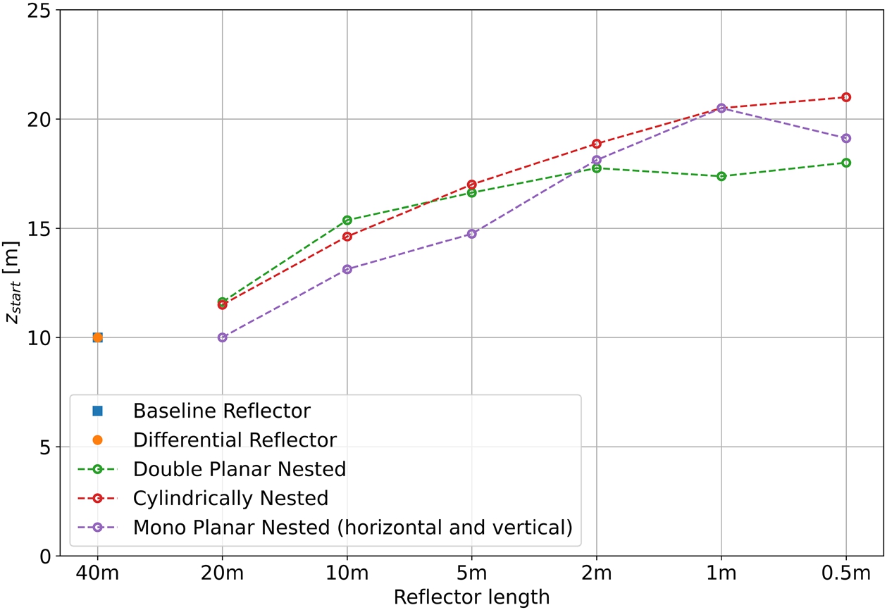
The results regarding the optimal starting locations, denoted as
Fig. 42.
Starting position
10.9.Simulations for a physical model of the experiment
The studies conducted in the previous sections did not consider a detailed beamline layout, apart from the limitations imposed by the LBP. To assess the potential impact of further constraints related to the presence of neighboring instruments (e.g., the LOKI instrument located in close proximity to the NNBAR beamline) and the size of the vacuum tube, additional simulations were performed with the following modifications:
A first rectangular aperture after the LBP at 7.9 m of size 1.8 m × 1.63 m vertically centered at 0.84 m from the top.
A second rectangular aperture after the LBP at 10 m of size 2.2 m × 2 m vertically centered at 1 m from the top.
A circular aperture at 17 m (respectively after the reflector for starting positions that are larger) of radius 1.5 m centered symmetrically.
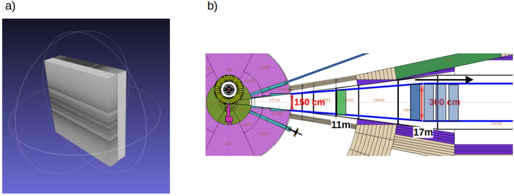
As a reflector for this study, the monoplanar type with a length of 0.5 m has been chosen (as shown in Fig. 43 a) for representation). The reason for this choice is that the construction of this reflector poses fewer engineering challenges compared to the other geometries.
Two possible scenarios for the locations of the reflector that are shown in Fig. 43 have been studied:
Inside the bunker at 11 m.
Outside the bunker starting from 15 m.
Fig. 43.
Left side: depiction of the reflector used for the simulations. Two mono-planar (MP) nested mirror assemblies, each of 0.5 m length. Right side: sketch of the placement of the reflectors in the physical model of the experiment; inside bunker position at 11 m (green); outside bunker (starting at 15 m) (blue).
For both scenarios, the length of the experiment was also varied to study the impact of longer NNBAR baselines on the FOM. The results in the following sections are presented for a 2 MW accelerator power, but they can be easily scaled to a 5 MW power scenario.
10.9.1.Results for reflector located at 11 m from the source
The results of the simulations for a longer baseline reflector at a distance of 11 m are shown in Fig. 44. For a detector at 200 m away from the moderator, a FOM of 221 is achieved. Increasing the experiment’s baseline length further only leads to marginal gains. This is primarily due to the high magnification factor at this position, which becomes even more significant as the baseline is increased. As a result, the image at the detector becomes smeared out, as depicted for several lengths in Fig. 44.
Fig. 44.
Results of simulations for a reflector placed at 11 m. The plot on the right shows the shift of the center of intensity on the detector due to gravity for longer baselines. At the bottom, images for selected lengths of the experiment are shown. The blurring is due to the increasing magnification.
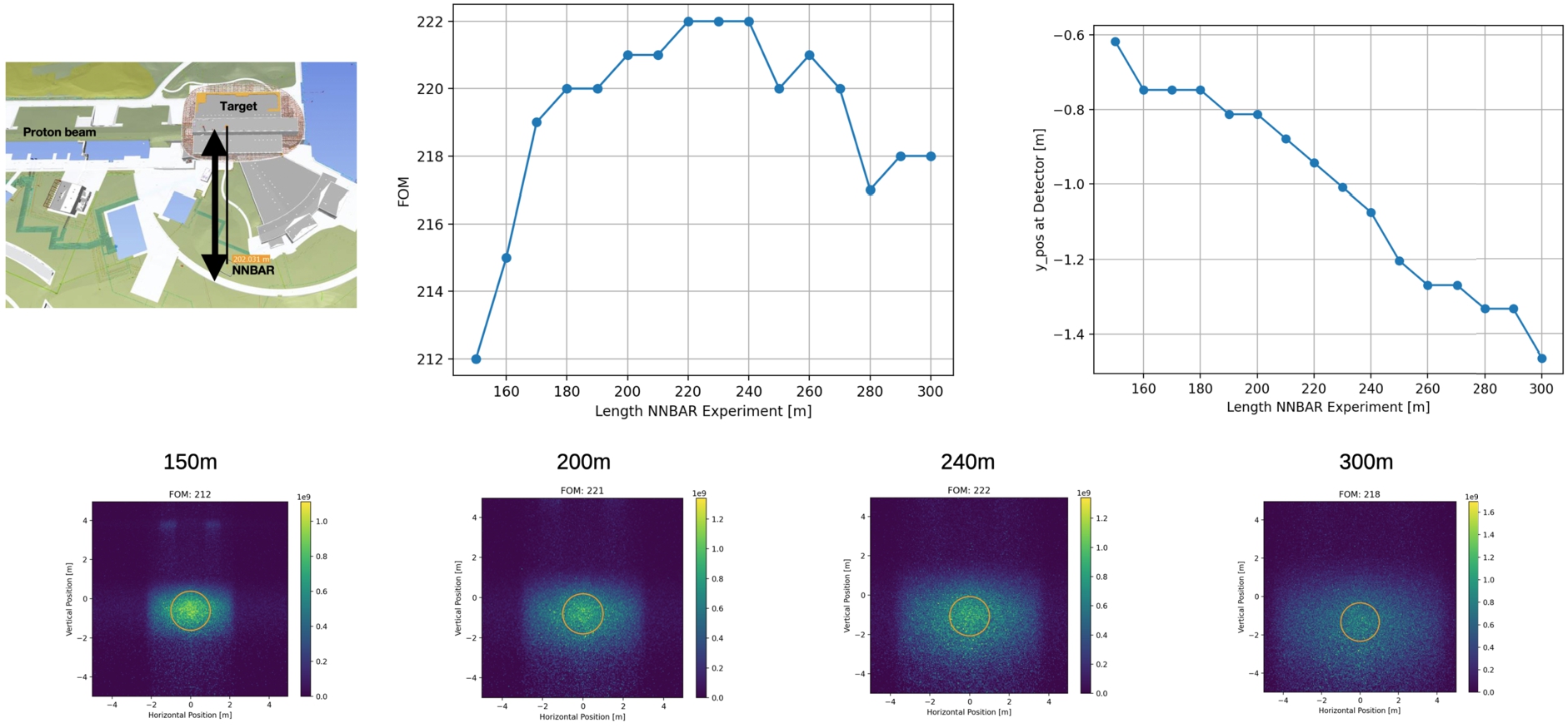
Fig. 45.
Results of simulations for a reflector placed beyond 15 m as a function of the length of the experiment.
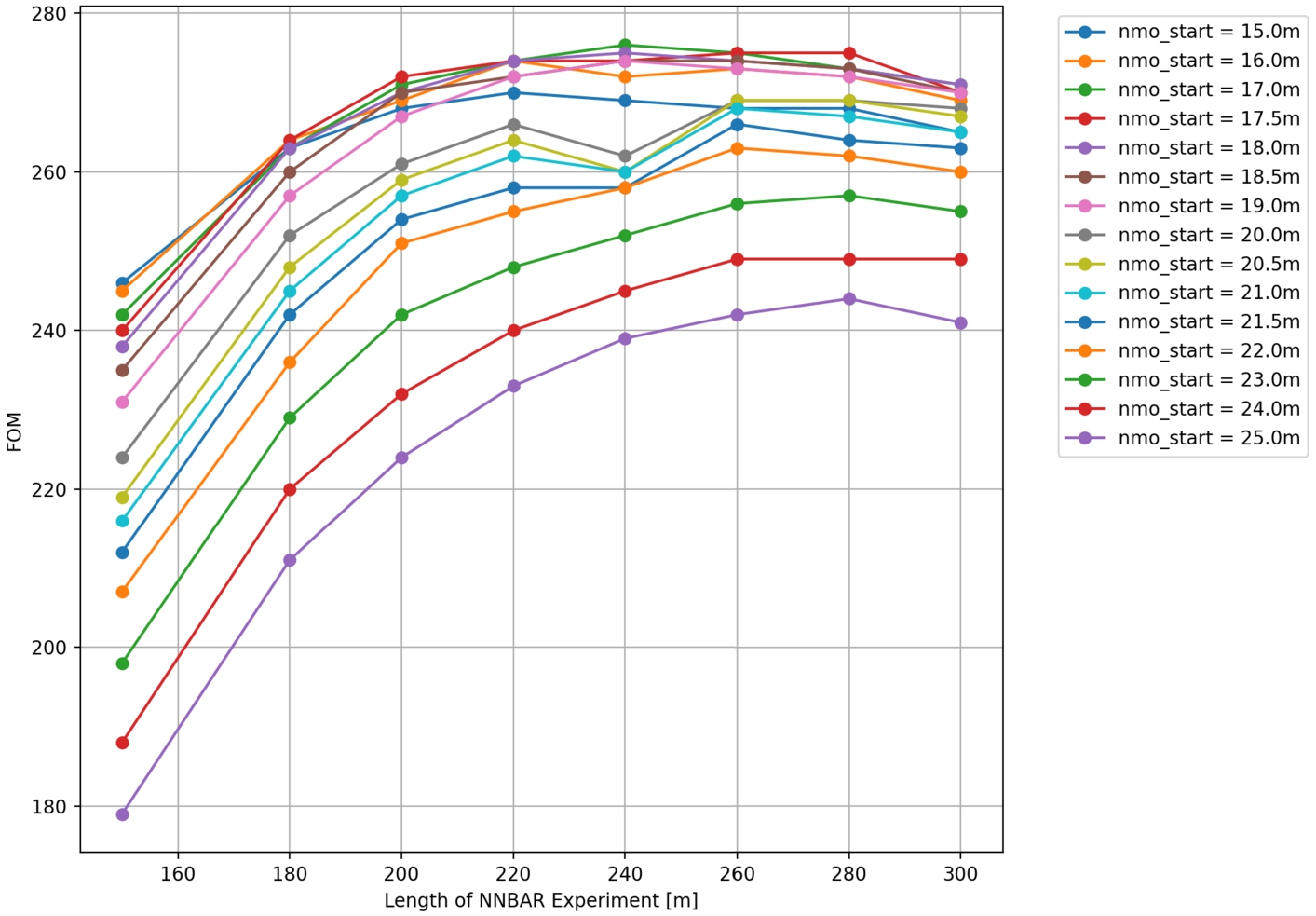
10.9.2.Results for a reflector located beyond 15 m
In this scenario, both the baseline of the NNBAR experiment and the starting position of the reflector have been varied. The results are visualized in Fig. 45 and Fig. 46.
Figure 45 shows that the FOM remains relatively constant at lengths of about 200 m. The optimum starting location for the optics outside the bunker scenario is found to be at about 18 m, with a FOM ranging between 270 and 275.
These results suggest that, within the considered parameter space, a baseline beamline length of approximately 200 m and a starting location of around 18 m outside the bunker could provide an optimal configuration for the NNBAR experiment.
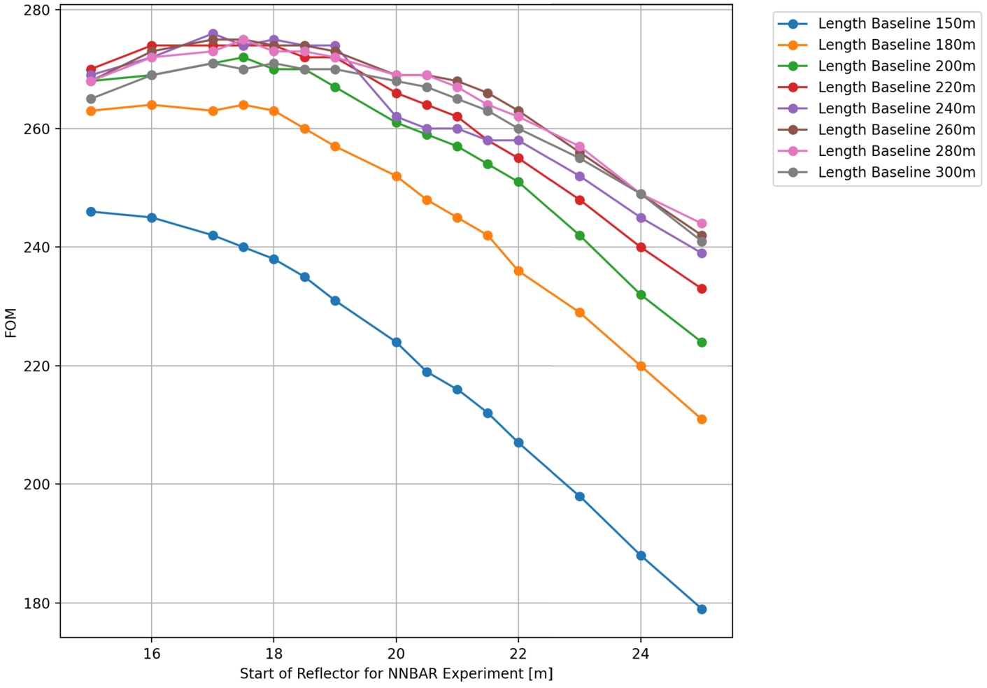
Fig. 46.
Results of simulations for a reflector placed beyond 15 m as a function of the starting position. Alternative visualization of the same data as in Fig. 45.
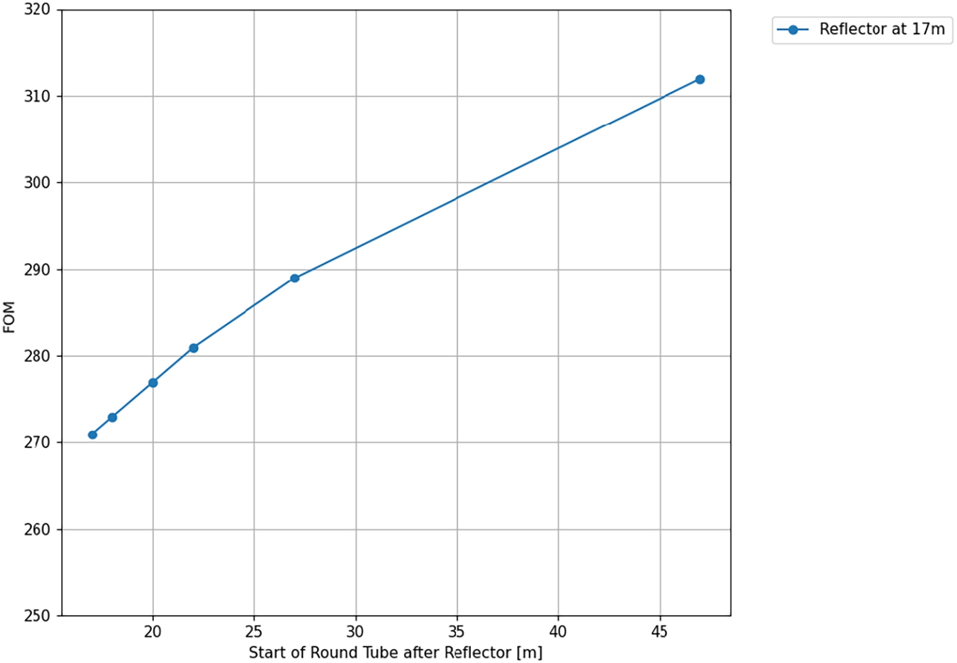
The results indicate that using a square-shaped tube section after the optic, which transitions to a circular cross-section after a certain distance, can improve the performance of the NNBAR experiment. Figure 47 shows the results for a reflector placed at 17 m with different lengths of the square-shaped section.
For instance, a length of 20 m for the square-shaped section would result in a FOM of 300. This suggests that modifying the beamline geometry in this manner can lead to a substantial improvement in experimental sensitivity. This configuration used for estimations of the full sensitivity of the NNBAR experiment that are given in Section 17.
Fig. 47.
Results of simulations when adding a squared shaped tube section after a reflector placed at 17 m. The FOM increases with the length of the section.
11.Magnetic shielding
Magnetic fields must be sufficiently small so as not to inhibit the transition between a neutron and an antineutron owing to a lack of degeneracy between the particles caused by their opposite magnetic moments. It is necessary to achieve the quasi-free condition such that the probability of a transition becomes proportional to the square of the propagation time. Maintaining a magnetic field of less than approximately 5–10 nT satisfies this condition [84,148].
Neutrons travelling 200 m inside a shielded environment will nevertheless by subject to a time-varying field in the rest frame of the particle. This results in gradients and spatial and temporal distortions in the field. It was shown in Reference [84] that such effects do not significantly suppress the neutron–antineutron transition. The most important quantity is the magnitude of the average field. The goal for NNBAR is therefore to permit neutron propagation with an average field experienced along each neutron trajectory of less than around 5–10 nT. An additional constraint is that, in order to avoid interactions, the neutrons move in a vacuum. A shielding system, described below, has been designed [39], which gives a typical field of around 5 nT.
11.1.Magnetic shielding concept
The shield concept is illustrated in Fig. 48 and is simulated with COMSOL [81,82]. The model comprises a two-layer octagonal mumetal shield combined with a stainless steel vacuum chamber, which also aids with the shielding. In addition, an external excitation coil is arranged around the shield to monitor the performance.
Mumetal shielding gives a static lowering of the magnetic field in addition to damping changes in the external magnetic field of up to about 10 Hz. The shielding of higher frequencies is given by the combination of the conductivity of the vacuum chamber and the mumetal.
Fig. 48.
Left: the 200 m long and 2 m inside diameter arrangement. This consists of a pair of octagons made from mumetal, with a 200 m length and a stainless-steel vacuum chamber separating them. Right: a shield cross section. A logarithmic scale magnetic field magnitude is shown. (1) outer mumetal shield; (2) vacuum chamber; (3) inner mumetal shield.
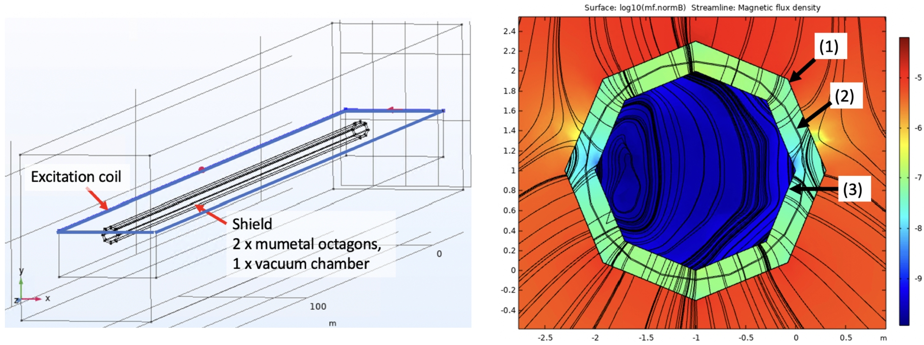
The design of the mumetal shield is based on a proven small-scale design of the magnetic shield which is used for an atomic fountain [197]. This comprises mumetal sheets, deployed in an octagonal shape and which are clamped together. Overlaps of 50 mm width of the mumetal sheets are foreseen to ensure proper magnetic flux connection while being a reasonable compromise with magnetic equilibration. Using this approach, the independent assembly and detachment of the shield parts can be done when needed. The vacuum chamber can be arranged in between the mumetal layers or inside the inner mumetal layer.
For a low magnetic field, magnetic equilibration of the mumetal is required [27] through a set of coils. These surround each shield layer independently as a toroidal coil. The shield diameter is determined by the volume accessible to the neutrons together with a distance of around 20 cm to the shield walls, where the fields after equilibration are too high for the experiment. Furthermore, the gap between the mumetal shells is estimated from simulations and set to a minimum of 20 cm.
11.2.Simulations
Figure 48 shows a schematic diagram of the shield modelled in the simulation. For the optimization of parameters, the shield was deployed inside a static background field which is normal to the shield axis. The influence of various static fields from other ESS instrument magnets at LoKi, ESTIA, SKADI, DREAM, HEIMDAL and T-REX [94] were also considered. Representative tests of steel rebar from magnetic concrete and structures were additionally made. A large external coil is deployed surrounding the shield. This produces a magnetic field mostly perpendicular to the shield axis. The coil is placed closer to one open end of the shield than on the other side in order to also study the effect of fields entering the shield longitudinally. Estimates of shielding efficiency were then made for 1, 10 and 100 Hz frequency, which included permeability and currents. The estimation of DC field reduction is not quantitatively possible for fields of very low magnitudes via a magnetostatic approach. However, it should be pointed out that the effect of magnetic equilibration is both well studied and tested and, in specific and simple scenarios, can be calculated [182,183]. It can thus be scaled from a magnetostatic simulation based on a typical mumetal anhysteric curve. Figure 49 shows the fields inside the shield arising from excitations of frequencies in the range of 1 to 100 Hz, together with an external excitation which has an identical amplitude.
Fig. 49.
Field inside the shield (cross section in middle region), for 1, 10 and 100 Hz external excitation.
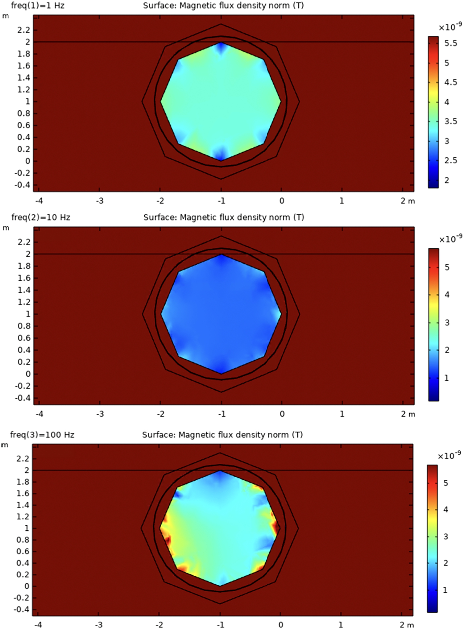
From the ratio of outside and inside magnitude, the shielding factor
Although the equilibration efficiency is not simulated quantitatively but scaled from experimental findings, the field distribution inside the shield after equilibration is modeled, as seen in Fig. 50.
Fig. 50.
The expected field pattern from the magnetic equilibration process.
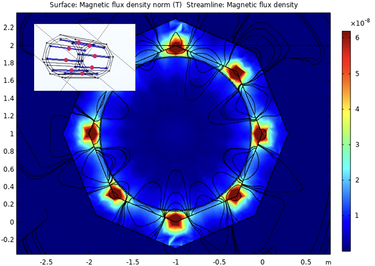
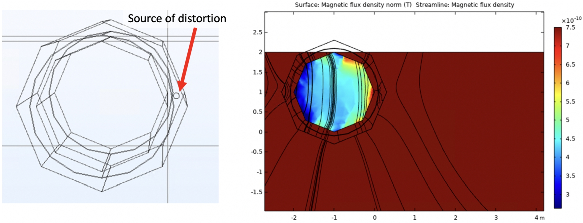
Magnetic equilibration can be realized, as studied in the simulation, using 8 turns for each octagon, with 80 Amp-turns. An additional point to consider is the effect of local magnetic distortions which can have as their origin, e.g. the vacuum chamber or an outside source. The modelling of these is shown in Fig. 51. A typical scenario could be a magnetic weld in the vacuum chamber, which can be >1000 nT extending over distance of few centimeters.
Fig. 51.
An example of a magnetic distortion arising to due to a magnetic weld. The impact on the inside field after equilibration is shown.
A Monte Carlo study which tracked particles inside the shield using simulated residual field maps has been carried out. This showed that the efficiency loss due to the presence of the small but finite magnetic field is around several per cent.
12.NNBAR vacuum
As previously explained, it is necessary to transport neutrons within a magnetically shielded and low-vacuum environment. For quasi-free neutrons, the vacuum pressure should be maintained below
The ESS monolith was designed to be able to operate with He atmosphere (100 kPa) or at a low pressure
The vacuum vessel will house the neutron optics (Section 10.1) in a vacuum environment and will provide support for the external magnetic shield (Section 11) along the entire length of the beamline. During the optimization of the NNBAR optics design, the following approach was adopted for the vacuum pipe. Initially, a rectangular vacuum pipe is used from the LBP up to the location of the optics, which lies around 17 meters after the moderator as discussed in Section 10.9. Following this, the design transitions to a cylindrical vacuum pipe with a 3 m diameter, extending up to the detector area, where it will then reduce to a 2 m diameter.
A combination of mechanical pumps (dry rough and turbo-molecular) units for pump down and a combo-type (sputter ion pump and non-evaporable getter) are currently planned as a permanent pump solution to minimise vibration on the optics system and to assure a low level of physical access during the periods of operation.
13.The NNBAR detector
The ultimate goal of the NNBAR detector is the reconstruction of an annihilation event and rejection of background. The signature is an isotropically produced multi-pion final state (between 2 to 8, with an average of ∼5) with a centre-of-mass energy of up to around 1.9 GeV. The constraints in designing such a detector are as follows.
All primary particles hitting the detector should be identified and the directions and energies of annihilation and nuclear products must be measured. Given the constraint of the field-free propagation region, no magnetic field is used in the tracking system. Due to the rare nature of the process being measured, a statistical correction cannot be used, i.e. the determination of an inferred signal contribution from a large number of selected events comprising signal and background processes. As a consequence, combinatorial mistakes must be suppressed. Since the annihilation occurs in a nucleus and not in free space, the rejection power of some observables such as invariant mass and total energy will be degraded, as discussed in Section 14.3. This implies that some of the overall demands on the calorimeter energy reconstruction for the signal final-state particles can be relaxed. It is also important that all particles from background processes are identified as such and that these should not degrade the signal, e.g. due to background events piling up in-time with a signal event. Finally, it is important that technological and geometrical choices are made such that the final detector is affordable. These points represent an ideal case. However, in practice, compromises between the different choices will be needed. In order to identify an annihilation event, a combination of different types of evidence from the detector are needed.
The first type of evidence to guide the detector design is topological. A common vertex of origin in the carbon foil from several charged particles is helpful.55 If a neutral pion is identified, it can be associated with the same vertex as the charged pions. This requires tracking in three dimensions. Three dimensional tracking will allow excellent space resolution of all recorded events.
Figure 52 shows the charged-pion multiplicity from antiproton annihilation in 12C. Antineutron annihilation in 12C would give states in the same proportions as for antiproton annihilation. A simulation is also shown of antineutron-nucleon annihilation in carbon, which is used in this work and which agrees well with the data. Predictions are also shown for antineutron-nucleon annihilation in argon, which show minimal differences with expectations for 12C. In 10% of the cases there is only one outgoing charged pion, whereas in 88% of the cases there are two or more charged outgoing pions. The charged pions are the cornerstones of the annihilation topology, since these can be tracked and be used to reconstruct the event. Beyond the charged pions, charged nuclear fragments can also be produced and tracked. For the events that have only one charged pion, a
Fig. 52.
The probability (%) of the formation of a specific multiplicity of charged pions in antinucleon-nuclei annihilation. The solid histogram shows data from
![The probability (%) of the formation of a specific multiplicity of charged pions in antinucleon-nuclei annihilation. The solid histogram shows data from p¯12C interactions. Experimental data: circles-[[19]], squares-[[153]]. The dotted histogram shows a n¯12C simulation ; the dashed histogram shows an n¯Ar simulation. Taken from reference [106].](https://content.iospress.com:443/media/jnr/2023/25-3-4/jnr-25-3-4-jnr230951/jnr-25-jnr230951-g053.jpg)
Another set of evidence comes from conservation of energy and momentum, which is intrinsically connected to particle identification (PID). Since a significant fraction of the available energy (∼30%) corresponds to the rest masses of the pions, accurate PID and thus measurements of the multiplicities of different types of particles are themselves indirect energy measurements. For a final-state with four pions, nearly 600 MeV of the total energy is accounted for in this way. In principle, the momentum and energies of all annihilation and nuclear products should be measured in order to reconstruct event kinematics and exploit event-level characteristics of the signal event, such as the expected isotropy of produced particles.
13.1.Detector choices
A number of technologies were considered. Out of the gaseous trackers, a TPC was chosen. A TPC is ideal for the purpose of pattern recognition in three dimensions with minimal combinatorial ambiguities and has a number of other desirable properties such as providing high precision specific energy loss,
For calorimetry, a scintillator-based hadronic range detector (HRD) and a lead glass electromagnetic calorimeter (LEC) are the chosen technologies for photon and pion energy measurements. A sampling calorimeter was considered [39] for electromagnetic energy reconstruction. But it was found to have lower
The lower energy charged hadrons (p and π) can be stopped gently, by ionization energy loss. The measured energy deposit will then be a correct measurement of the kinetic energy. The higher energies require a substantial amount of material to stop the particle by ionization energy loss. The probability is then high that nuclear reactions will occur before the charged hadron has fully depleted its kinetic energy. An energy deposit will then be a very crude measurement of the kinetic energy. There is no detection way around this fact unless a magnet is introduced. For charged hadrons the energy resolution is poor at high energies and here it will be even worse for hadron calorimetry [198]. Neutral pions decay in almost all cases to 2 photons. A
Figure 53 shows a cut-away of the detector, encased with concrete. This was produced as part of the mechanical construction study (Section 16).
Fig. 53.
Cut-away of the NNBAR annihilation detector.
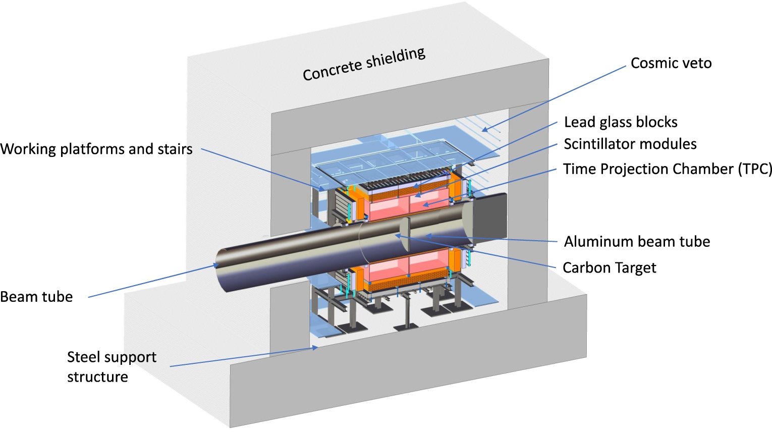
13.2.Detector simulation
A GEANT4 model was developed to describe this detector. The model includes all major material sources (beam pipe, TPC, scintillator staves) though omits smaller items such as electronics.66 The model was used to study light production in the lead glass and scintillator staves.
A microscopic simulation of tracking in the TPC is a formidable and CPU-expensive task. This is not done here. At this point it is most reliable to utilise experiences from TPC’s in operation, mainly the ALICE TPC and its upgrade [10,17,157] which is the most modern large scale installation with decades of prior R&D by many experts. In particular the most performance-driving parameter, the drift length, ∼2.5 meter at NNBAR, is the same as for the ALICE TPC. The NNBAR TPC with its shorter track length may have to carefully optimize the drift conditions near the inner and outer edge of the drift field. The ALICE TPC has operated at low magnetic field which also makes it similar to our zero field. The ALICE TPC with 2.5 m drift length in the drift dimension and with no magnetic field has track residuals (normally claimed as the single point resolution) of about 0.5 mm for tracks parallel to the readout plane. This is moderately better at short drift and worse at long. With a tilt angle, the residuals deteriorate to mm scale. The single point resolution is, however, not the parameter of interest in a TPC where many points per track are measured. It is the track location and direction obtained by a straight line fit to many coordinates which matters. However, the inherent resolution of the TPC is not a limiting factor for the pointing towards the vertex. It is, instead, the fact that the measured track direction outside the vacuum chamber is not the same as inside due to multiple scattering in the chamber tube wall (see Section 14.2).
13.3.Beam tube and target
Neutrons arriving at the experimental hall enter an evacuated aluminum beam tube with 1 m nominal inner radius and 2 cm wall thickness, and encounter a thin (
13.4.TPC
Outside the beam tube is the TPC system, which provides three-dimensional charged particle tracking for event vertex identification and track matching, as well as particle identification capabilities through measurements of the specific energy loss
The TPC is nominally constructed from eight rectangular chambers each 70 cm deep, 200 cm long and 280 cm wide and contains an assumed 80:20 Ar/CO2 mixture.
The TPC chamber walls are constructed from fiberglass. Charges are collected at the anode wall by gaseous electron multiplier (GEM) foils read out by 32-channel mixed-signal SAMPA ASICS originally developed for the ALICE TPC and muon chamber upgrades at the LHC. The SAMPA chips provide a full-on detector readout chain that includes amplification/shaping, digitization, a DSP layer, and readout over multiple parallel 4.8 Gb/s serial links.
The full TPC system contains 256000 GEM channels that can be continuously read out with sample rates as high as 10 MHz, corresponding to more than 5300 4.8 Gb/s serial links.
13.5.HRD
The HRD is a multi-layer calorimeter with plastic scintillator staves that function both as an active material and absorber. It is designed to identify and measure minimum-ionizing energy deposits from low-energy charged pions traversing the scintillator, and is capable of distinguishing between proton and pion tracks by their specific energy loss
The HRD has a nominal thickness of 30 cm deep, and is built from 10 layers of long scintillating staves, each with a thickness of 3 cm.
The full HRD stack corresponds to around 0.6 interaction lengths and around 0.5 radiation lengths. The staves in each HRD layer run perpendicular to those in neighboring layers, producing crossing points for reconstructing minimum ionizing tracks of particles passing through multiple layers. Two embedded wavelength shifting (WLS) fibers running along the length of each stave collect and transport scintillating light to silicon photomultipliers (SiPMs) at the ends and the staves are coated with white reflective paint for optimal light collection in the WLS fibers.
The expected timing resolution of the SiPM stave readout is around ∼1 ns [42], and the majority of staves have SiPMs at both ends, allowing position and timing of hits to be estimated from the light propagation timing differences. An exception is at the “end cap” regions where the stave geometry around the beam tube makes this difficult; in the baseline design these shorter staves are therefore read out at only the stave ends furthest from the beam.
Fig. 54.
Assembly of two SiPM diode arrays and analog front-end electronics at the end of a scintillator stave (left), end-view of a stave with two wavelength shifting fibers installed. This picture is of a prototype stave (reference [92]). The HRD staves in the design presented here are of different dimensions (see Table 5).
![Assembly of two SiPM diode arrays and analog front-end electronics at the end of a scintillator stave (left), end-view of a stave with two wavelength shifting fibers installed. This picture is of a prototype stave (reference [92]). The HRD staves in the design presented here are of different dimensions (see Table 5).](https://content.iospress.com:443/media/jnr/2023/25-3-4/jnr-25-3-4-jnr230951/jnr-25-jnr230951-g055.jpg)
An illustration of SiPM and front-end electronics board (FEB) assembly at the end of each HRD stave is shown in Fig. 54, alongside a photograph of a prototype stave. The WLS fiber ends are aligned by a plastic guide glued to the end of the stave, where they are then cut and polished. A milled aluminum enclosure holding the two SiPMs is mounted over the fiber guide. The enclosure also hosts a front-end electronics board (FEB) with analog amplification, shaping and readout circuitry for the SiPMs, calibration LEDs, and low- and high-voltage power distribution.
This HRD design includes more than 3000 scintillating staves with a combined length of more than 9 km. The staves are read out by approximately 4500 front-end boards and 9000 SiPMs.
The above gives the broad principle of the HRD baseline design. A more segmented HRD with shorter staves of length 40 cm aimed at mitigating light attenuation in the WLS fiber readout and pile-up is possible. This is used here in simulations of signal and background discrimination. The final design depends on details of accurate and reliable estimates of pile-up.
13.5.1.Simulations of staves
GEANT4 simulations have been used to study the expected energy loss for various thicknesses of scintillators.
Figure 55 shows predictions of the range in the scintillator plastic of particles with different values of kinetic energies at the target foil. A scintillator thickness of 2 cm will induce energy deposits of close to 8 MeV for charged pions, and around 18 MeV for protons. Figure 55 shows simulations of energy deposits in 2 cm of plastic by photons produced following neutron capture in the carbon target along with energy deposits from
Fig. 55.
Simulations of particle interactions in the HRD: (a) the range of particle in the scintillator plastic after passing through the vacuum tube and other detector material (b) energy lost in 2 cm of scintillator plastic for a range of particles and energies. Figure from reference [92].
![Simulations of particle interactions in the HRD: (a) the range of particle in the scintillator plastic after passing through the vacuum tube and other detector material (b) energy lost in 2 cm of scintillator plastic for a range of particles and energies. Figure from reference [92].](https://content.iospress.com:443/media/jnr/2023/25-3-4/jnr-25-3-4-jnr230951/jnr-25-jnr230951-g056.jpg)
The generation of photons in a single scintillator bar and their transport through the scintillator material and the wave-length shifting fibers was investigated with a view of taking a parametrization of the measured scintillation photons at the SiPM to provide an estimate of detector response. The number of optical photons reaching the SiPMs at the end of each fiber was determined for different particle types and energies while varying the hit position. Fibres were simulated corresponding to the absorption and emission spectra of Kuraray Y-11 fibres. The refractive index of
Fig. 56.
Left: the number of optical photons reaching the SiPMs as a function of the produced scintillation photons. Right: the ratio of the number of optical photons at the SiPMs over all scintillation photons. The top distributions show muons at a range of energies. The bottom distributions show distributions for a range of particles at 200 MeV kinetic energy.
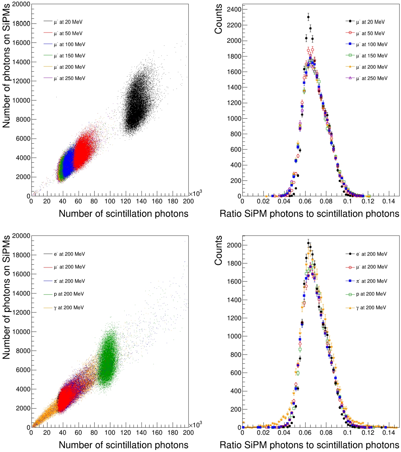
Figure 56 shows the number of optical photons reaching the SiPMs as a function of the number of scintillation photons produced for a stave of size
Fig. 57.
Left: fraction of scintillation photons absorbed by a WLS fiber as a function of distance from the fiber. Right: fraction of WLS photons reaching the SiPM as a function of z.
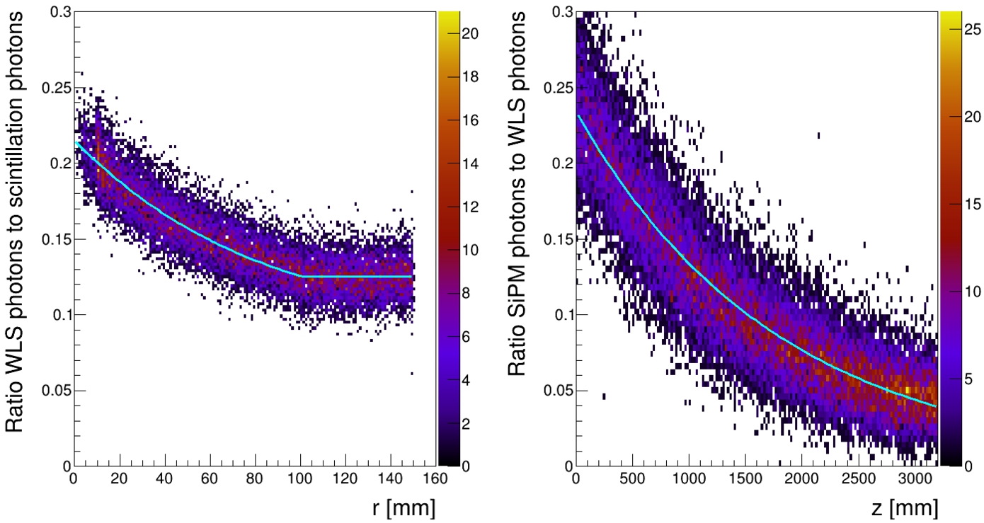
To arrive at a parametrization for the expected number of optical photons at a SiPM, the fraction of SiPM hits is considered to be the product of the fraction of scintillation photons being absorbed in a WLS fiber and the fraction of photons re-emitted by the WLS material reaching the end of the fiber without escaping or getting absorbed as described by Equation (14).
Fig. 58.
Exploded view of an LEC lead glass counter.
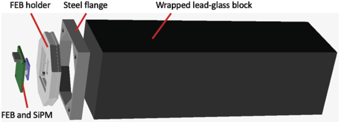
13.6.LEC
Surrounding the HRD is a lead glass electromagnetic calorimeter built from around 32000 instrumented glass blocks. The LEC is designed to measure gammas from neutral pion decays, as well as higher-energy charged pions that are not stopped in the HRD.
An exploded view of an LEC glass counter is shown in Fig. 58. The lead glass block faces have
Since minimum Cherenkov velocity in a material is inversely proportional to its refractive index, a dense flint glass was chosen with high refractive index of 1.67 (Schott SF5 / CDGM ZF2) in order to improve sensitivity to lower energy charged pions. The sides of the lead glass blocks are wrapped with enhanced specular reflective film for improved Cherenkov light collection efficiency. To suppress signals from cosmic particles entering from outside the detector, light-absorbing material at the inward-pointing face is used to minimize reflection of Cherenkov light emitted in the “wrong direction”.
The LEC counters are mounted in the detector using steel mounting flanges glued to the back face of the glass blocks. The flanges are manufactured from martensitic stainless steel with a thermal expansion coefficient similar to that of the glass to minimize stresses at the steel-glass interface. The center of the flange provides wide open areas for mounting the SiPM arrays and LEC front-end boards. The LEC includes more than 32000 SiPM readout channels, corresponding to one SiPM array and front-end board per glass block.
13.6.1.LEC simulations
Simulations with GEANT4 were carried out to estimate the required depth and granularity of the lead glass blocks. The energy resolution for
Fig. 59.
Particle shower containment as a function of lead glass depth for
![Particle shower containment as a function of lead glass depth for 4×4 cm2 lead glass blocks. Figure from reference [92].](https://content.iospress.com:443/media/jnr/2023/25-3-4/jnr-25-3-4-jnr230951/jnr-25-jnr230951-g060.jpg)
Fig. 60.
The number of Cherenkov photons at the back of the lead glass module (detected) and the number of Cherenkov photons generated in the lead glass block versus the deposited energy.
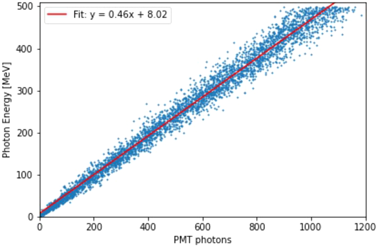
13.7.Cosmic veto
Fig. 61.
GEANT4 model of the cosmic veto detector, including a simplified model of the annihilation detector. The passive shielding has been omitted in the drawing.
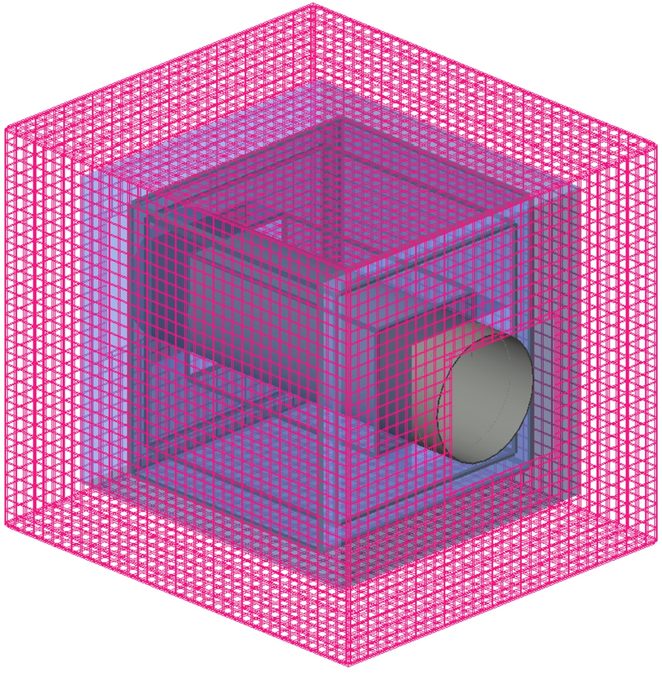
In the previous search for baryon number violation at ILL, cosmic rays were the dominant contribution to the background [43]. A reliable cosmic ray veto system is therefore crucial for the NNBAR experiment. For initial studies, a baseline geometry for the veto detector has been created.
A baseline model for the veto system produced with GEANT4 is shown in Fig. 61. The veto detector geometry is relatively simple, a box with dimensions 6.4 m × 6.4 m × 7.2 m, large enough to contain the NNBAR annihilation detector. It comprises two layers of scintillating staves 20 cm wide and 3 cm thick, each read out by two WLS fibers to SiPMs at both ends. As for the HRD, the two layers of staves have perpendicular orientation to each other to aid track position measurements. The veto system is read by approximately 900 front-end boards and 1800 SiPM channels.
The passive shielding is not shown in Fig. 61. It consists of 30 cm of steel placed on the inside of the veto detector. Its main purpose is to shield neutral cosmic ray particles as well as showers produced in the active veto itself and prevent them from causing signals in the annihilation detector.
13.8.Detector properties
Table 5 provides an overview of the annihilation detector and its subsystems. The veto detector is installed on the inside faces of the shielding wall surrounding the annihilation detector, with approximate dimensions 10 m x10m x 11 m. The “barrel” portion of the veto (ceiling, floor, and two walls parallel to the beam tube) comprises roughly 200 staves with 10.6 m nominal lengths, while each of the two “end cap” walls (forward and rear) are instrumented with 132 staves 4.6 meters long, arranged around the beam tube opening. The ‘barrel’ sections of the HRD are built in four rectangular sections surrounding the TPC. Each of the “top” and “bottom” sections is approximately 3.1 m wide and 4.6 m long, and comprised from 380 staves in alternating layers with 3.1 m and 4.6 m lengths. Similarly, each “side” section of the barrel is constructed with 350 staves with approximate lengths 2.5 m and 4.6 m. Each of the two HRD “end caps” is subdivided into four 1.0 m by 3.1 m sections arranged around the beam pipe and comprised of 30 staves with corresponding lengths.
Table 5
Properties of the NNBAR annihilation detector
| System/subsystem | Dimensions (m3) | Number |
| Annihilation detector without cosmic veto | - | |
| Cosmic veto | 10.0 × 10.0 × 11.0 | - |
| Cosmic veto staves | 460 | |
| Lead glass blocks (LEC) | 32000 | |
| HRD staves | 3000 |
14.Data selections and analysis
In this section, simulations of signal and background processes are studied and a data selection algorithm is shown.
14.1.Object definition
Object definition is an important tool when building event variables to discriminate between signal and background. A study on object reconstruction and their definitions for the NNBAR detector was conducted at the beginning of this project [199] and is summarised below.
14.1.1.Charged particle identification
In the context of free neutron–antineutron oscillation experiments, the differentiation between electrons and positrons, charged pions and protons is important. Electrons and positrons arise via the pair production at low separation angle from photons from neutral pion decays interacting in the detector. For this work, it is assumed that the closely produced pair and associated large total energy loss allow straightforward identification.
Fig. 62.
Expected distributions of the specific energy loss,
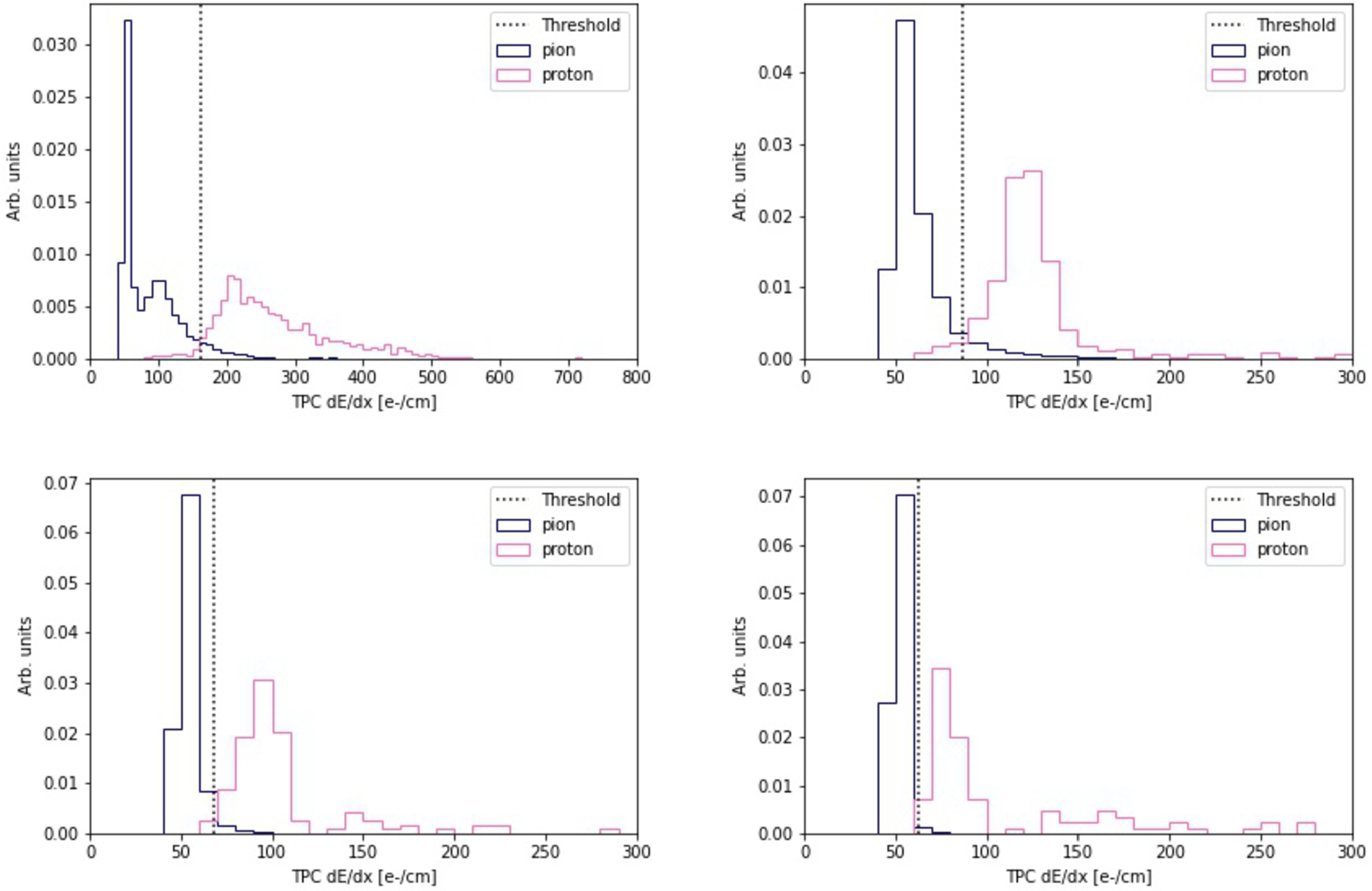
Fig. 63.
The distribution of the relationship between
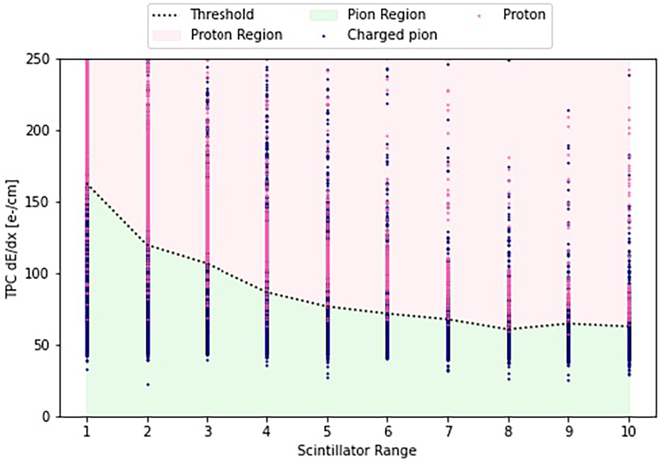
A more sophisticated approach is used for pion and proton discrimination. The energy loss per unit length (
Figure 63 illustrates the correlation between the TPC
A cut on the TPC
A discriminant region for the acceptance of pions and protons is delineated in Fig. 63. Specifically, a particle is classified as a proton if its
14.1.2.Neutral objects
Unassociated energy deposits in the calorimeter are grouped into clusters, designated as neutral entities. A subsequent pairing of these neutral objects is conducted for the purpose of invariant mass calculation. The invariant mass M between a pair of such entities is determined by Equation (17).
This methodology can be empirically validated through GEANT4 simulations by directing
The multiplicities of neutral and charged pions are key observables to characterise a signal-induced final state. The correlations between generated and detector-level multiplicities of charged and neutral pions and the total number of pions in each annihilation event are shown as normalised heat-maps in Fig. 65 and Fig. 66, respectively, for signal Monte Carlo-generated events described in Section 14.3. The yield of charged pions at the detector level typically replicates the true number of migration effects that can be seen. For example, some charged pions are lost through geometric limitations though this can compensated by an overestimation of the charged pion yield arises if, e.g. a proton or an electron or positron from a photon conversion is falsely identified as a pion. The detector-level neutral pion multiplicity suffers from a larger migration effect due to the requirement of finding two photons for each pion.
Table 6
The table provides an assessment of the particle identification efficiency within the experiment. Specifically, it quantifies the likelihood that a signal pion or proton is correctly classified or misclassified
| Truth particle type | ||
| Identified particle type | Proton | |
| 90.8% | 2% | |
| Proton | 9.2% | 98% |
Fig. 64.
Distribution of the diphoton invariant mass.
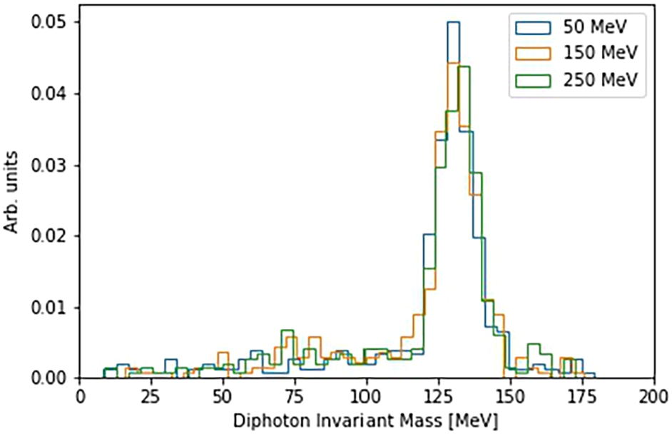
Fig. 65.
True and detector-level multiplicities for charged pions.
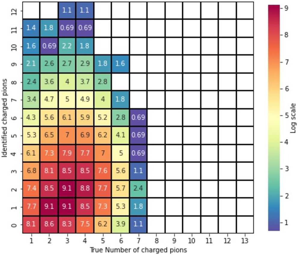
Fig. 66.
True and detector-level multiplicities for neutral pions.
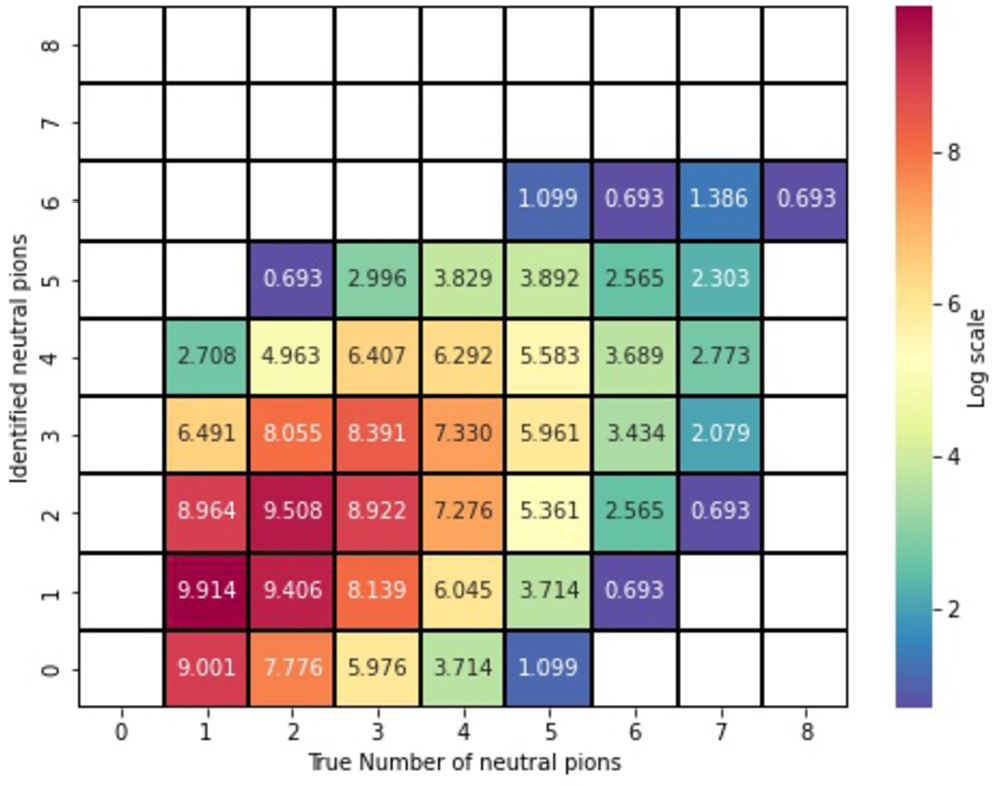
14.2.Vertex resolution
For most signal events, a vertex formed from charged particles emanating from the foil is expected. This is a strong discriminant between signal and backgrounds. Although a full track and vertex reconstruction is not available, the vertex resolution is dominantly determined by the 2 cm thick Al beam pipe. As a proxy for the expected vertex performance, an average weighted vertex position was estimated. The weight for each track is
Fig. 67.
The distance of closest approach
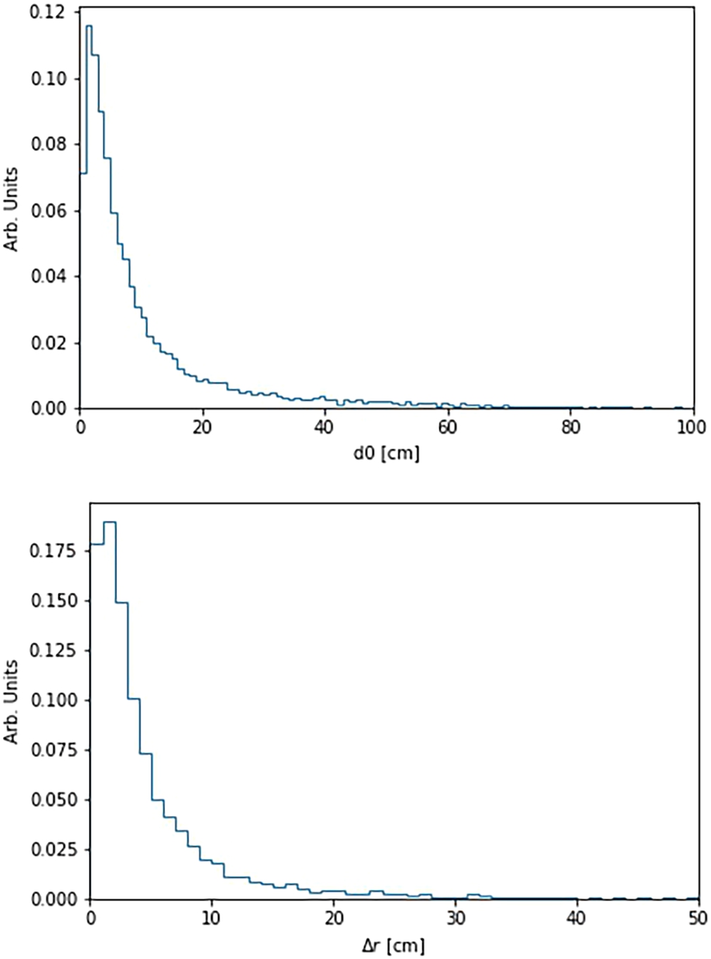
14.3.Signal
As described in Section 4.7, the post-annihilation final states were simulated using a stochastic intranuclear cascade model [50,106,107].
Figure 68 displays the distribution of kinetic energy of the final state interactions and scattering-related outgoing particles produced by the annihilation. Included are the decay products of heavy resonances. The energy of pions and photons can reach up to
Fig. 68.
The predicted distributions of the final state kinetic energies of outgoing annihilation-generated particles.
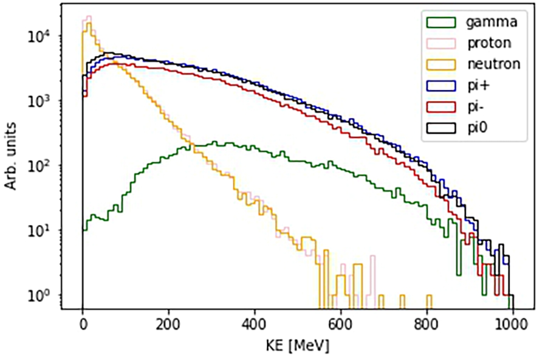
As mentioned in Section 4.7, due to final-state interactions invariant mass values significantly lower than two neutron masses are expected. This is illustrated in Fig. 69, which displays the initial and final invariant mass distributions of the annihilation process. Here, the “initial state” refers to the mesonic system formed immediately after the antineutron-nucleon annihilation, while the “final state” encompasses the system of pions and photons generated after considering nuclear effects and the decay of resonances. The extended section of the curve, where invariant mass values are low (≲1 GeV), is a consequence of meson absorption. Additionally, this curve takes into account photons produced as a result of resonance decays.
Figure 69 show the distribution of the total vector sum of momenta for pions. Even in the initial state, this distribution extends to high values due to Fermi motion and the attractive potential of the antinucleon, as explained in Reference [50]. In the final state, the tail of the total vector momentum, considering all pions and photons, becomes elongated. This effect is a result of both meson absorption and the decay of heavy resonances. It generally leads to a greater imbalance in the total vector momentum on an event-to-event basis within the mesonic system. Figure 69 also shows the relationship between the total momentum and invariant mass for both the initial and final states. The distribution in the final state highlights the significance of absorption and rescattering through final state interactions, particularly in predicting the post-annihilation invariant mass.
Fig. 69.
The initial and final state distributions of invariant mass (top left), the absolute value of the total momentum (top right), the relationship between the total momentum and invariant mass for the initial (bottom left) and final (bottom right) states.
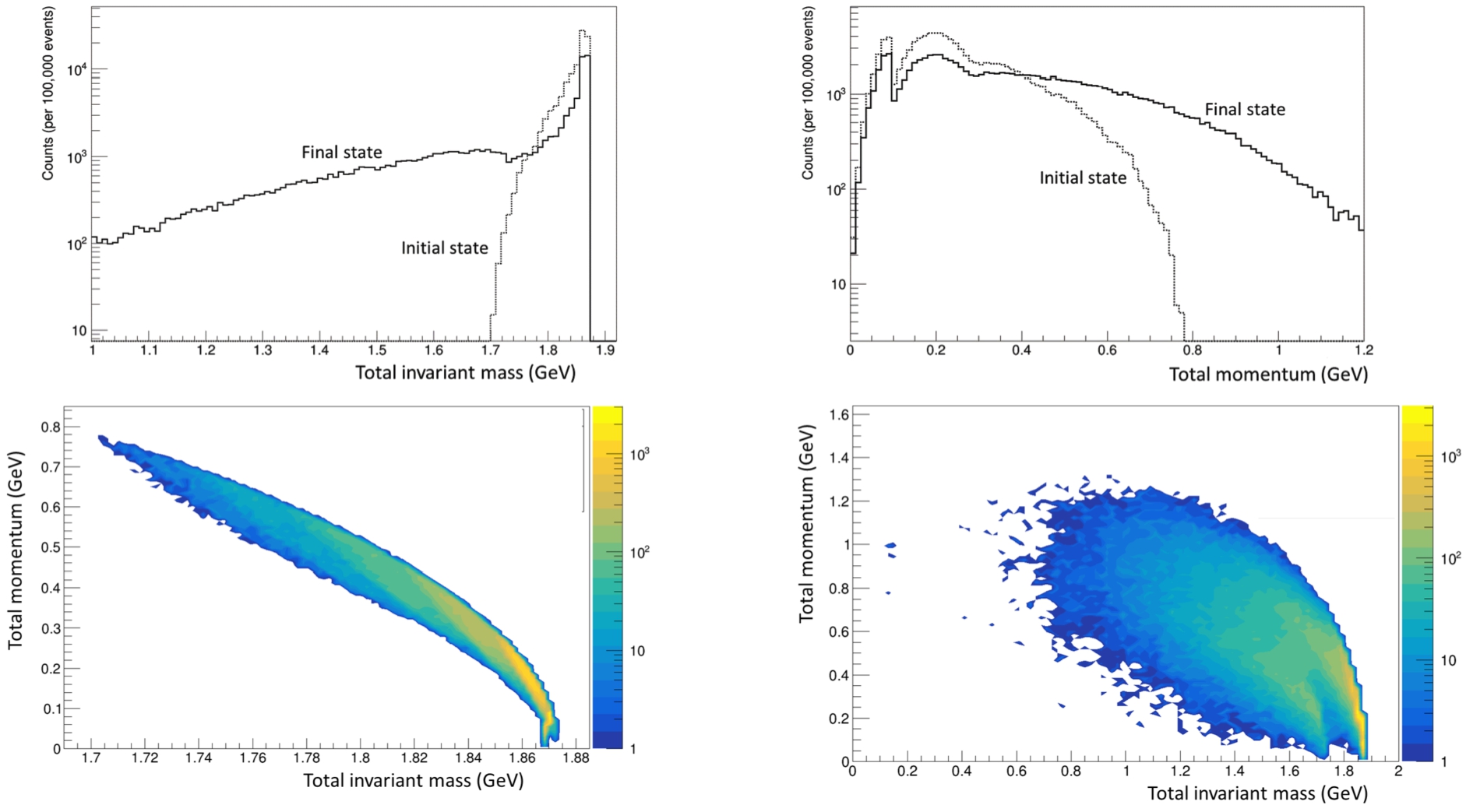
A sample of around 20,000 events were produced for a cold neutron flux focused over around 200 m onto the carbon foil.
14.4.Backgrounds
The principal background sources for the NNBAR experiment are expected to be cosmic rays and beam-generated backgrounds from the spallation source. As shown, the high energy spallation background can be excluded with a timing cut relative to the ESS clock. A key achievement of this work has to design a beamline satisfying safety specifications, demonstrating with MCNP calculations the evolution of the beam over 200 m and allowing the exclusion of fast neutron events with a timing cut. A timing cut can also handle skyshine, the remainder being suppressed with cosmic ray rejection selections. For cosmic rays, it is shown that a range of selections can be used to suppress the background. While the simulation samples do not statistically replicate the full sample expected for three years of running, the purpose of the study is to demonstrate that the experiment possesses a range of observables that would be used to reject cosmic ray events while retaining a high efficiency. As for other aspects of the NNBAR experiment, the pilot experiment, HIBEAM, is needed for data-driven sensitivity estimates.
14.4.1.High energy spallation background
The prompt particles from the spallation target include fast neutrons, protons, muons (from pion decays), and photons. These can have energies up to the GeV-scale can thus can potentially produce a pionic signature similar to that expected from a
Fig. 70.
The intensity of neutrons at the carbon target as a function of neutron energy (left) and time of arrival at the target (middle). The distribution of energy and arrival time is also shown (right).
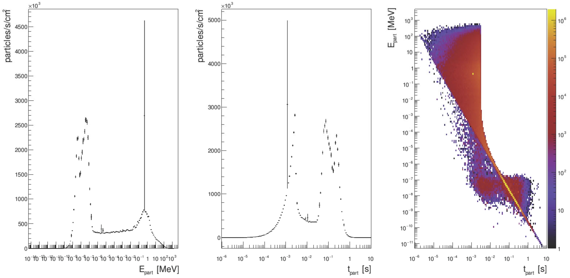
14.4.2.Skyshine
Skyshine [53,179] can be regarded as a fast neutron albedo from the atmosphere. Essentially, skyshine happens when an energetic neutron entirely escapes the facility through the shielding, scatters against the outside air, and returns to the detector region. A comparable term for particles that scatter against the earth is groundshine. Although the NNBAR detector is situated far from the tungsten target, skyshine can extend to several hundred metres. The fast neutron flux entering the atmosphere can be approximated with Equation (18).
The significance of skyshine in the context of the NNBAR experiment primarily stems from two key aspects. Firstly, it holds general relevance for any detector located at a spallation facility due to its capacity to disrupt detector electronics, leading to issues such as radiation-induced noise and single-event upsets. Secondly, skyshine has the potential to coincide with cosmic ray background events, making it imperative to predict the anticipated rate of these events.
Fig. 71.
Pareto chart of expected background contributions to generic long ESS instrument. Figure from reference [53].
![Pareto chart of expected background contributions to generic long ESS instrument. Figure from reference [53].](https://content.iospress.com:443/media/jnr/2023/25-3-4/jnr-25-3-4-jnr230951/jnr-25-jnr230951-g072.jpg)
In order to estimate the expected background contribution from skyshine we follow Reference [53], assuming no imperfections in the ESS construction for simplicity. Adding up the contributions from all sources including the banker wall, bunker roof, accelerator, target wall, and the so-called earthquake gap, we arrive at a rate of 44 n/s, as shown in Fig. 71. A detector response function of 0.1 is assumed for the instrument cave in Fig. 71, thus a raw external rate of 440 n/s can be assumed in the case of NNBAR. Since the NNBAR detector area is ∼180 m2, a total flux of 2–3 neutrons m−2s−1 is expected for NNBAR from skyshine background alone. It is a conservative estimation since it neglects the energy-dependent response function of the detector-shielding system for the NNBAR experiment. While the energy range of skyshine neutrons can extend to as high as ∼400 MeV, the background represents nothing more than a modest extra contribution to the cosmic ray background and as such, shall be treated using the same tools developed for it. There are of course differences between skyshine and cosmic ray background, in particular, due to having accelerator origin, skyshine background arrives at the detector region relatively soon (5–10 ms) with respect to the linac pulse, while cosmic ray events arrive randomly in time. This effectively means that part of the skyshine contribution is already being suppressed by the 5 ms timing cut to suppress fast neutron background, with the remaining contribution representing no extra challenge compared to cosmic ray background.
14.4.3.Cosmic ray background
The simulation of the expected cosmic particle flux over the detector is carried out using the Cosmic-ray Shower Library (CRY) [113] interfaced with the GEANT4 simulation. Cosmic particles are generated on a 24 m × 24 m event plane precisely above the detector and shielding complex. For each cosmic ray particle species, 20M events were simulated split over the different types of simulated cosmic particle for various energy regions. The flux of different cosmic ray backgrounds over the detector surface, sorted by energy ranges, are shown in Table 7. Table 8 shows the projected number of different cosmic ray backgrounds over the detector surface in 3 years of operation time.
Table 7
Simulated cosmic ray background flux at the detector using CRY. The data is sorted by ranges of kinetic energy (KE) and shown for various particle types
| KE (GeV) | Muon | Electron | Proton | Neutron | Gamma |
| 0–0.5 | 20.9 | 48.7 | 2.49 | 52.2 | 292 |
| 0.5–1 | 23.7 | 1.26 | 0.570 | 1.72 | 1.44 |
| 1–5 | 94.2 | 0.68 | 0.448 | 0.855 | 0.552 |
| 5–10 | 32.1 | 0.25 | 0.0202 | 0.0196 | 0.0139 |
| 10–50 | 25.3 | 0.0 | 0.0121 | 0.0105 | 0.00204 |
| >50 | 2.26 | 0.0 | 0.00810 | 0.000631 | 0.000150 |
Table 8
The expected number of incoming cosmic particles in 3 years of running time using CRY. The data are split into different ranges of kinetic energy (KE) and shown for various particle types
| KE (GeV) | Muon | Electron | Proton | Neutron | Gamma |
| 0–0.5 | |||||
| 0.5–1 | |||||
| 1–5 | |||||
| 5–10 | |||||
| 10–50 | 0.0 | ||||
| >50 | 0.0 |
14.5.Event selection and background discrimination
Event variables pertinent to the characterization of antineutron-nucleon annihilation events are elaborated upon in Reference [199]. In addition to the variables mentioned, timing window selection is also applied to hits registered in the calorimeter modules. A timing model has been developed to reject out-of-time hits and energy deposits from being used in the estimation of event variables.
The timing window for accepting hits arriving in the scintillator is defined by two key parameters: the time required for a charged pion to arrive at the center of a scintillator stave and a conservative treatment of the timing resolution. The window’s start time is calculated as
Likewise for lead glass modules, the timing window is determined by the time required for a photon to reach the module from the calculated vertex, represented as
Hits are accepted following the application of the timing window. Subsequently, event variables are computed based on the identified objects within the detector. These critical parameters include the multiplicity of charged and neutral pions, the invariant mass (W), and the sphericity (S) of the detected particle system. Another significant measure involves the total energy loss within the scintillator and lead glass modules.
The invariant mass of the hadronic system is calculated using Equation (19).
In this formulation, the index i enumerates the objects that have been identified in the detector. Each object’s mass is determined according to predefined criteria. The variable
The sphericity (S) of the detected particle system is computed with Equation (20).
Here,
Another pertinent variable under investigation is the filtered energy loss in the scintillator and lead glass modules, denoted as
A simulation study was conducted to illuminate the distribution of event variables for both annihilation signal and cosmic ray background events. The resulting distributions of invariant mass, sphericity, pion multiplicity, and filtered energies for signal and cosmic ray backgrounds are shown in Figs 72 to 76, respectively.
Fig. 72.
The distribution of invariant mass for signal and cosmic ray background events.
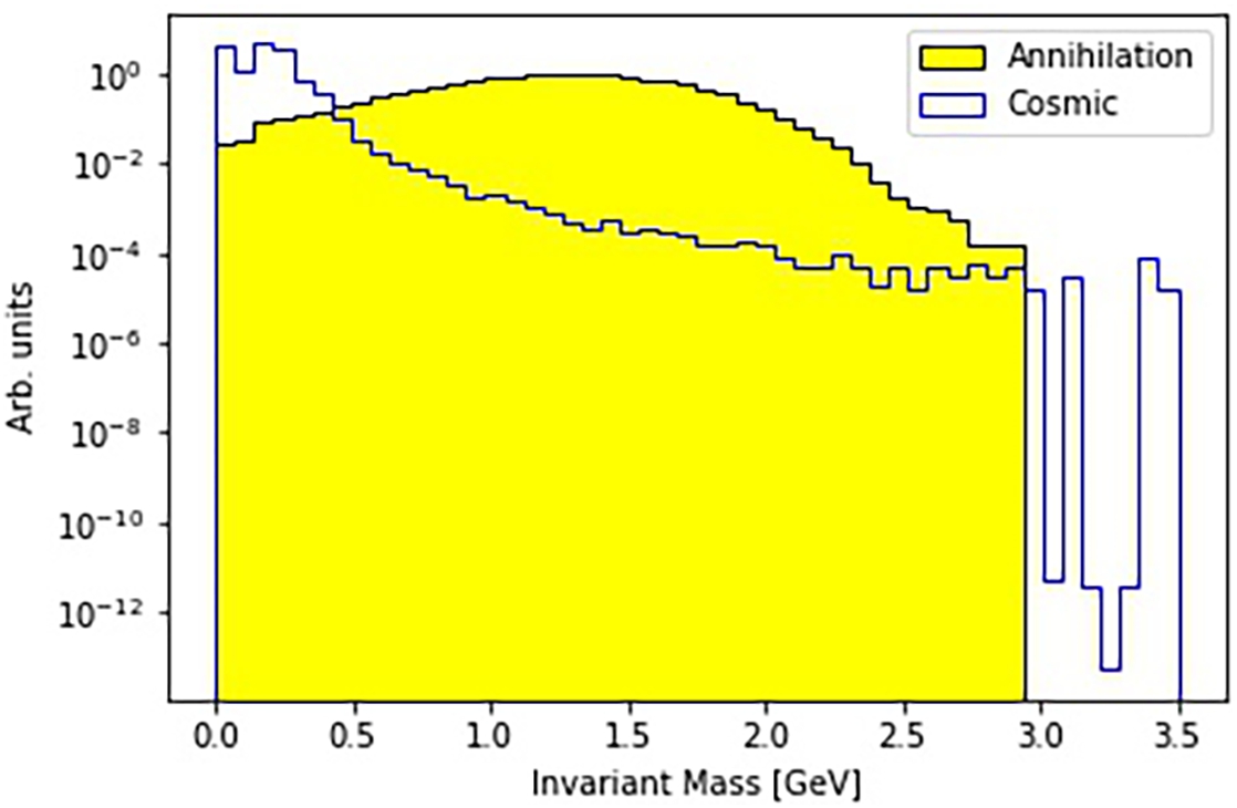
Fig. 73.
The distribution of sphericity for signal and cosmic ray background events.
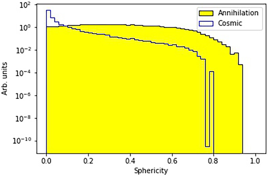
Fig. 74.
Number of pions identified in signal and cosmic ray background events.
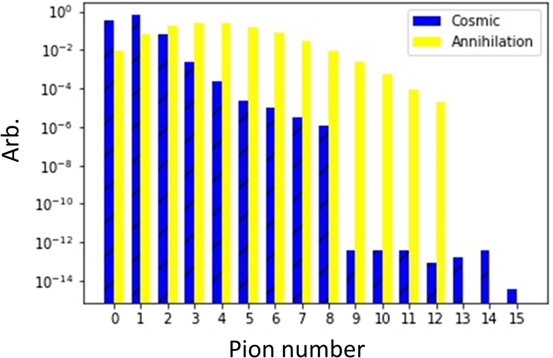
Fig. 75.
The out-of-time energy loss in the scintillators for signal and cosmic ray background events.
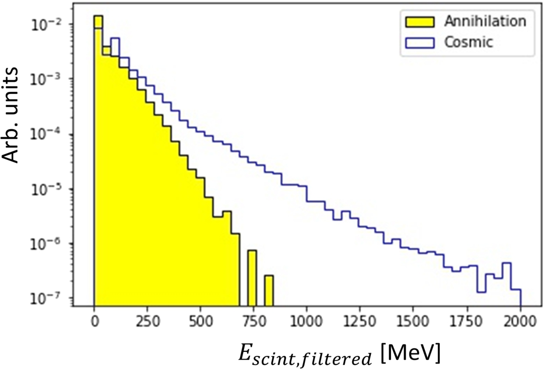
Fig. 76.
The out-of-time energy loss in the lead glass modules for signal and cosmic ray background events.
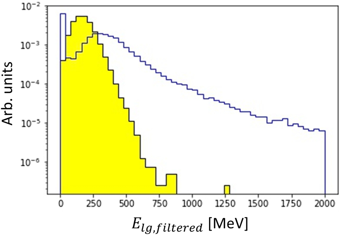
A preliminary scheme for discriminating between signal and background events is formulated based on the aforementioned event variables. The cutflow is organized as follows:
(1) The first layer of selections focuses on the scintillator modules. The total energy loss must fall within the range [
(2) The second layer, denoted as TPC track cut, mandates that at least one track be observed in the TPC. In addition, at least one track in the TPC must be traced back to the foil.
(3) The third layer necessitates the identification of at least one pion in the event, either charged or neutral.
(4) The fourth layer pertains to the invariant mass, which is required to exceed a predetermined threshold
(5) The fifth layer scrutinizes the sphericity of the event, which must be greater than a specific threshold
(6) The penultimate layer addresses the filtered energy loss in the scintillator modules, distinguishing between the upper modules with stave center
(7) The final layer of the cutflow has two components related to energy loss in the lead glass modules. Firstly, the energy loss occurring outside the pre-established timing window (
These layers of the cutflow aim to effectively separate signal events from background, particularly from high-energy cosmic ray events. The thresholds for each layer of the cutflow were globally optimized to achieve two principal objectives: to ensure that no cosmic ray background events survived the series of cuts for a maximal survival fraction of the signal events. As a result, the strategy effectively eliminates all cosmic ray background while retaining a substantial portion of the signal events.
The event survival rate subsequent to each layer of the cutflow with the globally optimized thresholds is tabulated in Table 9. The cutflow achieves a signal acceptance efficiency of 68%, while concurrently maintaining a 100% rejection efficiency (0 % acceptance) for cosmic ray background events. Since neutral cosmic ray particles as well as electrons and protons are overwhelmingly stopped by the concrete overburden, while high energetic muons are able to cross it, the background is split evenly between muon and non-muon background. The efficiency value of 68% is used for overall sensitivity calculations in Section 17.
The data in Table 9 do not include the active cosmic veto. A dedicated simulation was performed for this subsystem. A particle was assumed to be successfully vetoed when a number of photons equivalent to 10 keV energy deposition reached each of the 4 SiPMs of at least one scintillator stave. The result of this simulation is that >98% of the cosmic ray muons entering the active veto can be tagged and rejected.
As can be seen, full background rejection for the limited sample of cosmic ray events can be achieved. The purpose of this study is to demonstrate the availability of tools and observables which would be used to control the cosmic ray background level. The above was achieved with a minimal set of observables and a simple linear cutflow. The requirement of, e.g. a vertex would add yet more discriminating power. For the experiment, cosmic ray background would be monitored during non-data-taking periods. Furthermore, a second foil placed 20–30 cm downstream of the target foil would provide an estimate of the fake signal rates from cosmic ray events.
Table 9
Survival portion of annihilation signal events, cosmic ray background, and muon after each consecutive cut with globally optimized thresholds
| Selection | Signal | Non-muon background | Muon background |
| Scintillator energy loss | 0.89 | 0.008 | 0.3 |
| TPC track cut | 0.87 | ||
| Pion count | 0.82 | ||
| Invariant mass | 0.8 | ||
| Sphericity | 0.71 | ||
| 0.68 | - | - |
14.5.1.Cosmic ray interactions in the detector
The interactions of cosmic rays in the detector can give rise to fake signal vertices erroneously associated to the foil. A “danger zone” defined as a cylindrical region centered at the carbon target with a radius of
To assess the frequency and nature of such danger zone events in a three-year operational span of the detector, a dedicated study was conducted. Events were selected from cosmic ray background simulation samples, specifically those that exhibited interactions near the beam pipe. These events were then scrutinized for several key observables:
The expected number of particles traversing the carbon target.
The kinetic energy (KE) distribution of these particles.
The angle θ, defined as the angle between the particle momentum and the positive z-axis when hitting the carbon target.
Figure 77 and Fig. 78 show the KE and θ distributions of the particles passing through the carbon target. The y-axis represents the expected count of the particles over a 3-year operation period. Pions originating from cosmic events and passing through the carbon target tend to have kinetic energies that overlap with those of pions from the annihilation signal. However, the likelihood of observing such events remains low over the course of a 3-year operational period. The other particles primarily possess kinetic energies at the MeV or sub-MeV level, which may not be sufficient to produce a signal-like signature in the detector. None of these events are misclassified as signal events through our established event selection criteria.
Fig. 77.
The kinetic energy (KE) distribution of electrons, muons, pions, gammas, and nuclear fragments. The y-axis represents the expected counts of such particles within a given KE range over a three-year operational period.
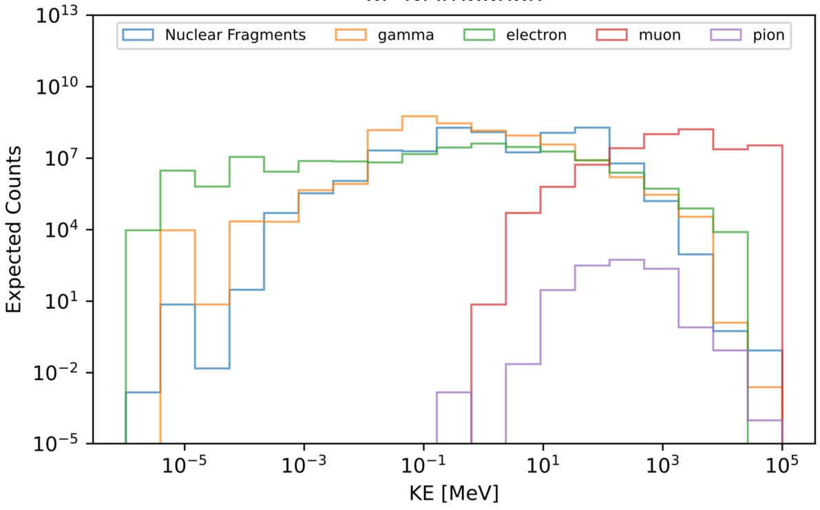
Fig. 78.
The θ distribution of electrons, muons, pions, gammas, and nuclear fragments. The y-axis represents the expected counts of such particles within a given θ range over a three-year operational period.
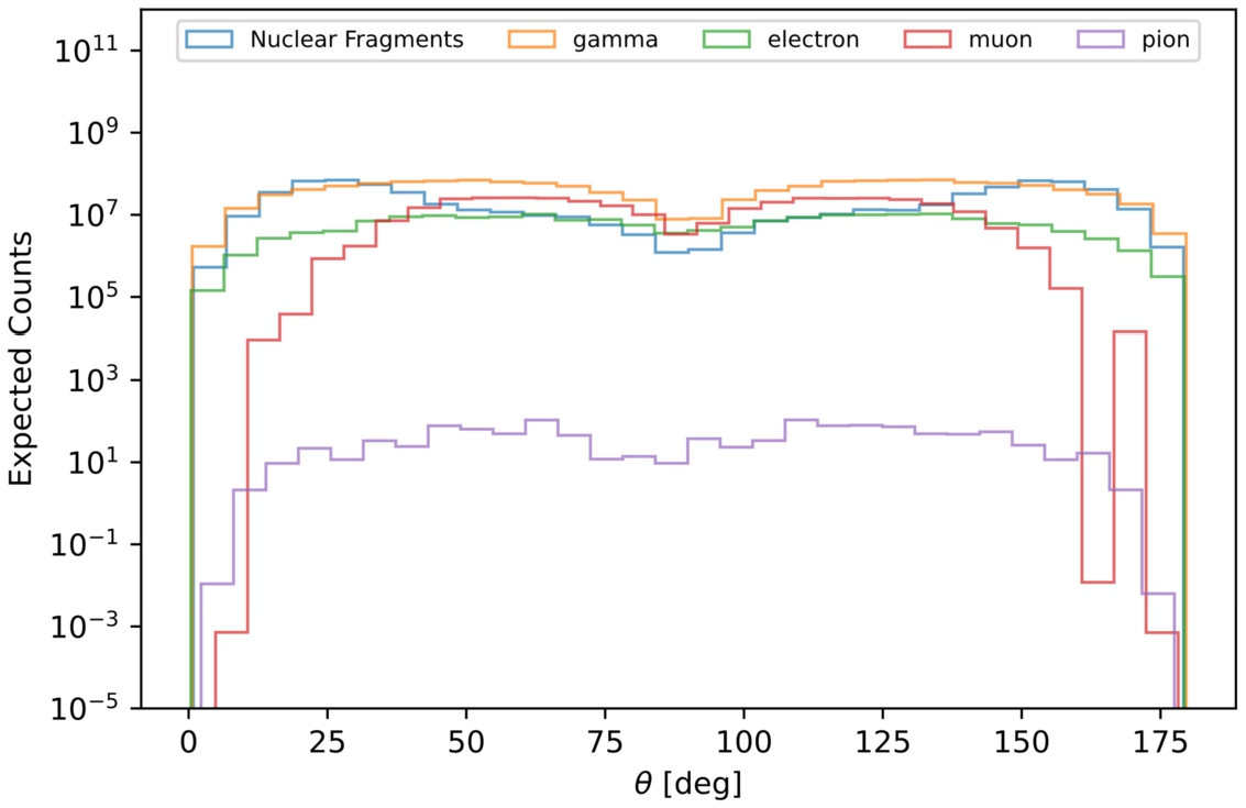
A principal focus of future work is the study of each type of interaction and how it can contribute to background.
14.5.2.Machine learning
Machine learning (ML) models were studied as an alternative event selection with respect to the linear cutflow.
Correlations. Correlation matrices were used to find any groups of variables and any independent variables. For a group of variables it holds that every variable is correlated to at least one other variable in said group. One correlation matrix was plotted for the signal and all background events respectively. The background events were categorized based on particle and energy range. The independent variables and groups from each correlation matrix was compared. The selected variables were deposited energy in the scintillators (Scint_eDep), longitudinal energy in the scintillators (Scint_E_L), difference in timing between the first and last hits in the lead glass and the scintillators, respectively, (Timing_lg and Scint_diff), longitudinal energy in the lead glass (Lead_glass_E_L), numbers of neutral pions based on loose and tight diphoton mass windows (pi0_loose_num and pi0_tight_num, respectively), sphericity, and invariant mass (Inv_mass).
Correlation matrices for signal and combined cosmic background are shown in Figs 79 and 80, respectively.
Fig. 79.
Correlation matrix for signal events.
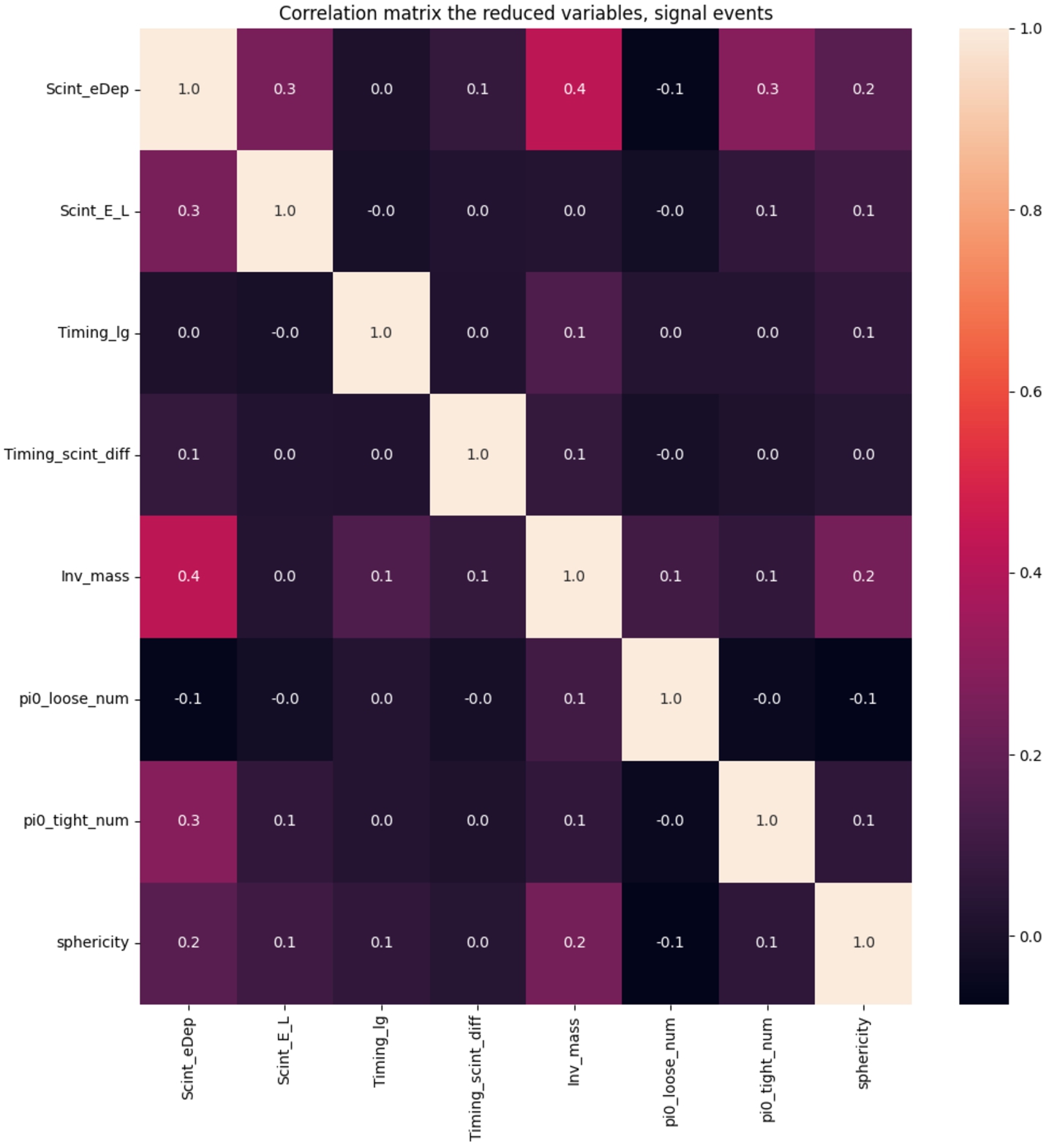
Fig. 80.
Correlation matrix for background events.
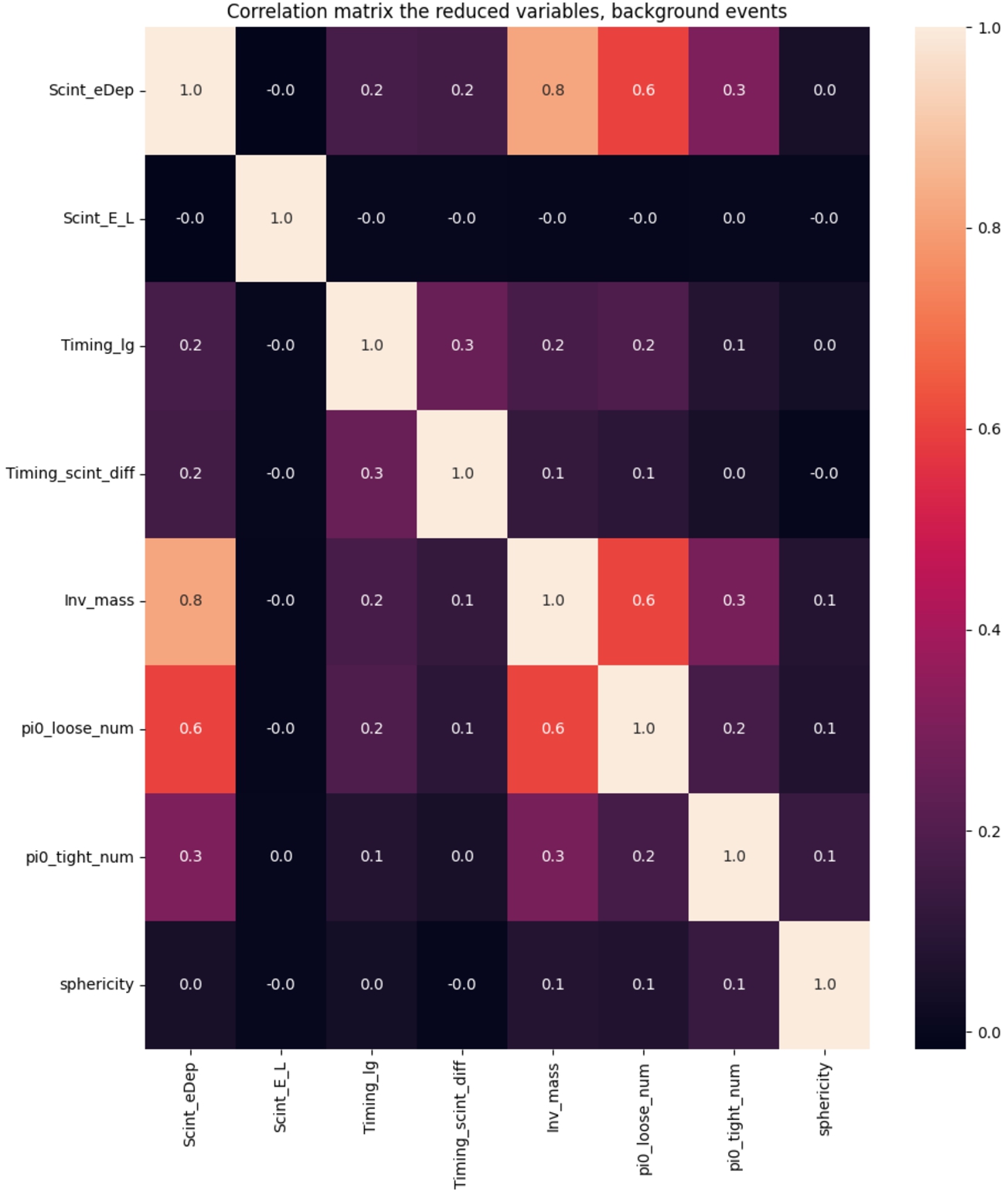
Suitable algorithms. In addition to standard selections, an option for selecting signal events at NNBAR whilst maintaining background rejection is to use ML. A number of algorithms were investigated, including Random Forest Classifier (RFC) [66], Boosted Decision Tree (BDT) [99] and Linear Discriminant Analysis (LDA) [120]. The algorithms were optimized using 20% of the signal After optimization of performance, tests for signal efficiency and background rejection showed that only the RFC was suitable for NNBAR. Precision Recall (PR) curves [149] were used to determine the skill of the RFC algorithm as well as to detect signs of overtraining [121].
Fig. 81.
Precision recall curve plotted for the RFC algorithm. The acronym auc stands for Area Under Curve. The f1-score is a measurement of a model’s accuracy. Note: none of the sets of validation data have been used for training or testing.
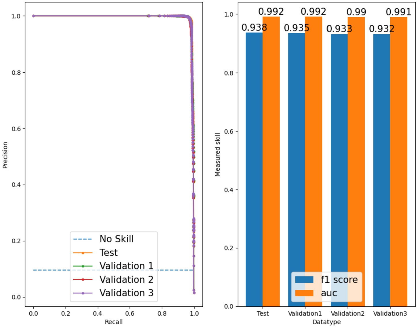
Results. The area under the PR curve serves as an indicator of skill. When this area approaches 1 for all datasets, it signifies a high level of skill. Conversely, significant variation in this area among different curves is indicative of overtraining. From Fig. 81 we see that the RFC is highly skilled and shows no signs of overtraining. The RFC provided 100% background rejection for all cosmic ray samples with a signal efficiency of 71%. A number of different sets of variables were used. The example above is chosen as it represents the most conservative estimate of signal efficiency obtained with full background rejection. The efficiencies for a range of sets of variables obtained range from around 70% to over 90%. The open question with ML is always how a decision is made and whether that decision depends on a difference in the simulation of signal and background that is not realistic. The ML should, therefore, be considered as an interesting and promising area for future study.
14.6.Comparison with the ILL experiment
When assessing the capability of the NNBAR experiment, a comparison should be made with the ILL experiment [43,44]. This experiment achieved a selection leading to zero background events using real data. In principle, from the point of view of cosmic ray background, as long as the number of calendar days for reaching the desired sensitivity is similar, the expected number of cosmic background should be of the same order of magnitude. The ILL experiment ran for a year. Since the NNBAR annihilation detector has, however, a larger area, the expected number of cosmic ray background events is, therefore, larger for NNBAR, with fluxes increasing by the proportion to which the NNBAR overall detector surface area is larger than ILL’s. Should background rejection in NNBAR be demonstrated to be quantitatively superior to ILL’s by at least this factor, zero cosmic ray background expectancy for NNBAR could be argued as a supplement to the detailed simulation-based work shown in Section 14.5.
Before comparing each background rejection factor it is thus necessary to compare the two annihilation detector sizes. The total surface of the ILL detector is ∼90 m2 [43], while the total surface area for NNBAR is around 180 m2. Thus, it must be demonstrated that, for the same data taking period length, that the NNBAR experiment has a background rejection that is superior to ILL by at least a factor of ∼2. Given that the NNBAR experiment would likely run three times longer than the ILL experiment, background rejection for NNBAR should be at least 6 times superior than achieved at the ILL.
A direct comparison between NNBAR and the ILL experiment with respect to cosmic ray background rejection is not straightforward, mostly because not all efficiencies to specific selections from the ILL paper are available. However, it is instructive to qualitatively compare the two detectors with respect to different background rejection capabilities, including, but not restricted to, timing, energy, as well as vertex reconstruction.
Generally speaking, timing capabilities of the NNBAR detector are far superior to those at the ILL. To first order this is simply caused by the fact that the NNBAR detector is larger and cosmic ray particles traversing the detector travel therefore longer distances making timing measurements, allowing the flight direction (inwards or outwards) to be determined. This gain is, however, further increased if one observes that not only is the scintillator system substantially more granulated with a multiple stave-based HRD, but that NNBAR’s electromagnetic calorimeter is also a timing sensitive detector to ∼ns precision. It takes ∼17 ns for cosmic ray particles to fully traverse the detector from top to bottom by making use of the lead glass time – a value which is significantly larger than the available resolution. The timing with lead glass will be useful for particles going outwards. The lead glass is partially “blind” to particles traveling inwards by using the directionality of Cherenkov light. If successful this would also help rejecting neutral cosmic ray events like e.g. gammas converting in the lead glass.
Moreover, particle identification for the NNBAR detector is in general far superior. In particular, the NNBAR detector can identify and reconstruct precision-time neutral signal pions while the ILL detector lacked a dedicated electromagnetic calorimeter.
Another important new capability of the NNBAR detector is that, due to NNBAR’s TPC, tracking in three dimensions is available which gives a significant gain in pattern recognition.
14.7.Pile-up
Background events producing a pionic signature and arising from beam interactions on the foil or beam wall arise from fast neutrons that can be excluded with timing selections. Low energy neutrons and their interactions can contribute a sea of low energy particles, largely at the MeV-scale and below. These are dominantly photons and electrons. Neutrons at the eV-scale and below can also enter the detector.
The flux of particles causing beam-induced noise depends critically on the optimization of beamline around the detector, including recesses, endcap locations, and the choice of type and location of moderator materials and neutron poisons. The optimization of the beamline is a focus area for future work. However, some early MCNP calculations have been made with the unoptimized “worst-case” beamline in the detector area (Section 8, around which it is instructive to discuss the issue of beam-induced noise in the detector77). Unlike the GEANT4 studies, the calculations were made with a coarse-grained detector model in which each component was replaced with a slab of appropriate material. Layers of 6LiF and polystyrene of thickness 0.5 cm were placed inside the beam pipe in the beamline area as a basic neutron poison88 and moderator, respectively.
It should first be noted that there will be an irreducible photon background of the order of
Threshold cuts are a key tool to study and suppress pile-up in the scintillator arrays owing to the weaker signal left by MeV-scale pile-up particles compared to the ∼10 MeV left by signal particles in 3 cm of scintillator. However, the absence of a magnetic field in the TPC implies that Compton electrons will appear as tracks.
Table 10
Estimated flux of particles entering different detector subsystems
| Component | Flux | ||
| n | γ | ||
| TPC | |||
| Scintillator layer 1 | |||
| Scintillator layer 2 | |||
| Lead glass | |||
Table 10 shows the flux of particles in the slow neutron window of (i.e. after the 5 ms timing cut described in Section 14.4.1) entering the different subsystems as estimated with MCNP simulations. For the TPC, ALICE-like conditions may be expected of around 650 tracks per 50 ns window, likely necessitating additional scintillators before the TPC to remove timing and track reconstruction ambiguities. The tracks themselves will largely be entering the TPC from random directions. This also requires a dedicated effort for track reconstruction in this high multiplicity environment and the linking of tracks to groups of staves to identify pion tracks from low energy beam-induced particles.
Without the electron background tracks, a traditional TPC with wire chamber readout could be used, even without gated operation. However, the large number of tracks per second due to electron background implies that the issue of the ion backflow from the avalanche region must be addressed. The problem has already been solved by the ALICE TPC upgrade by using GEM instead of multiwire proportional chamber (MWPC) readout. Without gating it will then also be possible to use the TPC in continuous readout mode (i.e. none or very loose hardware trigger).
It should again be emphasised that the fluxes in Table 10 represent the unoptimized beamline in the detector area. An earlier study was made with GEANT4 using incoming slow neutrons. This gave fluxes several orders of magnitude lower than in Table 10. However, a different beamline design around the detector area was assumed. A full determination of the beam-induced noise requires an optimization of the beamline together with the identification and mitigation of sources of large particle fluxes. Predictions from different radiation transport models must be validated against each other and, ultimately, prototype test data. The issue of pile-up and its possible influence on the detector design is discussed in Section 19.3.
15.DAQ for the NNBAR experiment
The NNBAR data acquisition system must trigger on and read out detector signals with sufficiently precise timing, energy and spatial resolution to effectively discriminate between neutron–antineutron annihilation candidate events and unrelated backgrounds. Balancing this requirement is the need to reduce readout of manageable bandwidth levels and thus avoid dead time.
Table 11 summarizes the estimated channel numbers and readout parameters of the four main NNBAR Subdetectors. Three of them, namely the HRD, LEC and cosmic veto, are “fast” scintillator/Cherenkov detectors with SiPM readout that can measure energy and precise (∼ns level) timing information with low readout latency. The timing precision from these subdetectors is critical for signal/background discrimination, as well as for reading out and matching data from track candidates in the TPC. Since TPC tracks have drift times as high as 100 μs, the baseline NNBAR DAQ design first identifies initial events and track candidates from the “fast” subdetector data, and then adds selected TPC data to the event for track matching, either in the real-time event builder or offline.
The HRD, LEC and veto detector front-end electronics are read out by fast SiPMs, allowing a high degree of commonality between the front-end electronics, digitization and readout between the combined ∼40,000 SiPM channels across the three systems. Collected scintillation/Cherenkov light is converted to fast pulses by SiPMs. The SiPM pulses are then transformed by preamplifier/shaper circuits into analog pulses with amplitude-independent shape and at least 50 ns rise time, which are then continuously digitized at 80 MHz by an on-detector digitizer and readout system based on commercial ADCs read out by programmable logic devices (FPGA). Finite-impulse-response (FIR) filters will allow both amplitude and ∼1 ns precision timing extraction from the digitized data.
The baseline TPC readout is designed around the SAMPA ASIC, which was designed for the ALICE TPC and muon chamber upgrades at LHC. SAMPA is a 32-channel mixed-signal IC that combines pre-amplification, shaping and digitization, as well as a DSP layer that can be used to apply baseline correction and data compression before reading out the processed data in multiple serial data streams. The SAMPA chip allows triggered readout of zero-suppressed data within programmable-length data frames with up to 10 μs latency, which may be used to limit TPC readout to time frames associated with candidate events seen in the calorimeters. If background rates are high, the TPC can also be read out in continuous mode.
Table 11
Subdetector channel count and data size
| Detector | Channels | Dynamic range | Data size | Readout |
| TPC | 256k channels | 10 bits | - | Continuous |
| HRD | 9000 SiPMs | 10–12 bits | 200 bytes | Self-triggered |
| LEC | 32000 SiPM arrays | 10–12 bits | 200 bytes | Self-triggered |
| Veto | 1000 SiPMs | 10 bits | 200 bytes | Self-triggered |
A conceptual layout of the NNBAR DAQ system is shown in Fig. 82. As mentioned above, candidate events and track candidates will be initially identified by the “fast” HRD, LEC and veto subdetectors. Unlike at collider experiments where signal events are time-aligned with particle bunch crossings, signals and backgrounds in NNBAR will have arbitrary timing, with the additional complication that the flight times and angles of annihilation event products will vary with the vertex position at the target. Therefore, candidate event selection with rejection of unrelated backgrounds requires the absolute timing of particle hits in the fast detectors to be measured with nanosecond or better precision, and a CPU-based trigger/event-builder farm for event candidate selection and reconstruction. Data reduction to the CPU-based trigger is achieved through self-triggered (a.k.a. “triggerless”) readout of fast detector pulses from individual channels, with time stamps included with the digitized pulse data. Initial event selection in the trigger begins with topology and timing-based algorithms from the calorimeter and veto data, with later addition of selected TPC data for the final event selection and reconstruction.
Fig. 82.
Conceptual overview of the baseline NNBAR DAQ.
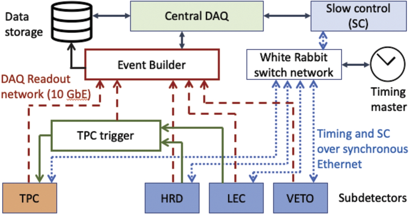
Event selection in the NNBAR trigger will be primarily based on detected hits in the HRD, LEC, and the veto detector. A preliminary signal trigger definition would include a minimum combination of minimum-ionizing “tracks” through multiple layers of staves (a proxy for charged pions) and spatially separated clusters of lead glass deposits over a given threshold (a proxy for charged pions), with cosmic muon rejection provided by timing and spatial hit data from the veto detector. At the ILL experiment the majority of triggers (2.4 Hz out of 4 Hz), were caused by cosmic muons traversing the detector without triggering the veto. We expect a similar order of magnitude of contribution for the NNBAR trigger, and therefore estimate that the signal trigger rate of NNBAR will also be on the order of a few Hz.
15.1.Front-end system
The baseline solution for global timing distribution at NNBAR is the open-source White Rabbit technology, which has been developed at CERN for distributing sub-nanosecond timing distribution over synchronous Ethernet. White rabbit was initially developed for timing and control, and the conceptual design shown includes a White Rabbit switch network connecting the global timing master and the detector slow-control system with the sub different subdetector systems over gigabit Ethernet links.
While White Rabbit can in principle also be used for general purpose data transfer, this imposes some overheads that can be avoided by instead using separate networks for timing and control (GbE) and readout to the event builder (10GbE), with the latter system comprised of commercial CPUs and network switches.
The self-triggered readout architecture for the calorimeter and veto systems begins with the FPGA-based front-end digitization modules. Sampled data from each channel are locally monitored, and when a valid pulse above a set threshold is identified, the module autonomously transmits the channel data to the off-detector systems for reconstruction and triggering. Since only detected pulses are read out, the total readout bandwidth for the calorimeter and veto systems is highly zero-suppressed. The transmitted data contents will include a time-stamp aligned to a global master clock, as well as the digitized pulse data (typically 10–12 samples) and any additional required information such as checksums and/or status bits. The expected total read out data for a detector pulse is approximately 200 bits, and will be encapsulated into Ethernet packet format by the FPGAs for direct transmission from the digitization system to the event builder farm.
The calorimeter/veto digitization modules are foreseen to be installed in ATCA-type crates equipped with dual-star topology backplanes. To reduce the number of optical links required, one of the star network hubs will contain a network switch that can read out data from up to 12 modules over a single 10 GbE link per crate. The second star hub would contain a timing and control module for distributing timing and control signals received from a White Rabbit GbE link.
For the TPC readout, the baseline design in this report assumes pessimistic background estimates and large track multiplicities. In this scenario the SAMPA chips are read out in continuous mode with no zero suppression, over optical fiber links with 4.8 Gbps line rates. The TPC links are received off-detector by FPGA-based boards comparable in design and function to the Common Readout Unit (CRU) developed for the high-luminosity upgrade of ALICE. These boards process and reduce the TPC data (including zero suppression as needed), and then transmit them as Ethernet packets over 10 GbE links to the event builder.
In the event that zero-suppression is insufficient for TPC data reduction, a hardware-based TPC trigger is foreseen that would combine hit data from the HRD and LEC to identify potential particle candidates arriving from the direction of the target, and trigger selective readout of the TPC channels corresponding to the volume through which the track candidate would have passed. The TPC trigger would receive fixed-latency “hit” signals from the front-end digitization and readout modules for the HRD and LEC, and perform FPGA-based topology algorithms. Particle track candidates identified by the TPC trigger would also be included in the event builder readout to help match the TPC data with the relevant events.
15.2.Event builder
Readout from the calorimeters, veto and TPC systems are transmitted off-detector over optical links to the event builder system, where they are distributed through a network of high-capacity ethernet switches to rack-mounted high-performance computing nodes.
A relatively small portion of the computing nodes will perform the initial trigger selection from the HRD, LEC and veto data. Because the readout links from these detectors are sparsely populated, off-detector network switches will further concentrate the data into a smaller number of these nodes. The average event sizes in the calorimeters and veto are expected to be small, in the range of a few kB within a given time interval, and the initial event selection will use relatively simple trigger algorithms such as FIR filters for extracting pulse amplitude and fine timing, and simple event topology calculations based on selection based on the timing and position of detector hits.
The largest portion of the event builder resources is dedicated to readout of the TPC data, which are concentrated by high-performance switches into a significant number of densely populated 100 GbE links for distribution to the computing nodes. After an event candidate has been identified in the initial trigger selection, the corresponding TPC data are extracted and added to the event record. If TPC background rates and computing node resources allow, the online reconstruction stage of the event builder may include operations like vertex reconstruction, track matching to calorimeter hits and/or further zero-suppression of the TPC data. Otherwise, the event builder may in principle simply read out the corresponding TPC track data and send it to mass storage for further analysis offline.
15.3.Radiation tolerance
The NNBAR detector and front-end electronics systems will be exposed to multiple sources of radiation, including scattered beam neutrons as well as secondary particles from neutron interactions with the target and detector. The TPC front-end electronics are based on radiation-hard ICs developed for much more challenging radiation conditions at LHC/ALICE. On the other hand, the baseline HRD and LEC on-detector systems are planned to use commercial components, so it is important to consider whether such systems will withstand the radiation exposure over the planned 3 years of NNBAR data taking.
Initial estimates of ionizing (TID) and non-ionizing (NIEL) radiation exposure to the detectors and front-end electronics exposure have been produced from detector background simulations using MCNP (see Section 14.7), and are summarized in Table 12.
Table 12
Estimated annual ionizing (TID) and non-ionizing (NIEL) radiation exposure for the NNBAR detectors and their front-end electronics. The TPC and HRD electronics dose rates vary depending on their position upstream or downstream of the target
| Detector | TID (Gy/yr) | NIEL (1 MeV equiv. |
| TPC | 71 | |
| TPC electronics | 14–23 | 2.0–3.2 × |
| Scint. staves (HRD) | 23 | |
| HRD electronics | 8–33 | 5.3–5.6 × |
| LEC | 3 | |
| LEC electronics | 0.3 |
For comparison, the estimated 10-year TID and NIEL doses for the high-luminosity upgrade of the ATLAS hadronic Tile Calorimeter front-end electronics are 22 Gy and
It should be noted that the most radiation sensitive components in the HRD and LEC on-detector electronics will be the FPGAs and other complex digital circuits in the digitization and readout modules. These will be installed outside the LEC, where the TID and NIEL rates will be substantially lower than at the HRD front-end boards.
We therefore conclude that HRD and LEC front-end electronics and on-detector digitization/readout systems will operate in conditions that are compatible with use of radiation-qualified commercial components. Single event effects in the FPGAs will be mitigated with standard methods including triple-mode redundant logic, configuration memory scrubbing, and checksum-protected data readout.
16.Mechanical structure of the NNBAR detector
An early draft design for the baseline NNBAR detector mechanics and support structure has been produced. The main goals of this exercise were to demonstrate that a realistic support structure for the NNBAR subdetectors can be built with a feasible installation plan, while avoiding excessive dead material in the active detector volume that would degrade the detector performance.
16.1.Support structure
Assembly of the annihilation detector begins with construction of a large structure (Fig. 83) for supporting the various detector elements and distributing the detector weight evenly across the floor of the experimental hall. A heavy structure of double-T steel beams supports the HRD and LEC calorimeters as well as other service structures such as working platforms, stairs electronics racks, and so forth. An inner framework of aluminum provides a support structure for the TPC and beam tube with minimal dead material.
The steel support structure weighs approximately 40 tons and is designed to support a full annihilation detector weight of nearly 200 tons. The top-most beams are omitted during the early installation stages to allow access for the innermost detector components, and added later for installation of the top-most HRD layers and the LEC.
Fig. 83.
Left: the steel and aluminum NNBAR detector support structure with movable support points for installation of the central beam tube. Right: beam tube installation.
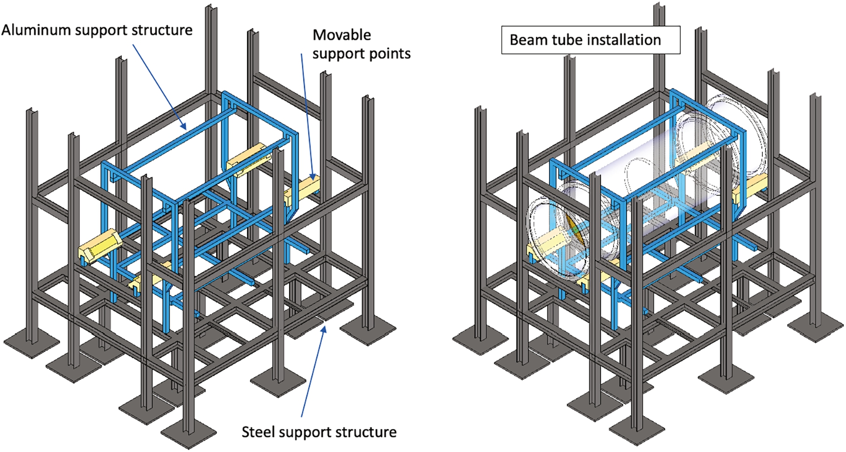
16.2.Beam tube
The central beam tube is approximately 6.5 meters long and weighs ca. 3.7 tons. Two circular ribs at each end of the tube provide rigidity to prevent the tube from deforming under its own weight. The ribs also serve as mounting points for four sliding supports used during the tube installation process.
16.3.TPC installation
The TPC is also supported by the aluminum frame surrounding the beam tube. To reduce dead material, the TPC chambers can be fixated together to create a more self-supporting structure with a total weight of 600 kg.
16.4.HRD installation
The HRD is pre-assembled in large 10-layer planar sections before transport and installation in the experiment hall. Since the outer edges of the HRD planes are instrumented with SiPMs and front-end boards, assembly and mounting of the HRD sections will require fasteners that pass through the stave structure at regular intervals to aluminum profiles as illustrated in Fig. 84. This would necessitate small gaps in the stave structure, but the expected impact on HRD coverage would be negligible.
The total weight of the HRD is estimated at 29 tons.
16.5.LEC installation
The LEC is the largest and heaviest subdetector, with more than 32000 lead glass counters and a total assembled weight of nearly 100 tons. To facilitate installation a commercial “slide guide” system of extruded aluminum profiles would support pre-assembled modular blocks of 9 lead glass counters in a
Fig. 84.
Clockwise from left: TPC installation around the central beam tube, with an HRD section below; a hanging HRD section with aluminum supports; LEC installation detail with modular assemblies of 9 counters each mounted on aluminum slide-guide profiles.
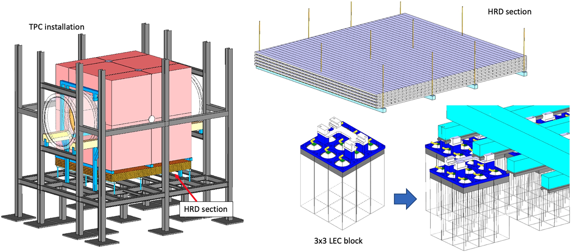
16.6.Working platforms and stairs
The annihilation detector design also includes working platforms and stairs to allow safe access to all parts of the detector for installation and maintenance work (Fig. 85).
Fig. 85.
Working platforms and stairs in the experimental hall.
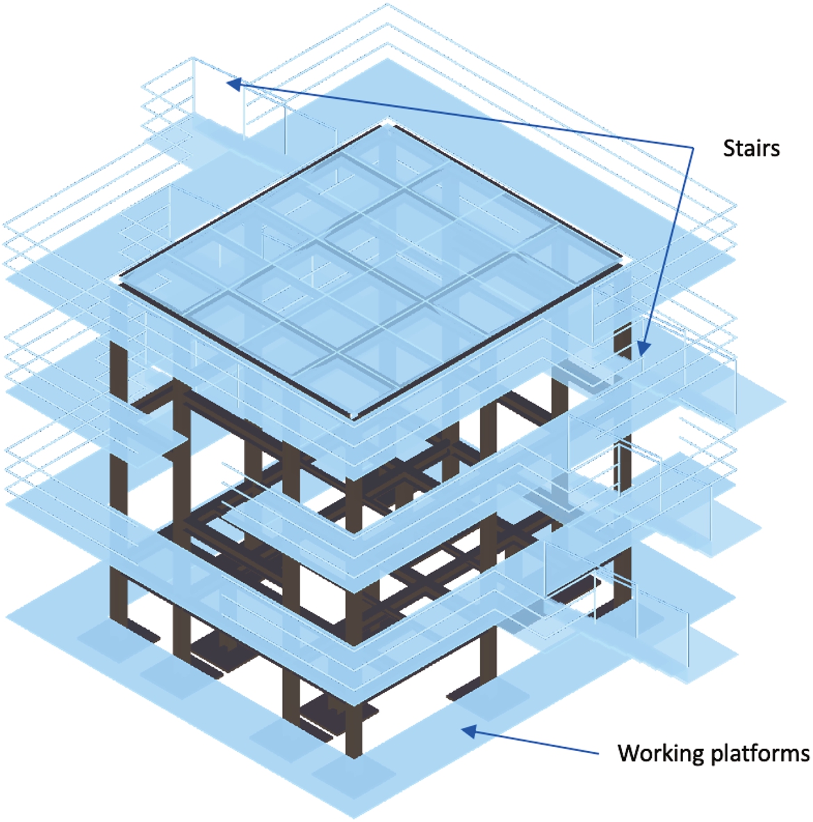
16.6.1.Shielding and veto
The cosmic veto system is mounted on the concrete shielding walls surrounding the annihilation detector.
17.Sensitivity of the experiment
The sensitivity (FOM and
(1) The ESS accelerator power. Two scenarios are considered: 2 MW and 5 MW. As shown in Section 2 of Reference [161], the differences in shapes of neutron spectra from the
(2) The optics and beamline configuration. For an accelerator power of 2 MW and a monoplanar reflector deployed around 17 m from the bunker followed by a square-shaped tube section which transitions to a circular cross-section after 20 m, the FOM is 300 ILL units per year (Section 10.9.2).
(3) The background level. As shown in Section 13, a timing selection of at least 5 ms after the proton beam hits the tungsten target will suppress high energy spallation background. Given the ESS repetition rate of 14 Hz, this corresponds to an acceptance of
(4) The extent to which the quasi-free condition is maintained. Neutrons propagate through a low but not zero field region (Section 11). A Monte Carlo study stepping slow neutrons through the simulated field, and evaluating the cumulative effect of average values of a non-zero magnetic field at each position, showed that the quasi-free efficiency is around 98–99%. Analytical calculations of the departure from the quasi-free conditions for fields of the size in NNBAR imply an inefficiency of around 5% for a 200 m magnetically shielded length [84]. An efficiency of
(5) Operation time. The ILL experiment ran for one year. It is anticipated that NNBAR would operate for at least three years.
An enhanced definition of the FOM (
The sensitivity to the
Fig. 86.
Limits from searches with bound neutrons (blue circles) and free neutrons (red circles) and the sensitivity of the future DUNE (blue triangle) experiment. The sensitivities of the NNBAR experiment at 2 MW and 5 MW for a zero background search are also shown (red triangles).
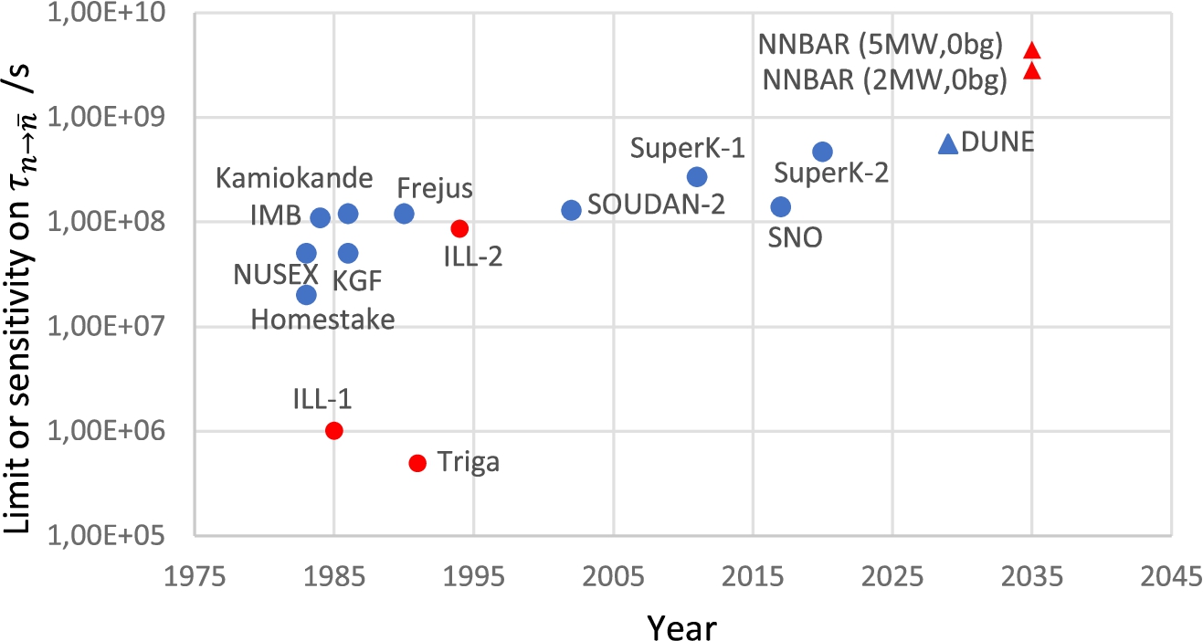
Table 13
Cost breakdown of an instrument with the baseline specifications, i.e. length = 200 m,
| Item | Cost (M €) |
| Carbon target | 0.07 |
| Vacuum tube | 4.76 |
| Vacuum system | 9.0 |
| Magnetic shielding | 5.5 |
| Steel shielding | 3.05 |
| Beam tube concrete shielding | 11.07 |
| Detector cave concrete shielding | 1.42 |
| Detector mechanical construction | 0.75 |
| Counting house | 0.03 |
| Beamstop | 4.78 |
| TPC and front-end electronics | 3.53 |
| TPC readout to DAQ | 1.94 |
| Lead glass | 7.07 |
| Lead glass SiPM and analog front-end | 13.60 |
| Stave scintillators | 0.12 |
| Stave SiPM and analog front-end | 0.46 |
| Stave WLS | 0.36 |
| Veto scintillators | 0.07 |
| Veto WLS | 0.19 |
| Veto SiPM and analog front-end | 0.38 |
| Calorimeter/Veto digitization and readout | 2.11 |
| Timing and slow control | 0.19 |
| DAQ system | 2.11 |
| Optical elements | 5.10 |
| Total | 77.66 |
The above sensitivities correspond to a baseline of a 2 m diameter beamline in the detector area with the costing given in Table 13. As shown in Section 18, variations in the diameter, while also maintaining the same detector acceptance, can enhance or degrade the FOM.
It should be emphasised that the relevant quantity when considering the capability of a search for free neutrons converting to antineutrons is the ability of the experiment to observe such a process. This is directly proportional to the figures of merit discussed here and is thus the relevant quantity to show an experiment’s discovery potential.
As an indication of the ability of NNBAR to test theories of physics beyond the SM, Fig. 87 shows the likelihood distribution of oscillation times in a baryogenesis (PSB) scenario (see Section 4.3). As can be seen, the NNBAR experiment is sensitive to a larger parameter space than was previously available.
Fig. 87.
Likelihood distribution for neutron–antineutron oscillation time for a PSB scenario. The limit from Super-Kamiokande (SuperK-2) [6] is shown as are projected oscillation time sensitivities and exclusions for a zero background NNBAR experiment for accelerator power scenarios of 2 MW and 5 MW. Figure adapted from reference [36].
![Likelihood distribution for neutron–antineutron oscillation time for a PSB scenario. The limit from Super-Kamiokande (SuperK-2) [6] is shown as are projected oscillation time sensitivities and exclusions for a zero background NNBAR experiment for accelerator power scenarios of 2 MW and 5 MW. Figure adapted from reference [36].](https://content.iospress.com:443/media/jnr/2023/25-3-4/jnr-25-3-4-jnr230951/jnr-25-jnr230951-g088.jpg)
Figure 88 shows the oscillation time versus the scale for new physics in a R-parity violating supersymmetry scenario (see Section 4.5). The NNBAR experiment extends sensitivity to a mass scale of new physics by up to around 400 TeV and can probe the PeV scale.
Fig. 88.
Relationship between the oscillation time and the mass scale for new physics in a R-parity violating supersymmetry scenario. The calculations are presented using the best estimate for the matrix element together with two predictions corresponding to shifting the matrix element according to uncertainties thus forming an envelope around the central estimate. The limit on oscillation time from searches at the ILL (ILL-1994) [44] and Super-Kamiokande (SuperK-2) [6] are shown together with oscillation time sensitivities a zero background NNBAR experiment for ESS accelerator power scenarios of 2 MW and 5 MW. Figure adapted from reference [74].
![Relationship between the oscillation time and the mass scale for new physics in a R-parity violating supersymmetry scenario. The calculations are presented using the best estimate for the matrix element together with two predictions corresponding to shifting the matrix element according to uncertainties thus forming an envelope around the central estimate. The limit on oscillation time from searches at the ILL (ILL-1994) [44] and Super-Kamiokande (SuperK-2) [6] are shown together with oscillation time sensitivities a zero background NNBAR experiment for ESS accelerator power scenarios of 2 MW and 5 MW. Figure adapted from reference [74].](https://content.iospress.com:443/media/jnr/2023/25-3-4/jnr-25-3-4-jnr230951/jnr-25-jnr230951-g089.jpg)
18.Cost estimation of the experiment
In addition to the usual spreadsheet-based costing breakdown that one would typically use for a project of this scale, a parametric study was performed to understand the cost-benefit curves in part of the effort to arrive at a baseline specification. This study was based on a costing tool developed in python at the ESS for regular neutron experiments, in order to establish the correct strategy to maximise return on investment in instrumentation [54].
The original software used manufacturer quotes from 2013 for all the major components of a “normal” neutron instrument and was heavily benchmarked against other neutron facilities around the world. Those generic functions were then adapted specifically for the work on NNBAR in the current project, including the specialised detector technology that is needed. The construction of the ESS has allowed the refinement of a number of engineering and materials costs since 2013, and these were updated. Finally, a more recent quote was obtained from a neutron optics vendor, which takes into account recent economic changes since 2013, along with improvements in manufacturing efficiency and the scale involved in the optical components of this project. The costs quoted therefore correspond to 2023 and not 2013.
The software tool encapsulates most of the relationships found in multiple spreadsheets. It also calculates on-the-fly various geometrical relationships between optics, shielding, construction engineering, and electronics.
Fig. 89.
Top: variation of the instrument performance vs beam radius. Top right: variation of instrument cost vs beam radius. Bottom left: variation of the instrument cost-benefit ratio vs beam radius. The baseline point with 1000× the total number of ILL data events, assuming a 3 year operational cycle, is indicated.
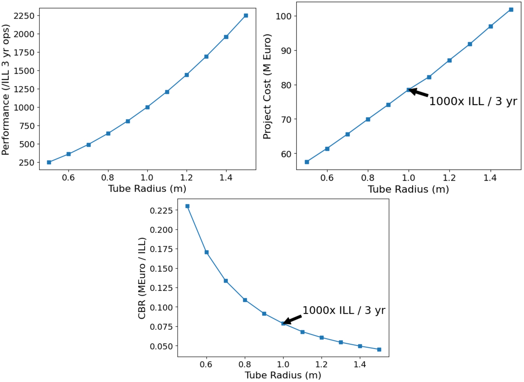
A useful curve to understand the design optimisation is the total instrument cost vs beam radius, r. Whilst the performance of the beam might be expected to increase roughly as a function of beam area, and therefore proportional to
The breakdown of the cost is shown for the baseline
Fig. 90.
Left: breakdown of costs for different parts of the experiment for the baseline selection. Right: breakdown of costs for different parts of the experiment as a function of beam radius.
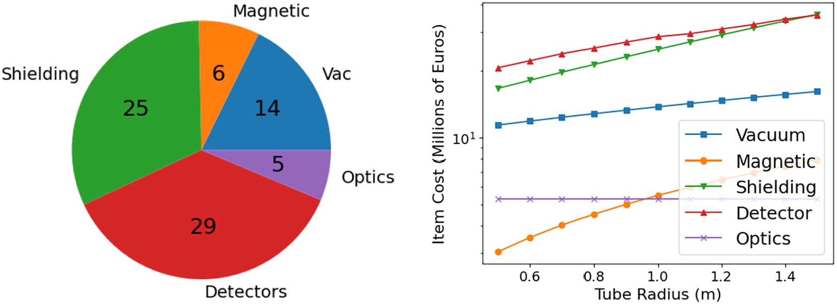
A tabulated breakdown of all the costs for the baseline specifications, length = 200 m,
The cost breakdown given assumes a baseline design with both the vacuum tube and carbon film target having 1 m radius. If the vacuum tube radius is increased by 10 cm to avoid target interactions close to the vacuum tube wall, the overall detector cost would be expected to increase by approximately 4 percent.
From the cost breakdown in Table 13, it can be seen that the lead glass calorimeter (LEC) accounts for the majority of the detector cost. The LEC has a channel count of more than 32000, which is comparable to calorimeters at LHC experiments, and the majority of the cost per LEC counter is the for the silicon photomultipliers (SiPM) used to read out the channels. SiPMs are a relatively economical solution compared to photomultiplier tubes for light detection with high quantum efficiency, and they would be an essential component of any electromagnetic calorimeter design for NNBAR.
The next largest cost comes from the lead-glass blocks. From our experience with the LEC prototype, the glass cost itself represents about 40 percent of this. The type of glass used is mass-produced for applications such as X-ray shielding windows, and the cost per kg assumes raw glass ingots like those purchased for the prototype blocks. The remaining 60 percent of the cost is processing, and based on our cooperation with the Cerfav R&D center in Saint-Gobain for cutting and polishing the glass blocks. Some efficiencies of scale may be possible for the full-scale detector production.
Similarly, the costing for the scintillating stave HRD and veto detectors are based on experience with the HRD prototype, which uses staves from the same Fermilab production facility as those produced for the Mu2e [51] and LDMX [22] experiments.
The TPC prototype developed at LUND is based on the same SAMPA ASICs and similar front-end readout architecture as the ALICE high-luminosity upgrade, and provides the basis for the costing model of that subdetector.
Cost for magnetic shielding is mainly comprised of the material costs of the passive shielding material of about 60 t of sheet material, currently costing 3.7 M Euros annealed; structures amounting to about 1.3 M Euros and 0.5 M Euros for engineering of one section and the adaptation for extreme length. However, with the recent proof of scalability of long octagonal shields in length, the design costs are a fixed offset only.
19.Future steps
The work for conceptual design report identified a range of possible new directions. These are summarised here.
19.1.The NNBAR beamline
This report has identified a number of engineering issues related to how the NNBAR beamline fits into the existing and planned ESS infrastructure.
Preliminary simulations of the shielding thickness of the beamline have been investigated in this report. These indicate that modifications must be made to the ESS bunker. The bunker will need to be reinforced from a shielding perspective. The bunker roof above the NNBAR beamline should be rebuilt.
A shutter system will be needed such that access to the NNBAR detector is enabled without interrupting the ESS operation. The shutter would be designed and integrated in the NNBAR beamline.
Further examination of the current instrument gallery construction inside the D03 building and the connection between its capacity and the capacity of the building’s slab regarding the loads from the shielding and beamline is necessary. An investigation into the possibility of rearranging the installations within the instrument gallery and consideration of groundwater levels, which can impact the extent to which the instrument gallery can be lowered, are necessary.
19.2.Data analysis
The studies performed on data selections used a subset of the observables that will be available. A dedicated vertex finder will be developed and used in future selections. Furthermore, ML showed great promise in rejecting background. A wider range of ML tools will therefore be tested.
19.3.Charged particle tracking
As discussed in Section 14.7, a major future focus will be on the design of the beamline around the detector which dictates the low energy particle flux in the detector. This will also determine the detector granularity. While low energy background will not mimic a signal, it can degrade the ability of the detector to reconstruct signal and distinguish it from background events.
Related to this is a focus on dealing with the constraints of the vacuum vessel and, in particular, the deployment of a tracking system inside the vacuum. Accurate estimates of the low energy particle flux and associated dosages are needed. This work must therefore be performed in tandem with beamline optimization.
Being a large surface, the wall of the vacuum vessel has to be strong to withstand the air pressure outside. A cylindrical shape is thus preferred. In the simulations a homogeneous 2 cm Al tube has been used as it has proven to be strong enough in other applications. The thickness is however critical from the detection point of view. Multiple scattering in the wall will cause angular deviations in so that directions measured outside will not correspond fully to the real directions inside and thus the pointing to the vertex will not be as accurate as it could be. Another obstacle is that a large fraction of the proton spectrum will stop in the wall and will thus not contribute to the vertex definition.
To overcome these problems, a possibility is to place detectors inside the vacuum. The angular deviation by multiple scattering is not large so with good pattern recognition pointing inwards from outside, two high resolution coordinates inside can be sufficient to restore the original direction. Protons stopping in the wall would however not be adequately measured with only two coordinates. A proton track with two coordinates could however still support a hypothetical vertex defined by at least two other tracks. To deal fully with tracks stopping in the wall would require three coordinates. An inner detector system will have the layers to be placed at radial positions of 1–1.5 m depending on position resolution. This amounts to an areal size in excess of around 30 m2 per layer. An absorber layer composed of 6LiF with some backing will likely have to be deployed in front of an inner detector to prevent slow neutrons to enter the tracking. This would also stop the large number of electrons coming from beta decay of free neutrons flying by. This would also serve as a radiation shield radiation shield against cold neutrons. However, inner detectors (and to some extent also outer) can not be shielded from the prompt flux of faster neutrons. Dosages for outer detectors are discussed in Section 15.3.
The obvious choice for detectors in the vacuum would be Si-strip detectors. Since space points are needed it needs crossed strips for each coordinate station. Most pions are minimum ionizing so the noise level is important. A position resolution in the ∼0.1 mm range appears to be adequate if coordinates are around 20 cm apart. The cost of a system with 2 layers (ca 60 m2) would most likely, however, be financially prohibitive. Three layers to manage the lower energy protons even more difficult.
If an inner tracker made of Si Strip detectors could be sufficient for safe tracking one could save money on the outside by omitting the 70 cm taken up by the TPC. That could mean substantial savings on the calorimetry. However a Si-only tracker would most likely need at least 4 stations since normal tracking also uses a known vertex which we don’t have here. The rate of background tracks is of course essential. A helpful property of Si detectors is a quite good time resolution which helps pattern recognition. Another positive aspect is that it performs well not only for perpendicular tracks because of the tiny thickness.
As an alternative to Si, with gas as the detector medium, radiation effects are negligible. Since the particles to track, the pions, are normally minimum ionizing, a gas medium cannot be at low pressure, otherwise efficiency will be lost. Around 50% of normal air pressure would still probably be OK for tracking while energy loss resolution is worsened. Gas detectors placed inside the vacuum must, in addition to being extremely gas tight, also have walls strong enough to withstand the pressure difference to the vacuum. The only possible solution to this would be straw tubes where the cylindrical containment of the gas offers the mechanically strongest barrier. The big obstacle with straws is that they are only position sensitive in 1 dimension (plus the straw radial location). For space points stereo layers of straws will be required, adding to the problem of combinatorial ambiguities. If pattern recognition is provided from outside this may be overcome. The possibility to use the low energy part of the proton spectrum is likely to be diminished or lost if the track is not recognized on the outside.
Construction of straws is a challenge. To cover 5 m at 1 m radius is a bigger project than the ATLAS straw tube project [137]. Probably, for gas tightness one would have to use metallic tubing. One simplification is to use larger tube diameter. That will on the other hand be at the expense of the search window in time to compose coordinates and tracks increases. With 4 mm tubes as in ATLAS the window is 75 ns. This would add to the combinatorial concerns. The diameter of the big vacuum tube will also increase since tubes have to be straight. The feasibility of this type of solution depends a lot on the background conditions. The low energy electron background will make long tracks. The cosmic ray showers, which are the most problematic possible source of fake annihilation signals, have several nearby tracks and will be ambiguous to reconstruct by crossed straws alone. External pattern recognition should help.
An additional alternative is a scintillating fibre tracker. The upgraded forward scintillating fiber tracker of LHCb is a very elegant tracking solution [2]. It requires U,V stereo geometry to obtain space coordinates. Because if its very small readout cell (0.25 mm) one obtains 0.07 mm position resolution perpendicular to the fibre direction. The granularity is very good and the time resolution when assembling coordinates and tracks is on a ns scale. Thus combinatoric ambiguities should be much better in control compared to the straw tubes. Since fibers can adapt (bent) to the cylindrical shape of the tube, the tube diameter does not have to be increased to house the stereo fibers. In size, a 3 station straw tracker for NNBAR would be comparable to the LHCb straw tracker (which has straight fibers) [28]. Outgassing from fibers in vacuum and the sensitivity to radiation are questions that need careful study.
The simulated tube of 2 cm Al is a motivated baseline choice for a conventional beam pipe to maintain a vacuum. However, as discussed, it has negative consequences for the experiment. As an alternative to placing detectors inside the tube, which adds a lot of complication to the setup, a possibility is to spread the 2 cm material in two 1 cm cylinders with spacers between. The strength could be maintained. The inner tracking station as above, could be placed between the cylinders at normal pressure. The material where multiple scattering would stop many protons would be halved. A more advanced solution could be to have a pressure gradient at e.g. 50% of the ambient air pressure in the intermediate volume between the cylinders. Then both cylinder materials could be reduced. One could even place a gaseous tracker operating at 50% of air pressure in the intermediate volume. This volume in itself could be the gas container of that detector. This would be quite elegant if it could be safely implemented; the risk lies is pressure failure (up or down) In the middle volume.
It is also possible to provide the mechanical strength to the cylinder allowing non-uniform thickness and include a skeleton of stronger supports. At first sight this may appear non-optimal, but with external tracking in 3D pointing back to the cylinder, it will be known if a track has passed the thicker material. Such tracks from the analysis can be omitted or weighted down when analysing data.
A further means of mitigating the effect of low energy particles in the tracker is to deploy a magnetic field of up to 0.1 T. This would curl up the Compton electrons. However, it is a notable technical challenge, given the nT-level requirement along the beam path. A possible realization is a toroidal coil in the detector directly at the end of the magnetically shielded vacuum tube. The magnetic shield will then require modifications to separate the flux close to the imperfect toroidal coil and the low-field region,
19.4.Utilizing the ESS pulse shape for neutron focusing
A speculative possibility that can be explored in optics simulations, particularly with the mono-planar nested reflector geometry is to compensate for the gravity effect. Gravitation effectively cuts off the slowest neutrons that contribute most strongly to the
20.Conclusion
The European Spallation Source will open up a new discovery window for searches for baryon number violation. A discovery of free neutron conversions would falsify the Standard Model and address a number of open questions in modern physics including baryogenesis.
This volume outlines a conceptual design of the NNBAR experiment using a dedicated cold moderator. In the HighNESS proposal and in the NNBAR Expression of Interest [69] and white paper [15], it was suggested that NNBAR could achieve a sensitivity that is potentially three orders of magnitude greater than previously achieved [44] with the ESS operating at 5 MW power. This estimate was based on a very preliminary study that did not take into account the ESS design and engineering constraints, which typically tend to reduce sensitivity. However, thanks to the studies made as part of the HighNESS project, including the design of a high performance cold source, nested mirror optics, and annihilation detector, it can be shown in a more realistic way that the proposed sensitivity can be achieved at 2 MW accelerator power. At 5 MW power, the expected sensitivity is more than doubled.
This work has also identified areas for future study. These include further studies on low energy background levels and the exploitation of the prototypes under development. The HIBEAM program, which acts a pilot experiment for NNBAR, will be important. Additional engineering studies are required to ensure that the NNBAR beamline does not interfere with neighbouring beamlines or other ESS facilities.
Notes
1 The first phenomenological model, made within a unification paradigm, was introduced by Mohapatra and Marshak in 1980 [140].
2 Interesting work is ongoing investigating whether materials can be deployed along the guide wall such that the relative phase shifts of the neutron and antineutron wave functions can be small upon reflection [110,144,150]. This has the potential to allow the reduction of the size of a future
5 An identified charged pion pointing to the foil and an identified
6 A dedicated MCNP simulation was used to investigate radiation dosages in the electronics, as described in Section 15.3.
7 The related issue of radiation dosages is discussed in Section 15.3.
8 6Li is likely the optimal neutron poison for NNBAR. Unlike other absorbers such as Cd or B, 6Li has both a large absorption cross section (∼940 b) for thermal neutrons and a dominant absorption reaction (
References
[1] | G. Aad et al., Combined measurement of the Higgs boson mass in |
[2] | R. Aaij et al., The LHCb Upgrade I, Vol. 5: , (2023) . |
[3] | K. Abe et al., Letter of Intent: The Hyper-Kamiokande Experiment – Detector Design and Physics Potential, Vol. 9: , (2011) . |
[4] | K. Abe et al., The search for |
[5] | K. Abe et al., Hyper-Kamiokande design report, 5, (2018) . |
[6] | K. Abe et al., Neutron–antineutron oscillation search using a 0.37 megaton · year exposure of Super-Kamiokande, Phys. Rev. D 103: ((2021) ), 012008. doi:10.1103/PhysRevD.103.012008. |
[7] | S. Abe et al., Search for the Majorana nature of neutrinos in the inverted mass ordering region with KamLAND-Zen, Phys. Rev. Lett. 130: (5) ((2023) ), 051801. doi:10.1103/PhysRevLett.130.051801. |
[8] | C. Abel et al., Measurement of the permanent electric dipole moment of the neutron, Phys. Rev. Lett. 124: (8) ((2020) ), 081803. doi:10.1103/PhysRevLett.124.081803. |
[9] | H. Abele et al., Particle physics at the European Spallation Source, Phys. Rept. 1023: ((2023) ), 1–84. |
[10] | B.B. Abelev et al., Performance of the ALICE experiment at the CERN LHC, Int. J. Mod. Phys. A 29: ((2014) ), 1430044. doi:10.1142/S0217751X14300440. |
[11] | B. Abi et al., Deep Underground Neutrino Experiment (DUNE), far detector technical design report, volume IV: Far detector single-phase technology, JINST 15: (08) ((2020) ), T08010. doi:10.1088/1748-0221/15/08/T08010. |
[12] | B. Abi et al., Deep Underground Neutrino Experiment (DUNE), far detector technical design report, volume II, DUNE Physics. 2: ((2020) ). |
[13] | P. Abratenko et al., First demonstration for a LArTPC-based search for intranuclear neutron–antineutron transitions and annihilation in 40Ar using the, MicroBooNE detector, 8, (2023) . |
[14] | A. Abusleme et al., JUNO physics and detector. Prog. Part. Nucl. Phys. 123: ((2022) ), 103927. doi:10.1016/j.ppnp.2021.103927. |
[15] | A. Addazi et al., New high-sensitivity searches for neutrons converting into antineutrons and/or sterile neutrons at the hibeam/nnbar experiment at the European Spallation Source, Journal of Physics G: Nuclear and Particle Physics 48: (7) ((2021) ), 070501. doi:10.1088/1361-6471/abf429. |
[16] | E.G. Adelberger, C.W. Stubbs, B.R. Heckel, Y. Su, H.E. Swanson, G. Smith, J.H. Gundlach and W.F. Rogers, Testing the equivalence principle in the field of the Earth: Particle physics at masses below 1-microEV?, Phys. Rev. D 42: ((1990) ), 3267–3292. doi:10.1103/PhysRevD.42.3267. |
[17] | J. Adolfsson et al., The upgrade of the ALICE TPC with GEMs and continuous readout, JINST 16: (03) ((2021) ), P03022. doi:10.1088/1748-0221/16/03/P03022. |
[18] | N. Aghanim et al., Planck 2018 results. VI. Cosmological parameters, Astron. Astrophys. 641: ((2020) ), A6, [Erratum: Astron. Astrophys. 652, C4 (2021)]. doi:10.1051/0004-6361/201833910e. |
[19] | L.E. Agnew, T. Elioff, W.B. Fowler, R.L. Lander, W.M. Powell, E. Segrè, H.M. Steiner, H.S. White, C. Wiegand and T. Ypsilantis, Antiproton interactions in hydrogen and carbon below 200 mev, Phys. Rev. 118: ((1960) ), 1371–1391. doi:10.1103/PhysRev.118.1371. |
[20] | S. Agostinelli et al., GEANT4–a simulation toolkit, Nucl. Instrum. Meth. A 506: ((2003) ), 250–303. doi:10.1016/S0168-9002(03)01368-8. |
[21] | B. Aharmim et al., Search for neutron–antineutron oscillations at the Sudbury Neutrino Observatory, Phys. Rev. D 96: (9) ((2017) ), 092005. doi:10.1103/PhysRevD.96.092005. |
[22] | T. Åkesson et al., Light Dark Matter eXperiment (LDMX), 8, (2018) . |
[23] | W.M. Alberico, J. Bernabeu, A. Bottino and A. Molinari, Neutron–antineutron mixing inside nuclei, Nucl. Phys. A 429: ((1984) ), 445–461. doi:10.1016/0375-9474(84)90691-2. |
[24] | W.M. Alberico, A. Bottino and A. Molinari, A new evaluation of the neutron–antineutron oscillation time, Phys. Lett. B 114: ((1982) ), 266–270. doi:10.1016/0370-2693(82)90493-2. |
[25] | W.M. Alberico, A. De Pace and M. Pignone, Neutron – antineutron oscillations in nuclei, Nucl. Phys. A 523: ((1991) ), 488–498. doi:10.1016/0375-9474(91)90032-2. |
[26] | R. Allahverdi, P.S.B. Dev and B. Dutta, A simple testable model of baryon number violation: Baryogenesis, dark matter, neutron–antineutron oscillation and collider signals, Phys. Lett. B 779: ((2018) ), 262–268. doi:10.1016/j.physletb.2018.02.019. |
[27] | I. Altarev, P. Fierlinger, T. Lins, M.G. Marino, B. Nießen, G. Petzoldt, M. Reisner, S. Stuiber, M. Sturm, J. Taggart Singh et al., Minimizing magnetic fields for precision experiments, Journal of Applied Physics 117: (23) ((2015) ), 233903. doi:10.1063/1.4922671. |
[28] | A. Alves Jr. et al., The LHCb detector at the LHC, JINST 3: ((2008) ), S08005. |
[29] | V. Andreev et al., Improved limit on the electric dipole moment of the electron, Nature 562: (7727) ((2018) ), 355–360. doi:10.1038/s41586-018-0599-8. |
[30] | S. Ansell, CombLayer – A fast parametric MCNP(X) model constructor, JAEA-Conf-2015-002, (2016) . |
[31] | L. Aphecetche et al., PHENIX calorimeter, Nucl. Instrum. Meth. A 499: ((2003) ), 521–536. doi:10.1016/S0168-9002(02)01954-X. |
[32] | J.M. Arnold, B. Fornal and M.B. Wise, Simplified models with baryon number violation but no proton decay, Phys. Rev. D 87: ((2013) ), 075004. doi:10.1103/PhysRevD.87.075004. |
[33] | P.B. Arnold and L.D. McLerran, Sphalerons, small fluctuations and baryon bumber violation in electroweak theory, Phys. Rev. D 36: ((1987) ), 581. doi:10.1103/PhysRevD.36.581. |
[34] | I.J. Arnquist et al., Final result of the Majorana demonstrator’s search for neutrinoless double-β decay in Ge76, Phys. Rev. Lett. 130: (6) ((2023) ), 062501. doi:10.1103/PhysRevLett.130.062501. |
[35] | M.T. Arun, Baryon number violation from confining new physics, Phys. Rev. D 107: (5) ((2023) ), 055021. doi:10.1103/PhysRevD.107.055021. |
[36] | K.S. Babu, P.S. Bhupal Dev, E.C.F.S. Fortes and R.N. Mohapatra, Post-sphaleron baryogenesis and an upper limit on the neutron–antineutron oscillation time, Phys. Rev. D 87: (11) ((2013) ), 115019. doi:10.1103/PhysRevD.87.115019. |
[37] | K.S. Babu, P.S.B. Dev and R.N. Mohapatra, Neutrino mass hierarchy, neutron–antineutron oscillation from baryogenesis, Phys. Rev. D 79: ((2009) ), 015017. doi:10.1103/PhysRevD.79.015017. |
[38] | K.S. Babu, R.N. Mohapatra and S. Nasri, Post-sphaleron baryogenesis, Phys. Rev. Lett. 97: ((2006) ), 131301. doi:10.1103/PhysRevLett.97.131301. |
[39] | F. Backman, J. Barrow, Y. Beßler, A. Bianchi, C. Bohm, G. Brooijmans, H. Calen, J. Cederkäll, J.I.M. Damian, E. Dian, D.D. Di Julio, K. Dunne, L. Eklund, M.J. Ferreira, P. Fierlinger, U. Friman-Gayer, C. Happe, M. Holl, T. Johansson, Y. Kamyshkov, E. Klinkby, R. Kolevatov, A. Kupsc, B. Meirose, D. Milstead, A. Nepomuceno, T. Nilsson, A. Oskarsson, H. Perrey, K. Ramic, B. Rataj, N. Rizzi, V. Santoro, S. Silverstein, W.M. Snow, A. Takibayev, R. Wagner, M. Wolke, S.C. Yiu, A.R. Young, L. Zanini and O. Zimmer, The development of the nnbar experiment, Journal of Instrumentation 17: (10) ((2022) ), P10046. doi:10.1088/1748-0221/17/10/P10046. |
[40] | S. Baessler, B.R. Heckel, E.G. Adelberger, J.H. Gundlach, U. Schmidt and H.E. Swanson, Improved test of the equivalence principle for gravitational self-energy, Phys. Rev. Lett. 83: ((1999) ), 3585. doi:10.1103/PhysRevLett.83.3585. |
[41] | M. Bai, V. Shiltsev, G. White and F. Zimmermann, Ultimate limit of future colliders, JACoW NAPAC2022: ((2022) ), 321–324. |
[42] | W. Baldini et al., Measurement of parameters of scintillating bars with wavelength-shifting fibres and silicon photomultiplier readout for the SHiP muon detector, JINST 12: (03) ((2017) ), P03005. doi:10.1088/1748-0221/12/03/P03005. |
[43] | M. Baldo-Ceolin et al., A new experimental limit on neutron-anti neutron transitions, Phys. Lett. B 236: ((1990) ), 95–101. doi:10.1016/0370-2693(90)90601-2. |
[44] | M. Baldo-Ceolin et al., A new experimental limit on neutron – anti-neutron oscillations, Z. Phys. C 63: ((1994) ), 409–416. doi:10.1007/BF01580321. |
[45] | R. Barbier et al., R-parity violating supersymmetry, Phys. Rept. 420: ((2005) ), 1–202. doi:10.1016/j.physrep.2005.08.006. |
[46] | R. Barbieri and A. Masiero, Supersymmetric models with low-energy baryon number violation, Nucl. Phys. B 267: ((1986) ), 679–689. doi:10.1016/0550-3213(86)90136-7. |
[47] | J. Barrow et al., Computing and detector simulation framework for the HIBEAM/NNBAR experimental program at the ESS, EPJ Web Conf. 251: ((2021) ), 02062. doi:10.1051/epjconf/202125102062. |
[48] | J.L. Barrow, Towards neutron transformation searches, PhD thesis, U. Tennessee, Knoxville, (2021) . |
[49] | J.L. Barrow et al., Theories and experiments for testable baryogenesis mechanisms: A snowmass white paper, 3, (2022) . |
[50] | J.L. Barrow, E.S. Golubeva, E. Paryev and J.-M. Richard, Progress and simulations for intranuclear neutron–antineutron transformations in |
[51] | L. Bartoszek et al., Mu2e technical design report, 10, (2014) . |
[52] | G. Battistoni et al., Nucleon stability, magnetic monopoles and atmospheric neutrinos in the Mont Blanc experiment, Phys. Lett. B 133: ((1983) ), 454–460. doi:10.1016/0370-2693(83)90827-4. |
[53] | P. Bentley, Simulated fast neutron instrument backgrounds at a MW Spallation Source, 9, (2022) . |
[54] | P.M. Bentley, Instrument suite cost optimisation in a science megaproject, Journal of Physics Communications 4: ((2020) ), 045014. doi:10.1088/2399-6528/ab8a06. |
[55] | Z. Berezhiani, Mirror world and its cosmological consequences, Int. J. Mod. Phys. A 19: ((2004) ), 3775–3806. doi:10.1142/S0217751X04020075. |
[56] | Z. Berezhiani, More about neutron – mirror neutron oscillation, Eur. Phys. J. C 64: ((2009) ), 421–431. doi:10.1140/epjc/s10052-009-1165-1. |
[57] | Z. Berezhiani, Neutron–antineutron oscillation and baryonic majoron: Low scale spontaneous baryon violation, Eur. Phys. J. C 76: (12) ((2016) ), 705. doi:10.1140/epjc/s10052-016-4564-0. |
[58] | Z. Berezhiani, A possible shortcut for neutron–antineutron oscillation through mirror world, Eur. Phys. J. C 81: (1) ((2021) ), 33. doi:10.1140/epjc/s10052-020-08824-9. |
[59] | Z. Berezhiani and L. Bento, Neutron – mirror neutron oscillations: How fast might they be?, Phys. Rev. Lett. 96: ((2006) ), 081801. doi:10.1103/PhysRevLett.96.081801. |
[60] | Z. Berezhiani, M. Frost, Y. Kamyshkov, B. Rybolt and L. Varriano, Neutron disappearance and regeneration from mirror state, Phys. Rev. D 96: (3) ((2017) ), 035039. doi:10.1103/PhysRevD.96.035039. |
[61] | Z. Berezhiani and A. Vainshtein, Neutron–antineutron oscillation as a signal of CP violation, (2015) . |
[62] | Z. Berezhiani and A. Vainshtein, Neutron–antineutron oscillation and discrete symmetries, Int. J. Mod. Phys. A 33: (31) ((2018) ), 1844016. doi:10.1142/S0217751X18440165. |
[63] | C. Berger et al., Search for neutron–antineutron oscillations in the Frejus detector, Phys. Lett. B 240: ((1990) ), 237–242. doi:10.1016/0370-2693(90)90441-8. |
[64] | J.M. Berryman, S. Gardner and M. Zakeri, Neutron stars with baryon number violation, probing dark sectors, Symmetry 14: (3) ((2022) ), 518. doi:10.3390/sym14030518. |
[65] | T. Bitter and D. Dubbers, Test of the quasifree condition in neutron oscillation experiments, Nuclear Instruments and Methods in Physics Research Section A: Accelerators, Spectrometers, Detectors and Associated Equipment 239: (3) ((1985) ), 461–466. doi:10.1016/0168-9002(85)90024-5. |
[66] | L. Breiman, Random forests, Machine Learning 45: ((2001) ), 5–32, 10. |
[67] | G. Bressi et al., Search for free neutron antineutron oscillations, Z. Phys. C 43: ((1989) ), 175–179. doi:10.1007/BF01588203. |
[68] | G. Bressi et al., Final results of a search for free neutron antineutron oscillations, Nuovo Cim. A 103: ((1990) ), 731–750. doi:10.1007/BF02789025. |
[69] | G. Brooijmans et al., Expression of interest for a new search for neutron–antineutron oscillations at the ESS, (2015) . |
[70] | W. Buchmuller, R.D. Peccei and T. Yanagida, Leptogenesis as the origin of matter, Ann. Rev. Nucl. Part. Sci. 55: ((2005) ), 311–355. doi:10.1146/annurev.nucl.55.090704.151558. |
[71] | M.I. Buchoff and M. Wagman, Neutron–antineutron operator renormalization, PoS LATTICE2014: ((2015) ), 290. |
[72] | M.I. Buchoff and M. Wagman, Perturbative renormalization of neutron–antineutron operators, Phys. Rev. D 93: (1) ((2016) ), 016005, [Erratum: Phys. Rev. D 98, 079901 (2018)]. doi:10.1103/PhysRevD.98.079901. |
[73] | L. Calibbi, G. Ferretti, D. Milstead, C. Petersson and R. Pöttgen, Baryon number violation in supersymmetry: n-nbar oscillations as a probe beyond the LHC, JHEP 05: ((2016) ), 144, [Erratum: JHEP10, 195 (2017)]. doi:10.1007/JHEP05(2016)144. |
[74] | L. Calibbi, G. Ferretti, D.A. Milstead, C. Petersson and R. Poettgen, Baryon number violation in supersymmetry: Neutron–antineutron oscillations as a probe beyond the LHC, PoS LHCP2016: ((2016) ), 152. |
[75] | W.E. Caswell, J. Milutinovic and G. Senjanovic, Matter-antimatter transition operators: A manual for modeling, Phys. Lett. B 122: ((1983) ), 373–377. doi:10.1016/0370-2693(83)91585-X. |
[76] | D. Chang and W. Keung, New limits on R-parity breakings in supersymmetric standard models, Phys. Lett. B 389: ((1996) ), 294–298. doi:10.1016/S0370-2693(96)01271-3. |
[77] | M.L. Cherry, K. Lande, C.K. Lee, R.I. Steinberg and B.T. Cleveland, Experimental test of baryon conservation: A new limit on neutron antineutron oscillations in oxygen, Phys. Rev. Lett. 50: ((1983) ), 1354–1356. doi:10.1103/PhysRevLett.50.1354. |
[78] | J. Chung et al., Search for neutron antineutron oscillations using multiprong events in Soudan 2, Phys. Rev. D 66: ((2002) ), 032004. doi:10.1103/PhysRevD.66.032004. |
[79] | S.N. Co, Supermirrors for Neutrons, (2021) . |
[80] | A.G. Cohen, D.B. Kaplan and A.E. Nelson, Progress in electroweak baryogenesis, Ann. Rev. Nucl. Part. Sci. 43: ((1993) ), 27–70. doi:10.1146/annurev.ns.43.120193.000331. |
[81] | COMSOL AB, COMSOL multiphysics® v. 6.1, (2022) . |
[82] | COMSOL Multiphysics, Introduction to Comsol Multiphysics®, COMSOL Multiphysics, Vol. 9: , Burlington, MA, (1998) , p. 2018. |
[83] | G. Costa and P. Kabir, Environmental effects on possible |
[84] | E.D. Davis and A.R. Young, Neutron–antineutron oscillations beyond the quasifree limit, Phys. Rev. D 95: (3) ((2017) ), 036004. doi:10.1103/PhysRevD.95.036004. |
[85] | S. Dell’Oro, S. Marcocci, M. Viel and F. Vissani, Neutrinoless double beta decay: 2015 review, Adv. High Energy Phys. 2016: ((2016) ), 2162659. |
[86] | P.S.B. Dev and R.N. Mohapatra, TeV scale model for baryon and lepton number violation and resonant baryogenesis, Phys. Rev. D 92: (1) ((2015) ), 016007. doi:10.1103/PhysRevD.92.016007. |
[87] | D. Di DiJulio, I. Svensson, X.X. Cai, J. Cederkall and P. Bentley, Simulating neutron transport in long beamlines at a spallation neutron source using Geant4, Journal of Neutron Research 22: (2–3) ((2020) ), 183–189. doi:10.3233/JNR-190134. |
[88] | Z. Djurcic et al., JUNO conceptual design report, 8, (2015) . |
[89] | M.J. Dolinski, A.W.P. Poon and W. Rodejohann, Neutrinoless double-beta decay: Status and prospects, Ann. Rev. Nucl. Part. Sci. 69: ((2019) ), 219–251. doi:10.1146/annurev-nucl-101918-023407. |
[90] | C.B. Dover, A. Gal and J.M. Richard, Neutron antineutron oscillations in nuclei, Phys. Rev. D 27: ((1983) ), 1090–1100. doi:10.1103/PhysRevD.27.1090. |
[91] | C.B. Dover, A. Gal and J.M. Richard, Neutron antineutron oscillations in nuclei, Nucl. Instrum. Meth. A 284: ((1989) ), 13. doi:10.1016/0168-9002(89)90239-8. |
[92] | K. Dunne, B. Meirose, D. Milstead, A. Oskarsson, V. Santoro, S. Silverstein and S.-C. Yiu, The HIBEAM/NNBAR calorimeter prototype, J. Phys. Conf. Ser. 2374: (1) ((2022) ), 012014. doi:10.1088/1742-6596/2374/1/012014. |
[93] | G.R. Dvali and G. Gabadadze, Nonconservation of global charges in the brane universe and baryogenesis, Phys. Lett. B 460: ((1999) ), 47–57. doi:10.1016/S0370-2693(99)00766-2. |
[94] | Ess instruments. |
[95] | G. Fidecaro et al., Experimental search for neutron antineutron transitions with free neutrons, Phys. Lett. B 156: ((1985) ), 122–128. doi:10.1016/0370-2693(85)91367-X. |
[96] | A. Fomin, A. Serebrov, M. Chaikovskii, O. Zherebtsov, A. Murashkin and E. Golubeva, Project on searching for neutron–antineutron oscillation at the WWR-M reactor, J. Phys. Conf. Ser. 1390: (1) ((2019) ), 012133. doi:10.1088/1742-6596/1390/1/012133. |
[97] | A.K. Fomin, A.P. Serebrov, O.M. Zherebtsov, E.N. Leonova and M.E. Chaikovskii, Experiment on search for neutron–antineutron oscillations using a projected UCN source at the WWR-M reactor, J. Phys. Conf. Ser. 798: (1) ((2017) ), 012115. doi:10.1088/1742-6596/798/1/012115. |
[98] | E. Friedman and A. Gal, Realistic calculations of nuclear disappearance lifetimes induced by neutron–antineutron oscillations, Phys. Rev. D 78: ((2008) ), 016002. doi:10.1103/PhysRevD.78.016002. |
[99] | J.H. Friedman, Greedy function approximation: A gradient boosting machine, Annals of statistics ((2001) ), 1189–1232. |
[100] | M. Frost, Observation of baryon number violation via cold neutron sources, PhD thesis, University of Tennessee, Knoxville, (2019) . |
[101] | K. Fujikawa and A. Tureanu, Parity of the neutron consistent with neutron–antineutron oscillations, Phys. Rev. D 103: (6) ((2021) ), 065017. doi:10.1103/PhysRevD.103.065017. |
[102] | R. Garoby et al., The European Spallation Source design, Physica Scripta 93: (1) ((2017) ), 014001. doi:10.1088/1402-4896/aa9bff. |
[103] | S. Girmohanta and R. Shrock, Baryon-number-violating nucleon and dinucleon decays in a model with large extra dimensions, Phys. Rev. D 101: (1) ((2020) ), 015017. doi:10.1103/PhysRevD.101.015017. |
[104] | S. Girmohanta and R. Shrock, Nucleon decay and |
[105] | J.L. Goity and M. Sher, Bounds on |
[106] | E.S. Golubeva, J.L. Barrow and C.G. Ladd, Model of |
[107] | E.S. Golubeva and L.A. Kondratyuk, Annihilation of low energy antineutrons on nuclei, Nucl. Phys. B Proc. Suppl. 56: ((1997) ), 103–107. doi:10.1016/S0920-5632(97)00260-0. |
[108] | J. Goorley, M. James et al., Initial MCNP6 release overview, Technical report LA-UR-13-22934, Los Alamos National Laboratory, (2013) . |
[109] | T. Goorley, M. James, T. Booth, F. Brown, J. Bull, L. Cox, J. Durkee, J. Elson, M. Fensin, R. Forster, J. Hendricks, H. Hughes, R. Johns, B. Kiedrowski, R. Martz, S. Mashnik, G. Mckinney, D. Pelowitz, R. Prael and T. Zukaitis, Initial mcnp6 release overview. mcnp6 version 0.1, Nuclear technology 180: ((2012) ), 298–315, 12. |
[110] | V. Gudkov et al., A possible neutron–antineutron oscillation experiment at PF1B at the Institut Laue Langevin, Symmetry 13: (12) ((2021) ), 2314. doi:10.3390/sym13122314. |
[111] | V. Gudkov, V.V. Nesvizhevsky, K.V. Protasov, W.M. Snow and A.Y. Voronin, A new approach to search for free neutron–antineutron oscillations using coherent neutron propagation in gas, Physics Letters B 808: ((2020) ), 135636. doi:10.1016/j.physletb.2020.135636. |
[112] | J. Gustafson et al., Search for dinucleon decay into pions at Super-Kamiokande, Phys. Rev. D 91: (7) ((2015) ), 072009. doi:10.1103/PhysRevD.91.072009. |
[113] | C. Hagmann, D. Lange and D. Wright, Cosmic-ray shower generator (cry) for Monte Carlo transport codes, in: 2007 IEEE Nuclear Science Symposium Conference Record, Vol. 2: , (2007) , pp. 1143–1146. doi:10.1109/NSSMIC.2007.4437209. |
[114] | I. Halm, Neutron–antineutron oscillations and primordial nucleosynthesis, EPL 8: ((1989) ), 703–708. doi:10.1209/0295-5075/8/7/021. |
[115] | Highness, https://highnessproject.eu/. |
[116] | M. Holl, R. Kolevatov, B. Meirose, D. Milstead, B. Rataj, V. Santoro and L. Zanini, Beamline simulation for the nnbar experiment at the European Spallation Source, (2022) . |
[117] | S.J. Huber, M. Pospelov and A. Ritz, Electric dipole moment constraints on minimal electroweak baryogenesis, Phys. Rev. D 75: ((2007) ), 036006. doi:10.1103/PhysRevD.75.036006. |
[118] | J. Hufner and B.Z. Kopeliovich, Neutron – antineutron oscillations in nuclei revisited, Mod. Phys. Lett. A 13: ((1998) ), 2385–2392. doi:10.1142/S0217732398002540. |
[119] | V.K. Ignatovich, On |
[120] | A.J. Izenman, Linear Discriminant Analysis, Springer, New York, New York, NY, (2008) , pp. 237–280. |
[121] | D. Jason Koskinen, (TMVA group), H. Voss and (MPIK), Lecture 10: Multivariate method – boosted decision tree, (2021) . |
[122] | T.W. Jones et al., A search for |
[123] | Y. Kamyshkov et al., Use of Cold Source and Large Reflector Mirror Guide for Neutron–Antineutron Oscillation Search, (1995) , pp. 843–849. |
[124] | Y. Kamyshkov, M. Snow and G. Greene, Time-variable neutron optics (unpublished). |
[125] | M.V. Kazarnovskiǐ, V.A. Kuz’min and M.E. Shaposhnikov, Nbar n oscillations: The possibility of observing them using ultracold neutrons, Soviet Journal of Experimental and Theoretical Physics Letters 34: ((1981) ), 47. |
[126] | B.O. Kerbikov, Lindblad and Bloch equations for conversion of a neutron into an antineutron, Nuclear Physics A 975: ((2018) ), 59–72. doi:10.1016/j.nuclphysa.2018.04.006. |
[127] | B.O. Kerbikov, A.E. Kudryavtsev and V.A. Lensky, Neutron–antineutron oscillations in a trap revisited, Journal of Experimental and Theoretical Physics 98: ((2004) ), 417–426. doi:10.1134/1.1705693. |
[128] | T. Kittelmann, E. Klinkby, E.B. Knudsen, P. Willendrup, X.X. Cai and K. Kanaki, Monte Carlo Particle Lists: MCPL, Computer Physics Communications 218: ((2017) ), 17–42. doi:10.1016/j.cpc.2017.04.012. |
[129] | F.R. Klinkhamer and N.S. Manton, A saddle point solution in the Weinberg–Salam theory, Phys. Rev. D 30: ((1984) ), 2212. doi:10.1103/PhysRevD.30.2212. |
[130] | M.R. Krishnaswamy, M.G.K. Menon, N.K. Mondal, V.S. Narasimham, B.V. Sreekantan, Y. Hayashi, N. Ito, S. Kawakami and S. Miyake, Results from the KGF proton decay experiment, Nuovo Cim. C 9: ((1986) ), 167–181, [Conf. Proc. C850418, 97(1985)] |
[131] | V.A. Kuzmin, CP violation and baryon asymmetry of the universe, Pisma Zh. Eksp. Teor. Fiz. 12: ((1970) ), 335–337. |
[132] | V.A. Kuzmin, V.A. Rubakov and M.E. Shaposhnikov, On the anomalous electroweak baryon number nonconservation in the early universe, Phys. Lett. B 155: ((1985) ), 36. doi:10.1016/0370-2693(85)91028-7. |
[133] | P. Langacker, Grand unified theories and proton decay, Phys. Rept. 72: ((1981) ), 185. doi:10.1016/0370-1573(81)90059-4. |
[134] | M.A. Luty, Baryogenesis via leptogenesis, Phys. Rev. D 45: ((1992) ), 455–465. doi:10.1103/PhysRevD.45.455. |
[135] | R.B. Mann, An Introduction to Particle Physics and the Standard Model, CRC Press, Boca Raton, FL, (2010) . |
[136] | N.S. Manton, Topology in the Weinberg–Salam theory, Phys. Rev. D 28: ((1983) ), 2019. doi:10.1103/PhysRevD.28.2019. |
[137] | B. Mindur, ATLAS transition radiation tracker (TRT): Straw tubes for tracking and particle identification at the Large Hadron Collider, Nucl. Instrum. Meth. A 845: ((2017) ), 257–261. doi:10.1016/j.nima.2016.04.026. |
[138] | R.N. Mohapatra, Neutron-anti-neutron oscillation: Theory and phenomenology, J. Phys. G 36: ((2009) ), 104006. doi:10.1088/0954-3899/36/10/104006. |
[139] | R.N. Mohapatra, From old symmetries to new symmetries: Quarks, leptons and |
[140] | R.N. Mohapatra and R.E. Marshak, Local |
[141] | R.N. Mohapatra and G. Senjanovic, Neutrino masses and mixings in gauge models with spontaneous parity violation, Phys. Rev. D 23: ((1981) ), 165. doi:10.1103/PhysRevD.23.165. |
[142] | R.N. Mohapatra and G. Senjanovic, Spontaneous breaking of global |
[143] | D.E. Morrissey and M.J. Ramsey-Musolf, Electroweak baryogenesis, New J. Phys. 14: ((2012) ), 125003. doi:10.1088/1367-2630/14/12/125003. |
[144] | V.V. Nesvizhevsky, V. Gudkov, K.V. Protasov, W.M. Snow and A.Y. Voronin, Experimental approach to search for free neutron–antineutron oscillations based on coherent neutron and antineutron mirror reflection, Phys. Rev. Lett. 122: (22) ((2019) ), 221802. doi:10.1103/PhysRevLett.122.221802. |
[145] | S. Nussinov and R. Shrock, N – anti-N oscillations in models with large extra dimensions, Phys. Rev. Lett. 88: ((2002) ), 171601. doi:10.1103/PhysRevLett.88.171601. |
[146] | F. Oosterhof, B. Long, J. de Vries, R.G.E. Timmermans and U. van Kolck, Baryon-number violation by two units and the deuteron lifetime, Phys. Rev. Lett. 122: (17) ((2019) ), 172501. doi:10.1103/PhysRevLett.122.172501. |
[147] | S. Peggs, ESS technical design report, (2013) . |
[148] | D.G. Phillips II. et al., Neutron–antineutron oscillations: Theoretical status and experimental prospects, Phys. Rept. 612: ((2016) ), 1–45. doi:10.1016/j.physrep.2015.11.001. |
[149] | D.M.W. Powers, Evaluation: From precision, recall and f-measure to roc, informedness, markedness and correlation, CoRR, (2020) , arXiv:2010.16061. |
[150] | K.V. Protasov, V. Gudkov, E.A. Kupriyanova, V.V. Nesvizhevsky, W.M. Snow and A.Y. Voronin, Theoretical analysis of antineutron-nucleus data needed for antineutron mirrors in neutron–antineutron oscillation experiments, Phys. Rev. D 102: ((2020) ), 075025. doi:10.1103/PhysRevD.102.075025. |
[151] | S. Rao and R. Shrock, |
[152] | S. Rao and R.E. Shrock, Six fermion ( |
[153] | J. Riedlberger et al., Anti-proton annihilation at rest in nitrogen and deuterium gas, Phys. Rev. C 40: ((1989) ), 2717–2731. doi:10.1103/PhysRevC.40.2717. |
[154] | E. Rinaldi, S. Syritsyn, M.L. Wagman, M.I. Buchoff, C. Schroeder and J. Wasem, Neutron–antineutron oscillations from lattice QCD, Phys. Rev. Lett. 122: (16) ((2019) ), 162001. doi:10.1103/PhysRevLett.122.162001. |
[155] | E. Rinaldi, S. Syritsyn, M.L. Wagman, M.I. Buchoff, C. Schroeder and J. Wasem, Lattice QCD determination of neutron–antineutron matrix elements with physical quark masses, Phys. Rev. D 99: (7) ((2019) ), 074510. doi:10.1103/PhysRevD.99.074510. |
[156] | D. Rodriguez, S. Kennedy and P. Bentley, Properties of elliptical guides for neutron beam transport and applications for new instrumentation concepts, 44: (4) ((2011) ), 727–737. |
[157] | D. Rohr, S. Gorbunov, M.O. Schmidt and R. Shahoyan, GPU-based online track reconstruction for the ALICE TPC in run 3 with continuous read-out, EPJ Web Conf. 214: ((2019) ), 01050. doi:10.1051/epjconf/201921401050. |
[158] | T.S. Roussy et al., An improved bound on the electron’s electric dipole moment, Science 381: (6653) ((2023) ), adg4084. |
[159] | A.D. Sakharov, Violation of CP invariance, C asymmetry, and baryon asymmetry of the universe, Pisma Zh. Eksp. Teor. Fiz. 5: ((1967) ), 32–35. |
[160] | V. Santoro, The HighNESS project and future free neutron oscillations searches at the ESS, PoS EPS-HEP2021: ((2022) ), 711. |
[161] | V. Santoro et al., HighNESS conceptual design report volume I, Journal of Neutron Research ((2024) ). |
[162] | V. Santoro, K.H. Andersen, P. Bentley, M. Bernasconi, M. Bertelsen, Y. Beßler, A. Bianchi, T. Brys, D. Campi, A. Chambon, V. Czamler, D.D. Di Julio, E. Dian, K. Dunne, M.J. Ferreira, P. Fierlinger, U. Friman-Gayer, B.T. Folsom, A. Gaye, G. Gorini, C. Happe, M. Holl, Y. Kamyshkov, T. Kittelmann, E.B. Klinkby, R. Kolevatov, S.I. Laporte, B. Lauritzen, J.I. Marquez Damian, B. Meirose, F. Mezei, D. Milstead, G. Muhrer, V. Neshvizhevsky, B. Rataj, N. Rizzi, L. Rosta, S. Samothrakitis, H. Schober, J.R. Selknaes, S. Silverstein, M. Strobl, M. Strothmann, A. Takibayev, R. Wagner, P. Willendrup, S. Xu, S.C. Yiu, L. Zanini and O. Zimmer, The highness project at the European Spallation Source: Current status and future perspectives, Nuclear Science and Engineering 0: (0) ((2023) ), 1–33. |
[163] | V. Santoro, K.H. Andersen, M. Bernasconi, M. Bertelsen, Y. Beßler, D. Campi, V. Czamler, D.D. Di Julio, E. Diane, K. Dunne, P. Fierlinger, A. Gaye, G. Gorini, C. Happe, T. Kittelmann, E.B. Klinkby, Z. Kokai, R. Kolevatov, B. Lauritzen, R. Linander, J.I. Marquez Damian, B. Meirose, F. Mezei, D. Milstead, G. Muhrer, K. Ramic, B. Rataj, N. Rizzi, S. Samothrakitis, J.R. Selknaes, S. Silverstein, M. Strobl, M. Strothmann, A. Takibayev, R. Wagner, P. Willendrup, S.C. Yiu, L. Zanini and O. Zimmer, Development of a high intensity neutron source at the European Spallation Source: The highness project, (2022) . |
[164] | V. Santoro, D.D. Di Julio and P.M. Bentley, MeV neutron production from thermal neutron capture in 6^Li simulated with Geant4, J. Phys. Conf. Ser. 746: (1) ((2016) ), 012012. |
[165] | V. Santoro, D. Milstead, P. Fierlinger, W.M. Snow, J. Barrow, M. Bartis, P. Bentley, L. Bjork, G. Brooijmans, N. de la Cour, D.D. Di Julio, K. Dunne, M.J. Ferreira, U. Friman-Gayer, M. Holl, Y. Kamyshkov, E. Kemp, M. Kickulies, R. Kolevatov, H.T. Johansson, B. Jonsson, W. Lejon, J.I. Marquez Damian, B. Meirose, A. Nepomuceno, T. Nilsson, A. Oskarsson, R. Pasechnik, L. Persson, B. Rataj, S. Silverstein, R. Wagner, M. Wolke, S.C. Yiu and L. Zanini, (2023) , The hibeam program: Search for neutron oscillations at the ess. |
[166] | T. Sato, Y. Iwamoto, S. Hashimoto, T. Ogawa, T. Furuta, S. Ichiro Abe, T. Kai, P.-E. Tsai, N. Matsuda, H. Iwase, N. Shigyo, L. Sihver and K. Niita, Features of particle and heavy ion transport code system (phits) version 3.02, Journal of Nuclear Science and Technology 55: (6) ((2018) ), 684–690. doi:10.1080/00223131.2017.1419890. |
[167] | S. Schlamminger, K.Y. Choi, T.A. Wagner, J.H. Gundlach and E.G. Adelberger, Test of the equivalence principle using a rotating torsion balance, Phys. Rev. Lett. 100: ((2008) ), 041101. doi:10.1103/PhysRevLett.100.041101. |
[168] | U. Schmidt, T. Bitter, P. El-Muzeini, D. Dubbers and O. Scharpf, Long distance propagation of a polarized neutron beam in zero magnetic field, Nuclear Instruments and Methods in Physics Research Section A: Accelerators, Spectrometers, Detectors and Associated Equipment 320: (3) ((1992) ), 569–573. doi:10.1016/0168-9002(92)90952-Z. |
[169] | G. Senjanovic, Spontaneous breakdown of parity in a class of gauge theories, Other thesis, (1979) . |
[170] | G. Senjanovic, Higgs mass scales and matter-antimatter oscillations in grand unified theories, in: Workshop on Neutrino-Antineutrino Oscillations, Vol. 4: , (1982) . |
[171] | G. Senjanovic and R.N. Mohapatra, Exact left-right symmetry and spontaneous violation of parity, Phys. Rev. D 12: ((1975) ), 1502. doi:10.1103/PhysRevD.12.1502. |
[172] | A.P. Serebrov, A.K. Fomin and Y.A. Kamyshkov, Sensitivity of experiment on search for neutron–antineutron oscillations on the projected ultracold neutron source at the wwr-m reactor, Technical Physics Letters 42: ((2016) ), 99–101. doi:10.1134/S1063785016010314. |
[173] | V. Shiltsev and F. Zimmermann, Modern and future colliders, Rev. Mod. Phys. 93: ((2021) ), 015006. doi:10.1103/RevModPhys.93.015006. |
[174] | H.M. Shimizu, Optimization of Supermirror, (2014) . |
[175] | A.M. Sirunyan et al., A measurement of the Higgs boson mass in the diphoton decay channel, Phys. Lett. B 805: ((2020) ), 135425. doi:10.1016/j.physletb.2020.135425. |
[176] | C. Sivaram and V. Krishan, Neutron oscillation as a source of excess sub-GeV antiprotons in galactic cosmic rays, Nature 299: ((1982) ), 427–428. doi:10.1038/299427a0. |
[177] | G.L. Smith, C.D. Hoyle, J.H. Gundlach, E.G. Adelberger, B.R. Heckel and H.E. Swanson, Short range tests of the equivalence principle, Phys. Rev. D 61: ((2000) ), 022001. doi:10.1103/PhysRevD.61.022001. |
[178] | S.A. Stephens and R.L. Golden, The role of antiprotons in cosmic-ray physics, Space science reviews 46: (1–2) ((1988) ), 31–91. doi:10.1007/BF00173875. |
[179] | G.R. Stevenson and R.H. Thomas, A simple procedure for the estimation of neutron skyshine from proton accelerators, Health physics 46: (1) ((1984) ), 115–122. doi:10.1097/00004032-198401000-00009. |
[180] | Y. Su, B.R. Heckel, E.G. Adelberger, J.H. Gundlach, M. Harris, G.L. Smith and H.E. Swanson, New tests of the universality of free fall, Phys. Rev. D 50: ((1994) ), 3614–3636. doi:10.1103/PhysRevD.50.3614. |
[181] | A.H. Sullivan, A Guide to Radiation and Radioactivity Levels Near High Energy Particle Acelerators, Nuclear Technology Publishing. |
[182] | Z. Sun, P. Fierlinger, J. Han, L. Li, T. Liu, A. Schnabel, S. Stuiber and J. Voigt, Limits of low magnetic field environments in magnetic shields, IEEE Transactions on Industrial Electronics 68: (6) ((2020) ), 5385–5395. doi:10.1109/TIE.2020.2987267. |
[183] | Z. Sun, M. Reisner, P. Fierlinger, A. Schnabel, S. Stuiber and L. Li, Dynamic modeling of the behavior of permalloy for magnetic shielding, Journal of Applied Physics 119: (19) ((2016) ), 193902. doi:10.1063/1.4949516. |
[184] | S. Sussman et al., Dinucleon and nucleon decay to two-body final states with no hadrons in Super-Kamiokande, (2018) . |
[185] | G. ’t Hooft, Symmetry breaking through Bell–Jackiw anomalies, Phys. Rev. Lett. 37: ((1976) ), 8–11. doi:10.1103/PhysRevLett.37.8. |
[186] | A. Takenaka et al., Search for proton decay via |
[187] | V. Takhistov et al., Search for nucleon and dinucleon decays with an invisible particle and a charged lepton in the final state at the Super-Kamiokande experiment, Phys. Rev. Lett. 115: (12) ((2015) ), 121803. doi:10.1103/PhysRevLett.115.121803. |
[188] | M. Takita et al., A search for neutron – antineutron oscillation in a 16O nucleus, Phys. Rev. D 34: ((1986) ), 902. doi:10.1103/PhysRevD.34.902. |
[189] | Technical report ESS-0001786, (2015) |
[190] | The ATLAS Collaboration, Measurement of the Higgs boson mass with |
[191] | M. Trodden, Electroweak baryogenesis, Rev. Mod. Phys. 71: ((1999) ), 1463–1500. doi:10.1103/RevModPhys.71.1463. |
[192] | Update of the european strategy for particle, physics, CERN-ESU-015-2020, (2020) . |
[193] | |
[194] | J.D. Vergados, H. Ejiri and F. Simkovic, Theory of neutrinoless double beta decay, Rept. Prog. Phys. 75: ((2012) ), 106301. doi:10.1088/0034-4885/75/10/106301. |
[195] | P. Willendrup, E. Farhi, E. Knudsen, U. Filges and K. Lefmann, Component manual for the neutron ray-tracing package McStas, (2020) , http://www.mcstas.org/documentation/manual/mcstas-2.7-components.pdf. |
[196] | P. Willendrup, E. Farhi and K. Lefmann, Mcstas 1.7 – a new version of the flexible Monte Carlo neutron scattering package, Physica B: Condensed Matter 350: (1, Supplement) ((2004) ), E735–E737. |
[197] | E. Wodey, D. Tell, E.M. Rasel, D. Schlippert, R. Baur, U. Kissling, B. Kölliker, M. Lorenz and M. Marrer, Urs Schläpfer et al. a scalable high-performance magnetic shield for very long baseline atom interferometry, Review of Scientific Instruments 91: (3) ((2020) ), 035117. doi:10.1063/1.5141340. |
[198] | R.L. Workman et al., Review of particle physics, PTEP 2022: ((2022) ), 083C01. |
[199] | S. Yiu et al., Status of the design of an annihilation detector to observe neutron–antineutron conversions at the European Spallation Source, Symmetry 14: (1) ((2022) ), 76. doi:10.3390/sym14010076. |
[200] | L. Zanini, D. DiJulio, S. Kennedy, E. Klinkby and V. Santoro, Neutronic design of the bunker shielding for the ESS, Journal of Surface Investigation: X-ray, Synchrotron and Neutron Techniques 14: (1) ((2020) ), S251–S253. doi:10.1134/S1027451020070538. |
[201] | O. Zimmer, Multi-mirror imaging optics for low-loss transport of divergent neutron beams and tailored wavelength spectra, (2016) , arXiv:1611.07353 [hep-ex, physics:nucl-ex, physics:physics]. |
[202] | O. Zimmer, Imaging nested-mirror assemblies – a new generation of neutron delivery systems?, Journal of Neutron Research 20: (4) ((2019) ), 91–98. doi:10.3233/JNR-190101. |
[203] | F. Zwirner, Observable delta |


