
Systematic underestimation of uncertainties by widespread neutron-scattering data-reduction software
Abstract
Data-reduction software used at neutron-scattering facilities around the world, Mantid and Scipp, ignore correlations when propagating uncertainties in arithmetic operations. Normalization terms applied during data-reduction frequently have a lower dimensionality than the quantities being normalized. We show how the lower dimensionality introduces correlations, which the software does not take into account in subsequent data-reduction steps such as histogramming, summation, or fitting. As a consequence, any uncertainties in the normalization terms are strongly suppressed and thus effectively ignored. This can lead to erroneous attribution of significance to deviations that are actually pure noise, or to overestimation of significance in final data-reduction results that are used for further data analysis. We analyze this flaw for a number of different cases as they occur in practice. For the two concrete experiments that are comprised in these case studies the underestimation turns out to be of negligible size. There is however no reason to assume that this generalizes to other measurements at the same or at different neutron-scattering beamlines. We describe and implement a potential solution that yields not only corrected error estimates but also the full variance-covariance matrix of the reduced result with minor additional computational cost.
1.Introduction
The number of neutron counts measured in a detector element during a neutron-scattering experiment follows a Poisson distribution. In practice this is typically handled with a Gaussian approximation, setting the standard-deviation
One caveat in both Mantid and Scipp is that correlations are not taken into account in the propagation of uncertainties. This is generally not considered a problem since the raw data are assumed to be uncorrelated. However, as we will show, ubiquitous operations in neutron-scattering data-reduction introduce such correlations in intermediate computation steps but subsequently fail to take these into account. This leads to a systematic underestimation of uncertainties in final results such as
The remainder of this work is organized as follows. We describe the problem in Section 2. In Section 3 we analyze a couple of concrete examples, in particular for small-angle neutron scattering (SANS) and powder diffraction. Furthermore, we derive full expressions for the variance-covariance matrices of the reduced data, which turn out to be simple and computationally tractable. We confirm the correctness of the improved estimates for the uncertainties using a bootstrapping [9] approach. The results are discussed in Section 4 and we draw conclusions in Section 5.
2.Problem description
For neutron-scattering data-reduction the most relevant operations that require handling of uncertainties are addition, multiplication, and division. Normalization operations can be implemented as division or as multiplication with the inverse. The Taylor series expansion (truncated after first order) for uncertainty propagation [3] gives
The most straightforward example of the incorrect treatment of correlations is the computation of a histogram of event data after normalization. As described in [19], CS event-mode normalization first histograms the normalization term. Then, for every event of the data to normalize, the corresponding bin in the normalization histogram is identified and the event weight is scaled with the inverse of the value of that bin. We consider a single bin with n events, their weights
Concretely, for the example of histogramming event data, all neutrons typically have the same initial weight
To illustrate this effect, we show in Fig. 1 how the relative uncertainty for a histogram of normalized event data scales with the number of events. Both the CS implementation (×) and the V0 approximation (+) of event-mode normalization lead to a relative error of the histogrammed result that goes to 0 with increasing event count. Importantly, CS and V0 yield near-identical results for all values of C. In contrast, normalization after histogramming (∙) or correct handling of correlations yields a relative error limited by the relative error of the normalization factor.
Fig. 1.
Relative error
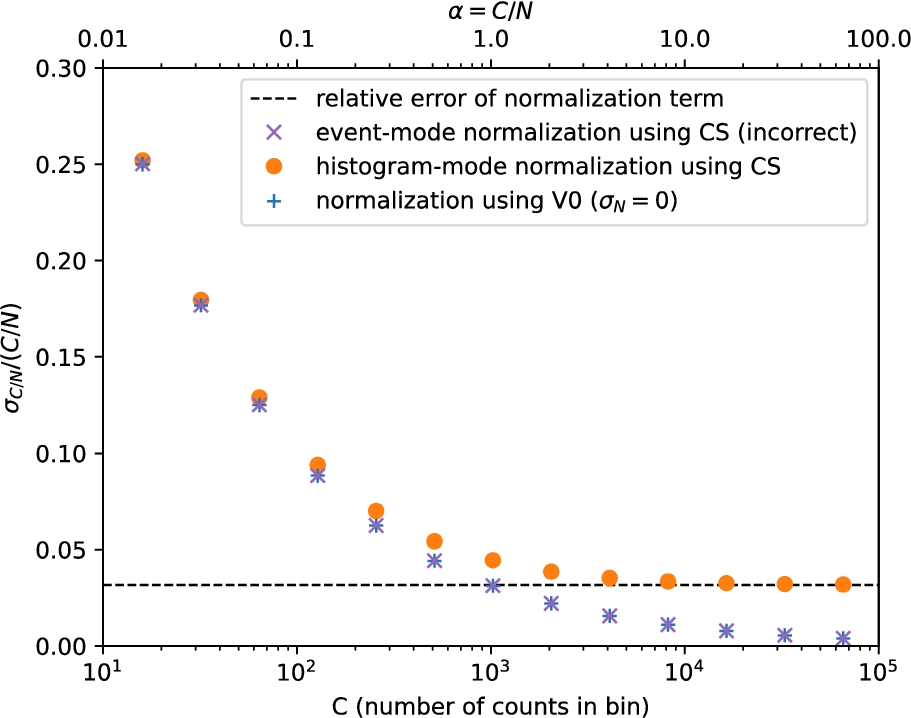
In summary, the CS approach is thus either wasteful (since it is equivalent to V0 with additional compute overhead), or incorrect. In the next section we analyze more complex cases, namely normalization in SANS and powder diffraction workflows. These involve a transformation of coordinates66 after the normalization step but before a histogramming/summing step. While the problem of the CS approach is conceptually the same, the concrete effects are thus slightly harder to visualize and grasp.
3.Case studies
3.1.SANS
In a time-of-flight SANS experiment, the differential scattering cross section
In the SANS case the CS calculation of the normalization term itself (rather than the normalization of the detector counts) in Eq. (17) suffers from the issue described in Section 2. In contrast to the example from Fig. 1, the problem here is not caused by event-mode normalization, but by a different type of broadcast operation. Since the λ-dependent factors in the denominator do not depend on i and j, and the solid angle
Note that there are a number of other contributions to the uncertainties with similar issues, which we ignored in this analysis. Our goal here is to provide an example for illustration of the problems in CS, not a complete analysis of the entire SANS data reduction. See the discussion in Section 4 for more background.
To illustrate the issue we study the data-reduction workflow for an experiment on non-ionic surfactants that was carried out at the Sans2d instrument [22] at the ISIS facility at the STFC Rutherford Appleton Laboratory.99 The SANS reduction workflow we used can be found online at [21]. A key factor in determining whether the CS implementation is adequate is the ratio of total detector counts to total monitor counts1010
Fig. 2.
(a) The scattering differential cross-section
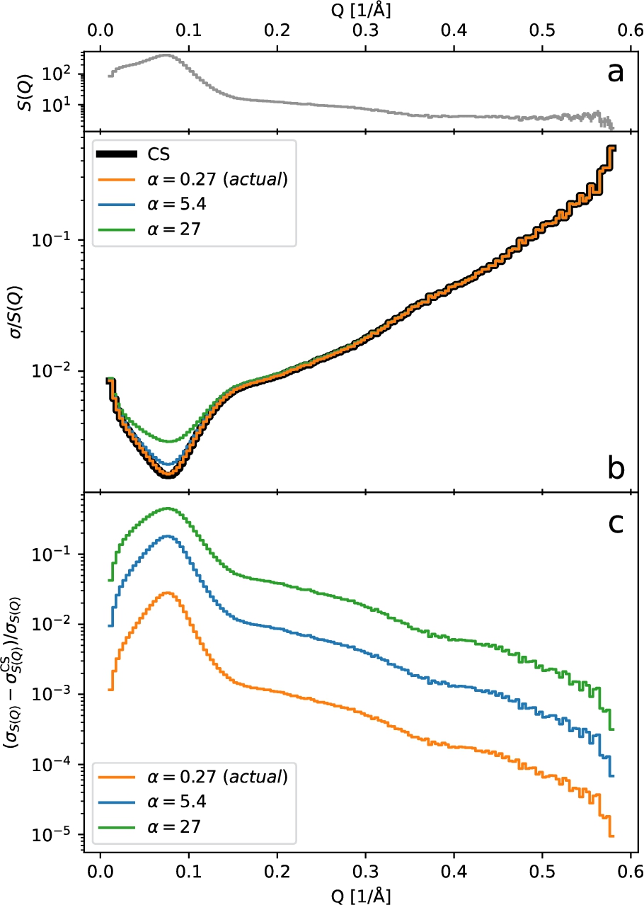
Fig. 3.
Comparison of the relative standard deviation for
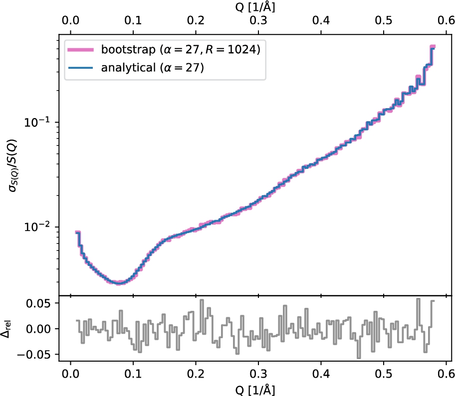
As a verification of these results, we independently computed the uncertainties by using a bootstrap [9] method – a sampling technique that can be used to estimate the distribution of a statistic.1111 It involves repeatedly sampling from a population with replacement, and then calculating the statistic of interest for each sample. The resulting distribution of statistics can then be used to calculate a confidence interval for the population parameter. This approach is useful because it allows us to make inferences about a population even when we do not have a theoretical distribution for the statistic of interest. The biggest advantage of this approach is its simplicity, but it comes at a high cost – in our case we need to repeat the entire data-reduction for every bootstrap sample, i.e., hundreds or thousands of times. The bootstrapping approach is described in some more detail in Appendix A. We can see in Fig. 3 that there is an excellent agreement between the bootstrap results and our analytical derivation (see Appendix A, in particular Fig. 8 which shows the same result for
The correct (first order) expression for the uncertainties for this reduction workflow can be derived in a straightforward manner. We adopt a simpler and more generic notation equivalent to Eq. (17) as follows. We define
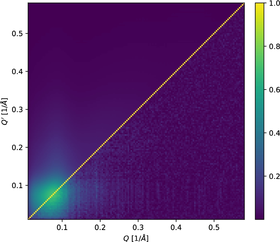
The diagonal component of this result is included in Fig. 2. In addition, we show the resulting Pearson correlation matrix
Fig. 4.
Correlation matrices for the time-of-flight SANS-reduction workflow using
3.2.Powder diffraction
We consider a simplified model of a time-of-flight powder-diffraction reduction workflow based on the workflow used at ISIS [15]. Our model workflow consists of the following steps: (1) compute wavelength coordinates for detector data and monitor data, (2) compute wavelength histograms, (3) normalize the detector data by the monitor, (4) compute d-spacing coordinate for detector data, and (5) compute d-spacing histogram, combining data from all (or a user-defined subset of) detector pixels. This yields the normalized d-spacing spectrum
In Fig. 5 we compare the uncertainties computed by CS and by an improved analytical approach which will be described below. Source code for reproducing these results can be found in the supplementary material [13]. As described in Section 3.1, we study the influence of the ratio of total detector to monitor counts, α (defined equivalently to Eq. (19)), influenced, e.g., by the sample volume. For
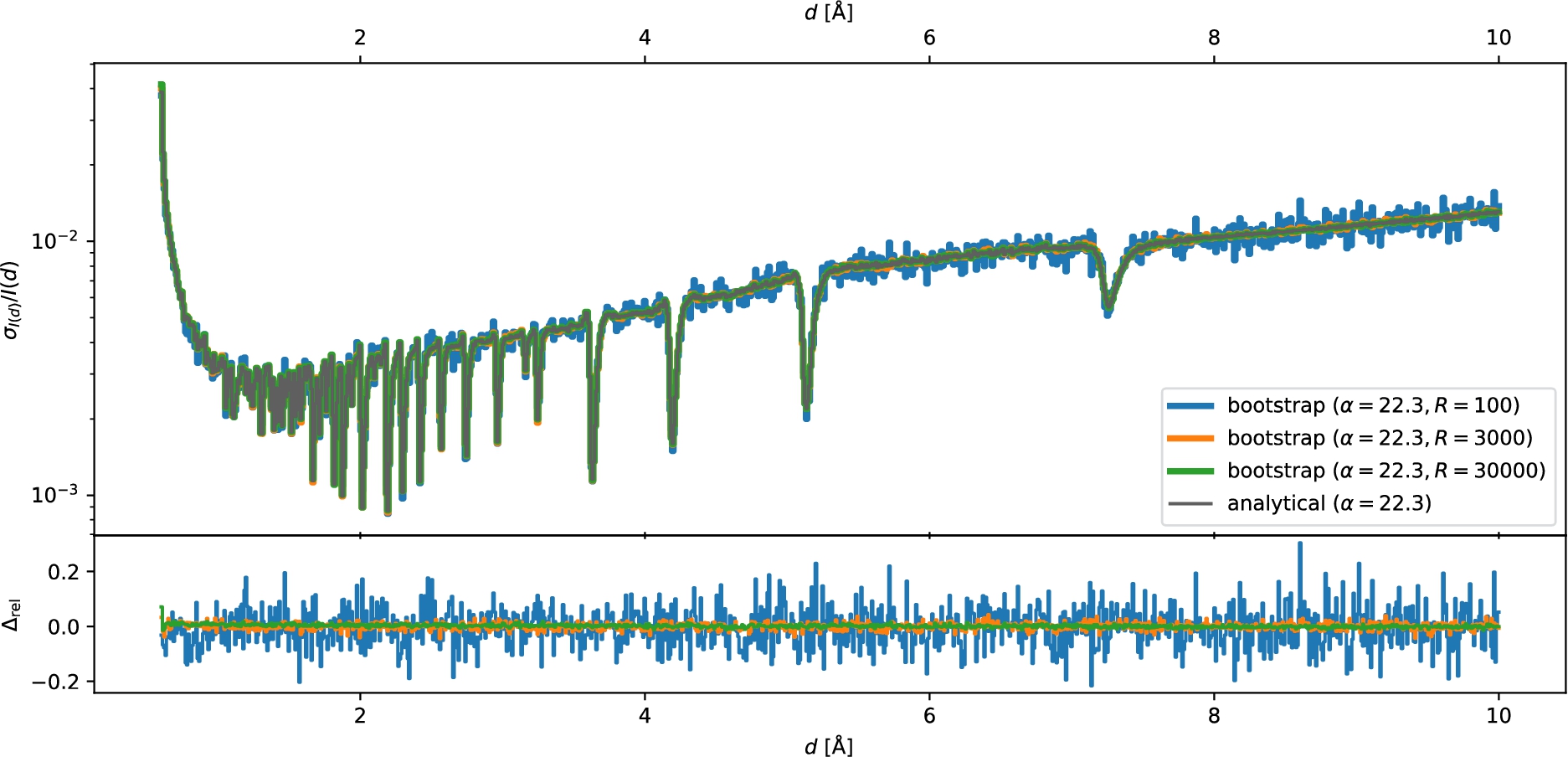
Fig. 5.
Top:
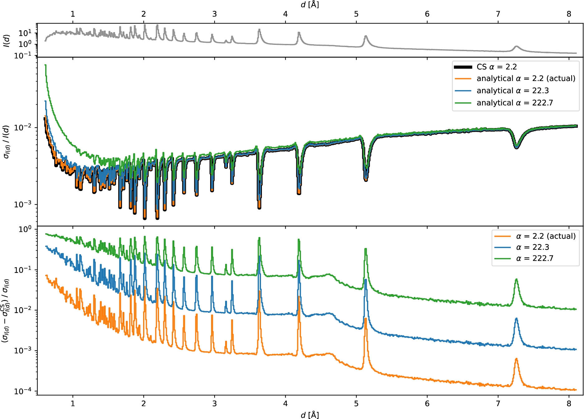
Fig. 6.
Comparison of the relative standard deviation for
For the simplified model workflow we can derive the correct (first order) expression for the uncertainties in a straightforward manner. This also provides the covariances or correlations between different d-spacing values. We adopt the following notation. Let
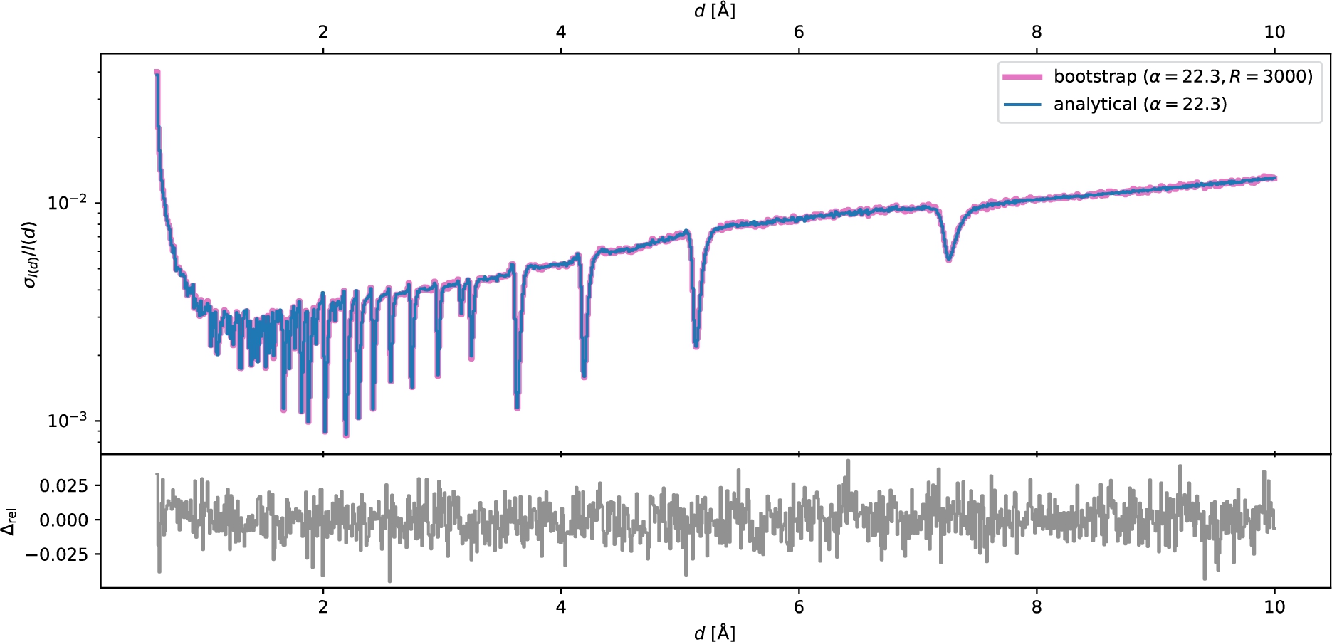
In Fig. 6 we compare the relative errors computed using the analytical approach and bootstrap (see Appendix A, in particular Fig. 9 which shows the same result for
Fig. 7.
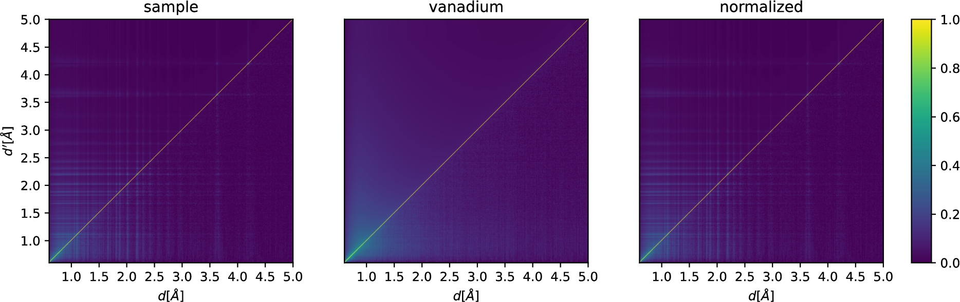
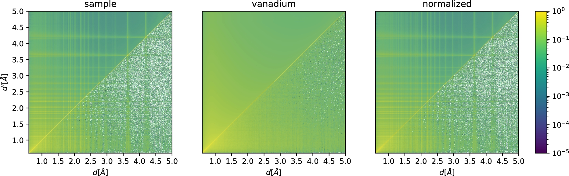
Correlation matrices for a powder-reduction workflow. We show the result for the sample S (left,
3.3.Vanadium normalization
For scattering off a vanadium sample, we define
3.4.The effect of smoothing
Smoothing is routinely used to reduce the effect of noise in normalization terms such as a neutron monitor spectrum or a reduced vanadium spectrum. This reduces the size of the variances of the normalization term,1919 and thus the relative importance of these uncertainties when combined with the variances of the detector counts. However, the smoothing procedure introduces additional correlations between bins of the normalization term which counterbalance the effect. Smoothing can be described as a convolution with a kernel function
4.Discussion
4.1.Current software: Scope and impact of incorrect uncertainty handling
We have described and demonstrated a systematic problem with the treatment of the statistical uncertainties of normalizations terms in Mantid and Scipp. This constitutes the most important result of this work.
Affected software includes Mantid (all versions at the time of writing, at least up to Mantid v6.5) and Scipp (all versions up to Scipp v22.11, inclusively) but the issue may also be present in other similar data-reduction software. Mantid is used at the ISIS Neutron and Muon Source at the STFC Rutherford Appleton Laboratory (http://www.isis.stfc.ac.uk/), the Spallation Neutron Source (SNS) and the High Flux Isotope Reactor (HFIR) at the Oak Ridge National Laboratory (http://neutrons.ornl.gov/), the Institut Laue-Langevin (ILL, https://www.ill.eu/), the China Spallation Neutron Source (CSNS, http://english.ihep.cas.cn/csns/), the European Spallation Source ERIC (ESS, http://europeanspallationsource.se/), the Forschungs-Neutronenquelle Heinz Maier-Leibnitz (FRM II, https://www.frm2.tum.de/en/frm2/home/), and SINQ at the Paul Scherrer Institute ( https://www.psi.ch/en/sinq). Scipp is used at the ESS. All experimental techniques, including powder-diffraction, small-angle scattering, reflectometry, single-crystal diffraction, spectroscopy, and imaging can be affected. Many data-reduction workflows are affected multiple times. For example, in powder diffraction we may perform normalization of sample data to monitor (problem from broadcast over pixels and event-mode), normalization of vanadium data to monitor (problem from broadcast over pixels and event-mode), normalization of reduced data to vanadium (problem from event-mode). Even this relatively simple example includes five distinct instances of the problem.
To our knowledge little or no impact of the issue described in this manuscript has been reported in practice. There are at least two likely explanations. Firstly, variations of Eq. (13) may hold in many cases. That is, in practice the normalization terms often have very good statistics – as we have seen for the concrete SANS and powder diffraction examples in Section 3.1 and Section 3.2, respectively. This can be both due to practicality (it is relatively simple to measure many vanadium counts, or have a monitor with a high count rate) and due experience (instrument scientists know how long to measure normalization terms for good results). Secondly, coordinate transformations, as well as preprocessing steps of the normalization terms such as smoothing, lead to correlations that spread over a wider range. These correlations might affect mostly non-local aspects, which could be harder to discern when, e.g., fitting a physical model to the reduced result.2020
In our opinion the above can however not justify dismissal of the issue. The current state-of-the-art software gives a false sense of security (of having handled uncertainties correctly) to the scientist. While we managed to compute corrected analytical results for variances and covariances in the model workflows used in this manuscript, this cannot be directly substituted in CS implementations for the operation-by-operation error-propagation mechanism. At the very least our software must thus avoid giving a false sense of security and should therefore reject normalization terms that have uncertainties. This will force the scientist to consider whether the normalization uncertainties fulfill Eq. (13). Based on this they can then either (A) confidently drop this term or (B) increase the statistics by measuring the normalization terms better.
A complete analysis for any particular technique such as SANS or powder-diffraction is beyond the scope of this manuscript. The workflows discussed in Section 3 are therefore not necessarily capturing all potential sources of uncertainties, but are meant to illustrate the key aspects. To give an idea of what a more complete analysis might involve, consider the SANS case. Our analysis in Section 3.1 covered the effects of the variances of the monitors. There are however a number of other contributions: (1) Before computation of wavelengths and Q, the beam center is determined. The uncertainty on the beam center leads to a correlation of all computed wavelength and Q values. (2) For the computation of the transmission fraction, each monitor is background-subtracted: The monitor background is computed as the mean over a user-defined wavelength range and then subtracted from the monitor. This broadcasts the mean value to all monitor bins, leading to correlations. (3) The direct beam function D itself comes with uncertainties which were computed using CS and may thus be underestimated in themselves.
Intriguingly, the SANS data reduction implemented in Scipp prior to this work (and used for this analysis) actually ignored the uncertainties of D. This provides a worrysome glimpse of the potentially cascading negative effects of the CS implementation: An interpolation is required to map D to the wavelength-binning of the monitors, and it was unclear how uncertainties should be handled during this interpolation. During development of the workflow it was determined empirically that setting D’s uncertainties to zero had no influence on the uncertainties of the final result. Looking back, we can now tell that this empiric evidence was based on the incorrect handling of uncertainties – since the broadcast of the pixel-independent D to all pixels supresses its contribution to the final uncertainties. Thus the decision to ignore them needs to be revisited. Preliminary results indicate that correct handling of the uncertainties of D may noticably impact the final uncertainties.
4.2.Improved analytical approach
Aside from highlighting the systematic problem, we have succeeded in Section 3 in deriving expressions for variance-covariance matrices of the data-reduction results. As we will show in the discussion in Section 4.3, there is likely no major difference in terms of computational cost compared to the flawed approach currently implemented in Mantid and Scipp, even though it provides access to not just the variances but also the covariances of the final result. We conjecture that our approach may be feasible also for complete and realistic data-reduction workflows. We plan to investigate this in more detail in future work, in particular to extend this to other neutron-scattering techniques and to include corrections such as absorption corrections and background subtractions.
A fundamental difference – and possibly the main challenge – is that unlike in the CS implementation, handling and computation of variances is difficult to automate. While Python packages such as JAX [4] and Uncertainties [16] implement automatic differentiation approaches, it is unlikely that this is directly applicable for the components of a neutron-scattering data-reduction workflow.2121 That is, we would need to either rely on fixed workflows with previously derived expressions for the variance-covariance matrix, or the user must derive these on their own. If a user does derive such an expression, programming skills are required to implement it. In either case, workflows that handle error propagation may become less interactive.
On the positive side, our new approach can produce data-reduction results including covariances. This may be beneficial for subsequent analysis and model fitting procedures. Furthermore, Scipp has proven flexible enough to allow for computation of the expressions for the variance-covariance matrix with very concise code and adequate performance. This further increases our confidence that the described approach may be a viable solution for handling data from day-to-day instrument operations.
4.3.Computational cost of the improved analytical approach
In Sections 3.1 and 3.2 we described an improved analytical approach for computing uncertainties and correlations for the result of the data-reduction. The computation of the variance-covariance matrices turns out to be not significantly more expensive than the computation of the cross sections. Despite yielding the full correlation matrix the overall cost is thus comparable to that of the CS implementation. This holds true even for event-mode data-reduction. To understand this, one important aspect to realize is that – in contrast to CS – it is no longer necessary to carry the uncertainties of the detector counts in intermediate steps, since for the raw input data the variances are equal to the measured counts. A full analysis of the performance characteristics is beyond the scope of this paper. We briefly touch on the main aspects and proceed to report concrete timings for an example below.
Firstly, considering the normalization operation we observe the following. In addition to the normalized counts,
We illustrate this on the example of the Wish powder-diffraction data-reduction. The input data has a file size of
Table 1
Timings for the relevant part of the Wish histogram-mode data-reduction.
| CS [s] | ours [s] | |
| 1000 | 1.8 | 2.3 |
| 2000 | 3.3 | 4.5 |
| 4000 | 6.3 | 10.9 |
5.Conclusion
In this paper we have shown a systematic problem with the treatment of the statistical uncertainties of normalizations terms in Mantid and Scipp. We have shared our findings with the Mantid development team. In the Scipp project, we have disabled propagation of uncertainties if one of the operands is broadcast in an operation with the release of Scipp v23.01. Support for event-mode normalization operations with normalization terms that have variances is also disabled. In both cases an exception is raised instead, i.e., the operation will fail, forcing the user to address the problem correctly. We had initially considered simply displaying a warning to the user when an operation introduces correlations. However, experience shows that warnings are almost always ignored and we now do not consider such an approach as a solution.
Aside from highlighting the systematic problem, we have succeeded in deriving expressions for variance-covariance matrices of the data-reduction results. Computationally the new approach would be feasible, but whether it is applicable and useful in practice remains to be investigated.
Notes
1 Disclaimer: The authors of the present paper are the principal authors of Scipp and have previously contributed to Mantid for several years.
2 The normalization term could be, e.g., a neutron monitor spectrum or a reduced vanadium spectrum.
3 Whether this assumption is always correct is not the topic of this manuscript.
4 Here we chose to compute the same result in two steps using correlations of summands since it aids in highlighting the difference to the CS approach. A direct and likely simpler way to compute this is using
5 Multiplication
6 In Mantid such coordinate transformations are referred to as unit conversion.
7 The direct-beam function allows to cross-normalize the incident spectrum to that of the empty beam (without sample) seen on the main detector.
8 Here we assumed quasi-elastic scattering. A correction factor for inelastic-scattering [14] would depend on i, j, and λ.
9 The data has been published in [17], where all the details on the experimental setup can be found.
10 The monitors from the direct run,
11 For related methods such as Markov-chain Monte-Carlo uncertainty estimates see, e.g., Ref. [2] and [18].
12 Including background subtraction in our bootstrap calculations, i.e., computing
13 We use bins of constant width to simplify the notation, but the following results are equally valid for other choices of bin widths.
14 Note that in software histogramming is not actually implemented via a matrix multiplication as this would be highly inefficient.
15 For example, scipy.optmize.curve_fit accepts the covariance matrix as input via the sigma parameter. A full discussion for other approaches such as Bayesian statistics is beyond the scope of this paper.
16 The sample is NaCaAlF measured in Wish run number 52889 and the vanadium was measured in run number 52920.
17 We use bins of constant width for simplifying the notation, but the following results are also valid for other choices of bin widths.
18 For histogrammed data the expression may need to be adapted depending on the rebinning approach that is being used.
19 Note that, e.g., Mantid’s FFTSmooth (version 2) algorithm sets uncertainties directly to 0. This behavior appears to be undocumented.
20 We do not have enough background knowledge about concrete subsequent data analysis methods to tell when and where such non-local properties might be irrelevant.
21 Even if automatic differentiation could handle operations such as histogramming, the Uncertainties Python package stores arrays with uncertainties as arrays of values with uncertainties. The very high memory and compute overhead makes this unsuitable for our needs.
22 Timings measured for NumPy [10] backed by a multi-threaded linear-algebra library.
23 This assumption also underlies the regular propagation of uncertainties.
Acknowledgements
We kindly thank the authors of Ref. [17] for allowing us to use their data for the SANS example. We thank Pascal Manuel for sharing Wish data, used in our powder-diffraction example. We thank Evan Berkowitz and Thomas Luu for valuable discussions about bootstrap and correlations. We thank our coworkers Celine Durniak, Torben Nielsen, and Wojciech Potrzebowski for helpful discussions and comments that helped to improve the clarity of the manuscript.
Appendices
Appendix A.
Appendix A.Bootstrap
This section gives a brief overview of bootstrapping as used in this work. For a more complete explanation we refer to Ref. [9]. Given a measured distribution of random variables
In this work,
Fig. 8.
Convergence of bootstrap to the analytical result for the relative standard deviation for SANS
We assume all
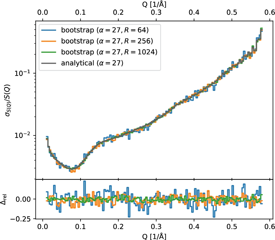
As an example, Figs 8 and 9 show the relative standard deviation of
Fig. 9.
Convergence of bootstrap to the analytical result for the relative standard deviation for powder diffraction
Appendix B.
Appendix B.Figures for correlation matrices
For completeness, we show in this section the figures of the correlation matrices from the SANS and powder diffraction workflows using a logarithmic color scale.
Fig. 10.
Correlation matrices for the time-of-flight SANS-reduction workflow using
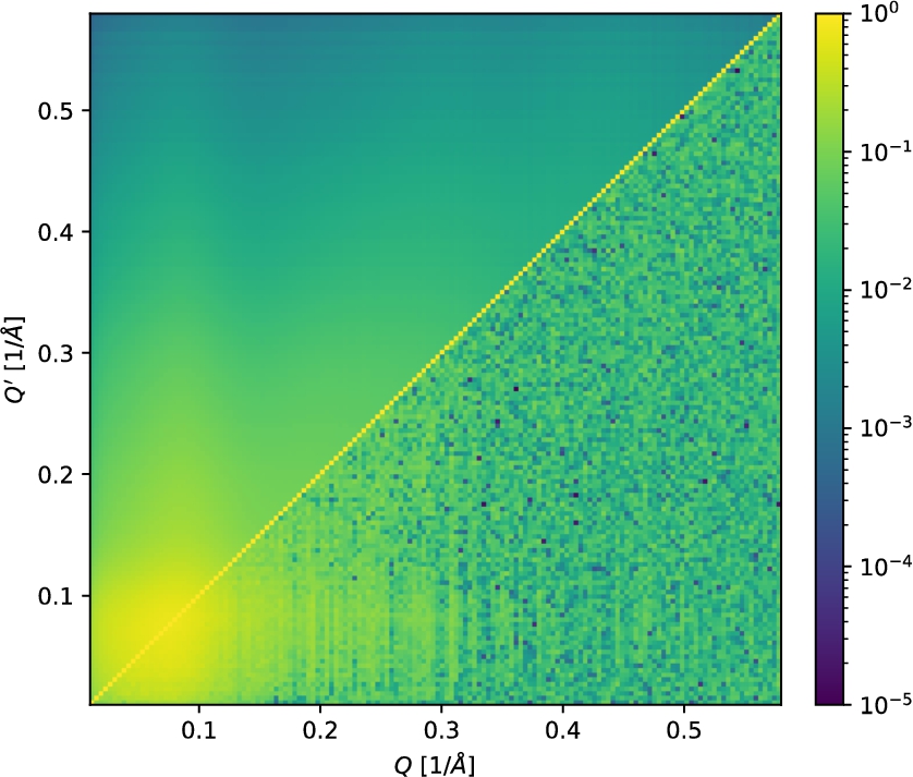
Fig. 11.
Correlation matrices for a powder-reduction workflow. We show the result for the sample S (left,
References
[1] | O. Arnold, J.C. Bilheux, J.M. Borreguero, A. Buts, S.I. Campbell, L. Chapon, M. Doucet, N. Draper, R.F. Leal, M.A. Gigg, V.E. Lynch, A. Markvardsen, D.J. Mikkelson, R.L. Mikkelson, R. Miller, K. Palmen, P. Parker, G. Passos, T.G. Perring, P.F. Peterson, S. Ren, M.A. Reuter, A.T. Savici, J.W. Taylor, R.J. Taylor, R. Tolchenov, W. Zhou and J. Zikovsky, Mantid – data analysis and visualization package for neutron scattering and μSR experiments, Nuclear Instruments and Methods in Physics Research Section A: Accelerators, Spectrometers, Detectors and Associated Equipment 764: ((2014) ), 156–166. doi:10.1016/j.nima.2014.07.029. |
[2] | B.A. Berg, Introduction to Markov Chain Monte Carlo Simulations and Their Statistical Analysis, (2004) . doi:10.48550/ARXIV.COND-MAT/0410490. |
[3] | P.R. Bevington and D.K. Robinson, Data Reduction and Error Analysis for the Physical Sciences, McGraw-Hill, Boston, (2003) . |
[4] | J. Bradbury, R. Frostig, P. Hawkins, M.J. Johnson, C. Leary, D. Maclaurin, G. Necula, A. Paszke, J. VanderPlas, S. Wanderman-Milne and Q. Zhang, JAX: Composable transformations of Python+NumPy programs, 2018, http://github.com/google/jax. |
[5] | Broadcasting in NumPy, https://numpy.org/doc/stable/user/basics.broadcasting.html. |
[6] | L. Chapon, P. Manuel, P. Radaelli, C. Benson, L. Perrott, S. Ansell, N. Rhodes, D. Raspino, D.M. Duxbury, E. Spill and J. Norris, Wish: The new powder and single crystal magnetic diffractometer on the second target station, Neutron News 22: ((2011) ), 22–25. doi:10.1080/10448632.2011.569650. |
[7] | Documentation of error propagation in Mantid, 2022, https://docs.mantidproject.org/nightly/concepts/ErrorPropagation.html. |
[8] | U. Drepper, What Every Programmer Should Know About Memory, 2007, https://people.freebsd.org/~lstewart/articles/cpumemory.pdf. |
[9] | B. Efron and R.J. Tibshirani, An Introduction to the Bootstrap, Chapman and Hall/CRC, (1994) . doi:10.1201/9780429246593. |
[10] | C.R. Harris, K.J. Millman, S.J. van der Walt, R. Gommers, P. Virtanen, D. Cournapeau, E. Wieser, J. Taylor, S. Berg, N.J. Smith, R. Kern, M. Picus, S. Hoyer, M.H. van Kerkwijk, M. Brett, A. Haldane, J.F. del Río, M. Wiebe, P. Peterson, P. Gérard-Marchant, K. Sheppard, T. Reddy, W. Weckesser, H. Abbasi, C. Gohlke and T.E. Oliphant, Array programming with NumPy, Nature 585: (7825) ((2020) ), 357–362. doi:10.1038/s41586-020-2649-2. |
[11] | R.K. Heenan, J. Penfold and S.M. King, SANS at pulsed neutron sources: Present and future prospects, Journal of Applied Crystallography 30: (6) ((1997) ), 1140–1147. doi:10.1107/S0021889897002173. |
[12] | S. Heybrock, O. Arnold, I. Gudich, D. Nixon and N. Vaytet, Scipp: Scientific data handling with labeled multi-dimensional arrays for C |
[13] | S. Heybrock, N. Vaytet and J.-L. Wynen, Systematic underestimation of uncertainties by widespread neutron-scattering data-reduction software – Supplementary Material, Zenodo, 2023. doi:10.5281/zenodo.7708115. |
[14] | R. Hjelm, The resolution of TOF low-Q diffractometers: Instrumental, data acquisition and reduction factors, Journal of Applied Crystallography 21: ((1988) ), 618–628. doi:10.1107/S0021889888005229. |
[15] | ISIS Powder Diffraction Scripts Workflow Diagrams, https://docs.mantidproject.org/v6.5.0/techniques/ISISPowder-Workflows-v1.html. |
[16] | O.E. Lebigot, Uncertainties: A Python package for calculations with uncertainties, 2023, http://pythonhosted.org/uncertainties/. |
[17] | I. Manasi, M.R. Andalibi, R.S. Atri, J. Hooton, S.E.M. King and K.J. Edler, Self-assembly of ionic and non-ionic surfactants in type IV cerium nitrate and urea based deep eutectic solvent, The Journal of Chemical Physics 155: (8) ((2021) ), 084902. doi:10.1063/5.0059238. |
[18] | C.E. Papadopoulos and H. Yeung, Uncertainty estimation and Monte Carlo simulation method, Flow Measurement and Instrumentation 12: (4) ((2001) ), 291–298. doi:10.1016/S0955-5986(01)00015-2. |
[19] | P.F. Peterson, S.I. Campbell, M.A. Reuter, R.J. Taylor and J. Zikovsky, Event-based processing of neutron scattering data, Nuclear Instruments and Methods in Physics Research Section A: Accelerators, Spectrometers, Detectors and Associated Equipment 803: ((2015) ), 24–28. doi:10.1016/j.nima.2015.09.016. |
[20] | P.F. Peterson, D. Olds, A.T. Savici and W. Zhou, Advances in utilizing event based data structures for neutron scattering experiments, Review of Scientific Instruments 89: (9) ((2018) ), 093001. doi:10.1063/1.5034782. |
[21] | Sans2d: I(Q) workflow for a single run (sample), https://scipp.github.io/ess/instruments/loki/sans2d_to_I_of_Q.html. |
[22] | Sans2d: Time-of-flight Small-Angle Neutron Scattering instrument, https://www.isis.stfc.ac.uk/Pages/Sans2d.aspx. |
[23] | Scipp Documentation, 2022, https://scipp.github.io/. |
[24] | SNSPowderReduction algorithm documentation, https://docs.mantidproject.org/v6.5.0/algorithms/SNSPowderReduction-v1.html. |


