
Research of news text classification method based on hierarchical semantics and prior correction
Abstract
News text is an important branch of natural language processing. Compared to ordinary texts, news text has significant economic and scientific value. The characteristics of news text include structural hierarchy, diverse label categories, and limited high-quality annotation samples. Many machine learning and deep learning methods exist to analyze various forms of news text. However, due to label imbalance, hierarchical semantics, and confusing labels, current methods have limitations. Therefore, this paper proposes a news text classification framework based on hierarchical semantics and prior correction (HSPC). Firstly, data augmentation is used to enhance the diversity of the training set and adversarial learning is employed to improve the resistance of the model with its robustness. Then, a hierarchical feature extraction approach is employed to extract semantic features from different levels of news texts. Consequentially, a feature fusion method is designed to allow the model to focus on relevant hierarchical semantics for label classification. Finally, highly confusing label predictions are corrected to optimize the label prediction of the model and improve confidence. Multiple experiments are performed on four widely used public datasets. The experimental results indicate that HSPC achieves higher classification accuracy compared to other models. On the FCT, AGNews, THUCNews, and Ohsumed datasets, HSPC improves the accuracy by 1.03%, 1.38%, 2.55%, and 1.15%, respectively, compared to state-of-the-art methods. This validates the rationality and effectiveness of the designed mechanisms.
1Introduction
Text classification is an important task in natural language processing and plays a significant role in various applications such as topic labeling [1], sentiment analysis [2], and textual similarity analysis[3]. In the age of information, news classification has become a vital research field in text classification due to the rapidly increasing amount of data on the internet. The goal of news text classification is to assign the most appropriate text label to news articles with unknown labels and it is widely applied in news topic identification [4], user news recommendation [5] and news polarity analysis [6]. Compared to other types of texts, news text holds greater economic value and scientific research value. On the one hand, by categorizing news articles, decision-makers can better understand public opinion and analyze the dynamics of society and the public opinion environment. On the other hand, news text classification helps organize and retrieve massive news texts. Users can more conveniently and effectively access news content of interest. Based on users’ reading preferences, researchers can recommend personalized news services on their favorite topics. Accordingly, it is essential to categorize new text to improve user experience, reduce information acquisition costs, and analyze the media coverage.
There are several methods available for text classification. An early optimal solution involves using knowledge engineering for classification. However, this method requires significant human and material resources, has limited application coverage, and achieves low classification accuracy.
Therefore, researchers propose using traditional machine learning methods. For example, there are text classification methods based on the K-nearest neighbors algorithm such as [7, 8] and based on support vector machines including [9–11]. In recent years, many papers have used a variety of machine learning algorithms for news text classification to explore the most appropriate approach for a particular domain [12–15]. Among them, Sidar [12] uses 41 diverse machine learning algorithms to classify 4000 news articles in specific domains, successfully showcasing the potential of various machine learning algorithms. However, machine learning has some inevitable limitations. One of the main challenges is that news text is highly flexible in its use of language. Even sentences with the same meaning can be expressed differently in different news texts. Compared to ordinary text, this means that converting news into computer language can result in a greater loss of information. Additionally, traditional machine learning methods may exacerbate the loss through feature engineering. In addition, traditional machine learning methods often struggle to capture order and dependencies between words. It is crucial to create an efficient model that can handle sequences of varying lengths and capture contextual information in text to improve classification performance.
Furthermore, many methods focus on deep learning to conduct new text classification. For example, GRU-CNN [16] combined CNN and GRU to simultaneously extract local features, semantic information, and global structural relationships of news text. Depending on the different model embeddings, character level [17], word level [18] and sentence level [19] have been proposed. As research progresses, researchers have started exploring how to parse semantics using graph structures, including TextING [20] and [21]. With the development of pre-training, pre-trained models such as ERNIE [22, 23] have gradually gained attention. The BERT language model [24] has also been used for generating adversarial samples to assist in text classification [25]. However, the previous works still have some deficiencies as follows. Firstly, there are few high-quality annotated news texts due to the high cost and difficulty of annotation. This leads to label imbalance and insufficient training set when using the dataset for training classification models. Secondly, news articles have a specific style of writing, with diverse semantic levels to meet the unique needs of the industry. However, most current methods use holistic feature extraction methods, which do not fully utilize the hierarchical semantics of news texts. This leads to one-sidedness when parsing the semantic features of news texts. Thirdly, News texts within the intersection range of multiple fields can be attributed to different label categories. The greater differences between label scores lead to lower confusion and higher confidence in classification results. Nevertheless, existing text classification models overlook the impact of predictions for highly confusing labels and do not make corrections for such labels.
To address the issues mentioned above, this paper proposes a news text classification framework based on Hierarchical Semantics and Prior Correction (HSPC). Firstly, in responding to insufficient data and imbalanced labels, HSPC leverages data augmentation technology and adversarial learning to improve the sample diversity of news text data and optimize the model training effect further. Then, considering the influence of strongly related words of labels in the news body and the hierarchical semantic difference between the news title and news body, the pre-trained model and the deep learning model are used to obtain the features of different levels. Subsequently, text features at various levels are integrated to obtain the final features of the news text. Finally, a prediction correction algorithm based on the prior distribution (PD) is designed to adjust the result of label predictions and improve the accuracy of news text classification.
To summarize, the contributions of this paper are as follows:
1. This paper proposes data enhancement for improving the quality of the dataset and adversarial learning for improving the anti-interference ability of the model in the model training process.
2. Due to the hierarchical semantic differences in news articles, the feature representations of news titles and news bodies are extracted separately. Then, an adaptive gating mechanism is used to fuse the text features of two different levels, so that the model can focus more on the semantic hierarchy associated with news labels.
3. A correction algorithm based on prior distribution is designed, which corrects the predicted distribution of highly confusing labels. This alleviates the impact of label probability confusion and enhances confidence in model label predictions.
The rest of the paper is organized as follows. Section 2 introduces the key techniques of the news text classification framework based on hierarchical semantics and prior correction. Section 3 presents the experimental settings and results, including comparative experiments, ablation experiments, and correction analysis experiments. Section 4 summarizes the research content of this paper. It also points out the limitations of the proposed research approach and provides prospects for future research in the field of news text classification methods.
2Materials and methods
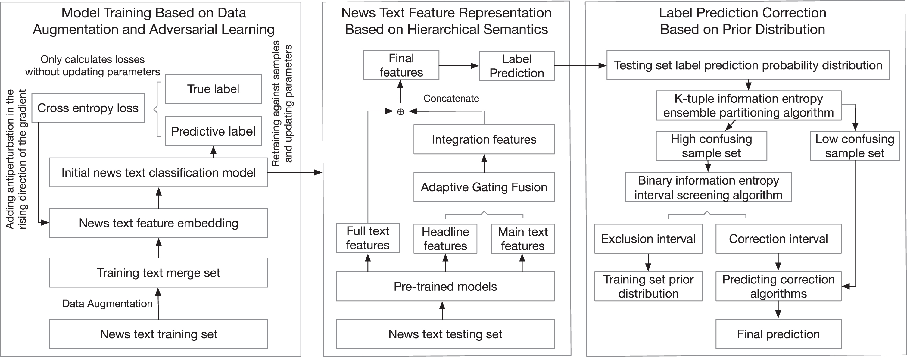
In this section, HSPC is introduced, which comprises three primary components: model training based on data augmentation and adversarial learning, news text feature representation based on hierarchical semantics, and label prediction correction based on prior distribution. The model framework is illustrated in Fig. 1.
Fig. 1
Overall framework of news text classification.
2.1Model training based on data augmentation and adversarial learning
The key to successful model training is a high-quality dataset that reduces the likelihood of overfitting. As part of the model training process, adversarial learning is introduced to enhance its robustness and strengthen its resistance to interference.
2.1.1Data augmentation
First, the dataset is optimized through data augmentation by generating diverse augmented texts with different sentence structures using a multilingual translation approach. This enhances the quality of the simple news titles. Specifically, the text is translated into other languages using a translator. Then, the translated titles are back-translated to generate augmented titles that resemble the original text. These augmented titles serve as additional training data for news titles.
The news body is typically a long and complex text with intricate sentence structures. To avoid sentence structure disorder, a data augmentation method based on keyword avoidance and synonym replacement is employed to transform the news body text. The specific steps involve building a synonym table, generating a keyword dictionary for the news body, and performing random synonym replacement. To construct the synonym table, all the vocabulary in the dataset is extracted. Then, by querying a word vector table, the top k synonyms with cosine similarity greater than the threshold are selected for each word, forming a synonym word list. The process of calculating cosine similarity between words is as follows:
(1)
Next, the keyword dictionary for the news body is generated. The TF-IDF correlation coefficients between each word in the dataset and the news body are calculated. From the correlation coefficients, the top m words are selected to form the keyword dictionary for each text. Then, random keyword substitution is performed after tokenizing the input text. About
After acquiring the augmented news bodies and titles, they are merged with the original news text training set to create the final dataset for model training.
2.1.2Optimization of model training based on adversarial learning
In the process of training the news text hierarchical semantic classification model, adversarial learning is employed to improve the model’s robustness and ability to generalize. This is achieved by introducing perturbations in the embedding layer, which makes the training process more challenging and encourages the model to adapt to the influence of perturbations.
Firstly, the model is trained normally with the original samples and the loss is computed using the cross-entropy loss function. This process is shown in the following equation:
(2)
First, the loss is backpropagated to compute the gradient of the loss for the embedding. The gradient is then scaled by a constraint coefficient to control the perturbation magnitude. The equation reads:
(3)
Subsequently, adversarial training learning data is generated by adding the perturbation to the direction of increasing gradient in embedding. It can be expressed as:
(4)
The model is then retrained using the data, and the adversarial loss is computed which is defined as follows:
(5)
Finally, the original model embedding is restored, and the adversarial loss is backpropagated to update the model parameters.
2.2News text feature representation based on hierarchical semantics
Feature representation considers the characteristics of news texts at different semantic levels, using overall full-text characteristics as auxiliary. Specifically, firstly, since news titles have dense label information, CNN is used to extract local text features of news titles. Secondly, considering the semantic complexity of a long news body, BiLSTM is utilized to extract long-distance semantic features. And the model focuses more on the information strongly related to the labels. Next, the adaptive gating mechanism integrates the features of the news title and the features of the news body. The fusion features obtained are then concatenated with the full-text features obtained through the pre-trained model to assist in downstream news text classification tasks. Finally, the feature vectors can be used to obtain prediction scores for each label.
The process of representing news features based on hierarchical semantics primarily involves the extraction of news title features, news body features, the fusion of hierarchical semantic text features, and the prediction of label probabilities.
2.2.1The extraction of news title features
During the extraction of news title features, a pre-trained BERT model is utilized to parse the news titles and obtain the feature matrix titleout. To extract local text features from it, a two-layer convolutional neural network (CNN) is employed to process this feature matrix. Considering multiple dimensions of semantic hierarchy, various convolutional kernels are used to extract features from this matrix. The list of convolutional kernels used is represented as follows:
(6)
where pilterij donates different convolutional kernels. n represents the number of different sizes of convolutional kernels, and m represents the number of convolutional kernels for each size.
Next, a pooling layer is applied to compress the extracted high-dimensional features, filtering out non-key features in the local features of the title. After the compression through convolution and pooling, each high-dimensional feature is concatenated to obtain the news title feature Ftitle.
2.2.2The extraction of news body features
The process of extracting features from the news body text mainly involves long-range feature extraction and document attention fusion. During long-range feature extraction, a pre-trained model BERT is initially used to extract the sequence features of the body text, denoted as contentout. Subsequently, contentout is fed into a Bidirectional Long Short-Term Memory(BiLSTM) to assist in extracting semantic features from long-distance sequences in the body text. The last hidden state HD and the feature matrix ED are given by the following equation:
(7)
(8)
(9)
(10)
(11)
(12)
2.2.3The fusion of hierarchical semantic features
The feature vector Ftitle extracted from the news title feature matrix and the feature vector Fcontent extracted from the news body text feature matrix represent different levels of interpretation of the entire news article, and they have varying influences on the classification of news labels. HSPC uses an adaptive gating network [30] to enable the model to balance the effects of both and select the text semantic level with stronger label relevance. First, the fusion proportion is computed. The process is shown in the following formula:
(13)
Next, G is used to perform a weighted sum of the news title feature vector Ftitle and the news body text feature vector Fcontent, resulting in the complete feature vector Fnew_gates for the full news text. The process is illustrated in the equation as follows:
(14)
After that, a pre-trained model is used to extract the full-text feature vector Fnew_pre from the entire news article. Then, a linear concatenation is performed between Fnew_pre and Fnew_gates to assist Fnew_gates in text classification. The formula is demonstrated as follows:
(15)
2.2.4the prediction of label probabilities
After obtaining the final news text representation vector Fnews, it is converted into probability scores out for the labels. The vector space mapping is defined as follows:
(16)
Then, out is normalized to obtain the probability of the text representation vector belonging to each label. The label with the highest probability is selected as the best label for the news text. The process is defined as follows:
(17)
where softmax represents the normalization operation and pred represents the label prediction distribution.
2.3Label prediction correction based on prior distribution
In news text classification, the accuracy of predicted labels is affected by the level of confusion in the label prediction distribution. To improve accuracy, it’s necessary to correct predictions for labels with high confusion. This correction process involves three steps. Firstly, the confusion prediction set is divided into high and low confusing sample sets using K-entropy partitioning. Secondly, label correction intervals are selected based on binary entropy to filter out intervals that need to be corrected in highly confusing sample sets. Thirdly, label prediction correction is done based on prior distribution, where the probability distribution of the statistical labels in the training set is used as a prior distribution. This prior distribution adjusts the correction interval for each highly confusing sample.
2.3.1Confusion prediction set partitioning based on K-entropy
By utilizing the top k highest label prediction probabilities, the confusion score of the predicted label for a news test sample is calculated. Assuming p1, p2, p3, …, pk are the k highest probability scores, the first step is to normalize these k probability values. The normalization process is defined as follows:
(18)
Next, the K-entropy is calculated as the confusion score, expressed as pred _ S:
(19)
Algorithm 1 Confusion prediction set partitioning based on K-entropy
Input: probability distribution set of the news test dataset test _ pred; set partition threshold t; top k parameter k.
Output: set of low confusing sample distributions clear; set of highly confusing sample distributions confused.
1: Function set partitontest _ pred, k, t
2: confused = [] , clear = []
3: For pred in test _ pred do
4: pred _ top _ k = sort (pred, k)
5: pred _ top _ k = normalize (pred _ top _ k)
6: pred _ S = S (pred _ top _ k)
7: if pred _ S > t then
8: confused . append (pred _ top _ k)
9: else
10: clear . append (pred _ top _ k)
11: return confused, clear
The confusion partition algorithm is shown in Algorithm 1. The algorithm takes inputs including the probability distribution set of the news test dataset test _ pred, the set partition threshold t, and the top k parameter. It outputs two sets: clear for low confusing sample distributions and confused for highly confusing sample distributions. First, two new probability distribution lists, confused and clear, are initialized to store the partitioned highly confusing and low confusing label predictions, respectively (line 2). Next, iterate over each sample distribution in the test dataset and retrieve the top k highest probability scores from the distribution (lines 3-4). After re-normalizing the scores, calculate the K-entropy as the confusion score for the distribution (lines 5-6). The formula for information entropy S is shown in the following equation:
(20)
Then, partition the distribution into the highly confusing sample set if its confusion score exceeds the threshold. Otherwise, assign the distribution to the low confusing sample set (lines 7-10). Finally, output the partitioned highly confusing label prediction set confused and low confusing label prediction set clear.
Next, the time complexity and space complexity of the partitioning algorithm are analyzed. When the training set size is n, the algorithm time complexity of the traversal operation is O (n). If m is the number of labels, the complexity of calculating k-element information entropy is O (m). Moreover, the algorithm for the comparison operation has a time complexity of O (1). Sorting each testing set distribution has a time complexity of O (mlogm). Therefore the total time complexity is O (nmlogm). For space complexity, the additional space is two lists confused and clear. The sum of samples in the list is the number of samples in the training set n. Each sample contains label predictions of length m. Finally, extra space O (nm) is required.
2.3.2Label correction interval selection based on binary entropy
After partitioning the set, the highly confusing label prediction set confused and the low confusing label prediction set clear are obtained. To improve the stability of the correction, it is important to further partition the probability correction interval from the confused set. To do this, the label predictions are sorted in descending order based on their probabilities. For simplicity, the sorted probabilities are denoted as shown in the equation:
(21)
To improve the accuracy of predictions, it is often necessary to divide the predicted label distribution into two sub-intervals using a threshold point t. The sub-intervals are the correction interval, denoted as pselect, which lies on the left side of the threshold, and the exclusion interval, denoted as pnoselect, which lies on the right side of the threshold. When partitioning the original label distribution using the threshold point, certain constraints must be satisfied in combinatorial form as follows:
(22)
Algorithm 2 Label correction interval selection based on binary entropy
Input: set of high confused probability distributions confused; interval filtering threshold i.
Output: low confused interval filtering query dictionary pred _ dic.
1: function interval_filteringconfused, i
2: pred _ dic = []
3: for pred in confused do
4: pred _ dic [pred] = []
5: sort _ idx = sort (pred)
6: sum = 0
7: for idx in sort _ idx do
8: pred _ dic [pred] . append (idx)
9: sum = sum + pred [idx]
10: if sum < (1 - sum) then
11: continue
12: S = get _ entropy (sum, 1 - sum)
13: if S ≤ i then
14: break
15: return pred _ dic
Algorithm 2 is used for the interval selection. The input of this algorithm is a set of samples that have been partitioned and is highly confusing. The output of this algorithm is a query dictionary that contains correction intervals. The keys of this dictionary are the predicted label distributions of highly confusing samples, and the values are the corresponding correction intervals for probability distributions. Initially, an empty dictionary pred _ dic is created to store the distribution-corresponding correction intervals (line 2). Then, for each highly confusing sample interval, the pred is sorted in descending order (lines 4-5). The pred _ sum variable is initialized, and the correction interval probabilities are accumulated for each boundary point of the probability distribution (lines 6-9). Next, the correction intervals are checked to see if they satisfy the third and fourth inequality conditions to determine if further filtering is needed (lines 10-14). Finally, the query dictionary pred _ dic is returned.
Next, the time complexity and space complexity of the screening algorithm are analyzed. For time complexity, the algorithm goes through each highly confusing interval sample. If there are n samples, the time complexity of this loop would be O (n). Assuming there are m labels, it would require O (m) time complexity to go through all subscripts of the prediction distribution. Lastly, every testing set distribution needs to be sorted, and the time complexity of this step is O (mlogm). Therefore, the time complexity of the interval screening algorithm is O (nmlogm). Space complexity analysis involves calculating the additional space used by algorithm 2. In this case, the algorithm uses a data structure pred _ dic, which contains key and value pairs that are proportional to the number of highly confusing label prediction samples. If the scale of samples is denoted by n and the size of each pair depends on the number of labels m, then the algorithm requires extra space of O (nm).
2.3.3Label prediction correction based on prior distribution
After determining the correction intervals for each confused prediction, the correction intervals for each set are adjusted using the prior distribution. The specific correction steps can be divided into prior distribution statistics and prior correction. During prior distribution statistics, the prior distribution is calculated by counting the occurrences of each label in the training set and normalizing them. The formula is demonstrated as follows:
(23)
(24)
During the prior correction, firstly, the average distribution of high and low confusing labels is calculated as follows:
(25)
Simultaneously,
(26)
The text step involves re-normalizing
(27)
After the correction, the sum of probabilities in the original correction interval may change, and it may not necessarily add up to 1 when combined with the probabilities outside the correction interval. Therefore, it is necessary to rescale each recalculated label score to embed it back into the original label prediction distribution, ensuring that the sum of scores for all labels in the original distribution is 1. The rescaling process is shown as follows:
(28)
After obtaining the corrected label predictions for the highly confusing samples, the corrected predictions for the highly confusing samples are combined with the label predictions for the low confusing samples to form the final prediction. The label with the highest probability score in each prediction is selected as the final label for the news text.
The calibration algorithm is shown in Algorithm 3. The input to the algorithm includes the query dictionary pred _ dic, the set of low confusing label prediction distributions clear, the set of highly confusing label prediction distributions confused, and the news training set train _ set. The output is the calibrated highly confusing probability distribution of the news text fixed _ confused. First, the algorithm initializes the arrays for the prior distribution and the list for the corrected output probabilities (lines 2-3). Then, the number of labels after frequency counting is normalized, and train _ distri stores the proportion of each label in the training set (lines 4-6). Next, the algorithm iterates through each label prediction distribution in the set of highly confusing samples and performs calibration and re-normalization. The corrected label prediction distribution is then rescaled and embedded back into the original label prediction. The calibration results are stored in the fixed _ confused list (lines 7-11). Finally, the algorithm returns the list of calibrated label predictions, fixed _ confused.
Then the time complexity of the correction algorithm will be analyzed. When the number of training set samples is n and the number of labels is m, the time complexity of calculating the prior probability distribution is O (n). During the correction process, each highly confusing sample needs to be traversed and a prior correction on the label probability within the correction interval needs to be performed. This step has a time complexity of O (nm). Therefore, the time complexity of the correction part is O (nm). The space complexity of the correction algorithm can be analyzed as follows. Algorithm 3 mainly uses two extra spaces, namely traindistribution and fixedconfused. The space complexity for traindistribution is O (n) which means that it is proportional to the number of corrected samples n. The space used by fixedconfused is also proportional to the number of corrected samples, and each label prediction is a vector of length m. Therefore, the space complexity of the correction algorithm is O (nm).
Algorithm 3 Label prediction correction based on prior distribution
Input: query dictionary pred _ dic; set of low confusing label prediction distributions clear; set of highly confusing label prediction distributions confused; training set ts.
Output:calibrated highly confusing probability distribution of the news text fixedconfused.
1: function probability_correction(ts, pred _ dic, clear, confused)
2: tr _ distri = []
3: fixed _ confused = []
4: for label in ts do
5: tr _ distri [lable] = tr _ distri [lable] + 1
6: tr _ distri [lable]/= (sum (lable))
7: for pred in confused do
8: sub _ label = pred _ dic [pred]
9: new _ pred = fix (pred, tr _ distri)
10: new _ pred = handle (new _ pred)
11: fixed _ confused . append (new _ pred)
12: return fixed _ onfused
3Experiments
In this section, comparative experiments, ablation experiments, and calibration analysis experiments are designed to validate the overall classification performance of the HSCP, the effectiveness of various mechanisms within the framework, and the calibration effect of the calibration algorithm.
3.1Experimental Setting
To train the model effectively, the documents in the dataset undergo preprocessing. This involves using a truncation and padding method to ensure that the body text has a uniform character count of 450 and the title has a uniform character count of 30. For data augmentation, the English text is segmented using spaces, and the Glove word vectors of dimension 300 are used for computing synonyms. Chinese text is segmented using the Jieba tokenizer, and the word vector table used is sgns.weibo.word with dimensions of 300.
The parameter settings for the model are as follows: The first layer of the convolutional neural network has three different kernel sizes of length 1, 2, and 4, with a width of 768. The convolutional kernels of the second layer of the convolutional neural network are set to the same length but the widths are all set to 1. The number of kernels for each size is set to 256. The number of convolutional layers is set to 2, and the activation function for each layer is set to ReLU. The hidden layer of the bidirectional long short-term memory network is set to 1, and the dimension of the hidden state feature is set to 768. The number of attention heads is set to 4. Dropout is set to 0.5, and the learning rate is set to 0.001.
The parameters for the calibration algorithm mainly consist of three values. The top-k value which is set to 3, divides the confusing set. The threshold value for dividing the confusing set is set to 0.8 and the threshold value for selecting the correction interval is set to 0.9.
The experimental program was run on the Ubuntu 18.04.4 LTS system. The detailed experimental testing environment is shown in Table 1.
Table 1
Experimental hardware and software configuration
| Software and hardware | Configuration and parameters |
| CPU | Intel i5 9400F |
| GPU | NVIDIA GeForce RTX 2080Ti |
| CUDA | 10.1 |
| Python | 3.6.7 |
| Pytorch | 1.9.0 |
| System | Ubuntu18.04.4LTS |
| Development tool | VS Code |
3.2Dataset
This chapter comprehensively tests the classification performance of HSCP using two Chinese datasets and two English datasets. The specific information and relevant sources of the datasets are as follows:
Fudan Text (FCT) dataset: This dataset is a popular Chinese text classification dataset from the International Database Center for Computer Science at Fudan University, created by their Natural Language Processing group.
THUCNews dataset: The texts in this dataset are obtained by filtering historical data from Sina News by Tsinghua University. A subset of the total dataset is selected for experimentation in this paper.
AG’s News Corpus (AG News): This dataset is a subset of the AG’s news article corpus. It is constructed by combining the title and description fields of articles from the four largest categories: “World,” “Sports,” “Business,” and “Science/Technology.”
Ohsumed dataset: This dataset contains all the cardiovascular disease news reports from 50,216 medical abstracts in 1991. Typically, a subset consisting of titles and abstracts is used for text classification. This subset has a similar structure to news texts and exhibits similar hierarchical semantic characteristics, making it one of the datasets used in this experiment.
The basic attributes of each dataset and the train-test split are shown in Table 2.
Table 2
Data division table
| Datasets | Label category | Sample size of training set | Sample size of testing set | Multilingualism |
| AGNews | 4 | 120 000 | 7 600 | English |
| THUCnews | 13 | 27 300 | 11 700 | Chinese |
| FCT | 20 | 9 804 | 9 833 | Chinese |
| Ohsumed | 23 | 3 357 | 4 043 | English |
3.3Comparative experiments
In this section, the common and effective classification models mentioned in various papers are first introduced. The evaluation metric used in this experiment is accuracy. TextCNN: A text classifier based on convolutional neural networks that extract text features using convolution and compress features using pooling operations to obtain text representations.
LSTM [27]: A method that extracts forward sequence features to classify text, capable of capturing long-distance semantic information in the text.
TextRNN [28]: This method uses recurrent neural networks to process sequential information in text and obtain feature representations of text.
BERT [24]: A bidirectional language model trained on large-scale corpora.
RAM [29]: RAM extracts the radical features of each Chinese character in the news text sentence, vectorizes the information, and combines it with the original character features to enhance the semantic representation of the characters.
AGN [30]: A method integrates the statistical information and feature information of the text through a controlled gate mechanism to assist the text classification model in classification tasks.
TF-GCN [12]: This paper uses LDA topic modeling to obtain the topic distribution of the corpus. Then an algorithm based on a graph convolutional network is used to calculate the learning representation of the combined features for completing the news text classification task.
LCM [31]: With the introduction of label obfuscation, the model is forced to learn more robust feature representations and decision boundaries, which improves the generalization ability of the model.
WTL-CNN [32]: The paper proposes a model that combines word2vec, TF-IDF algorithm and an improved convolutional neural network. Additionally, it takes into account the importance of individual words to the article for improving the accuracy of news text classification.
BERTGCN [33]: This method improves the text classification approach of graph neural networks using pre-trained models.
HyperGAT [34]: The method captures the complex relationships between texts through hypergraph modeling and attention mechanisms to improve the performance of text classification.
Text-level-GCN [35]: It aims at better text classification by building text-level graph structures and applying graph neural networks to capture the relationships between texts.
The characteristics of previous studies compared with HSPC are shown in Table 3. Next, differences will be shown and analyzed between different benchmark methods and HSPC compared on four datasets.
Table 3
Comparison of the characteristics of the main comparison methods on different datasets
| Data | Hierarchical | Label prediction | |
| augmentation | semantics | correction | |
| RAM | ✔ | ||
| AGN | ✔ | ||
| TF-GCN | ✔ | ||
| LCM | ✔ | ||
| WTL-CNN | ✔ | ||
| BERTGCN | |||
| HSPC | ✔ | ✔ | ✔ |
3.3.1Comparison of classification performance for FCT oriented datasets
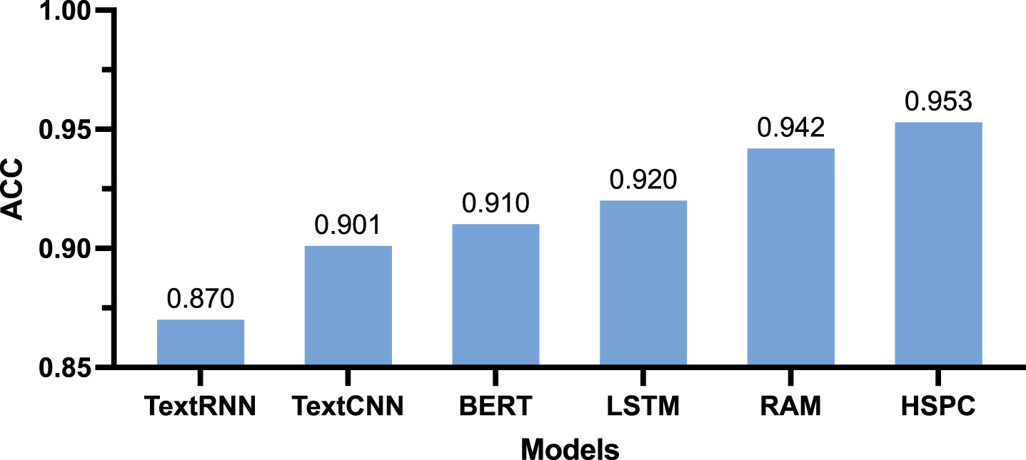
The main comparative method in the FCT dataset is RAM [29]. The classification results of various models on the FCT dataset are shown in Fig. 2. According to the figure, it can be observed that HSPC outperforms the RAM model in terms of classification performance on the FCT dataset. Compared to the RAM model, HSPC shows an improvement of 1.03% in accuracy. This is because news titles often provide a brief yet accurate representation of the news content, making them highly relevant to the news labels. While RAM uses information about the radicals of Chinese characters as semantic extensions, it also introduces redundancy and less relevant information in the process. HSPC takes the title information into separate consideration, allowing the title information to complement the news article information. By specifically considering the title and using it as a semantic expansion of the article, HSPC exhibits a more targeted approach compared to the expansion of news semantics using Chinese character-related intentional information.
Fig. 2
Classification ACC performance comparison chart for FCT dataset.
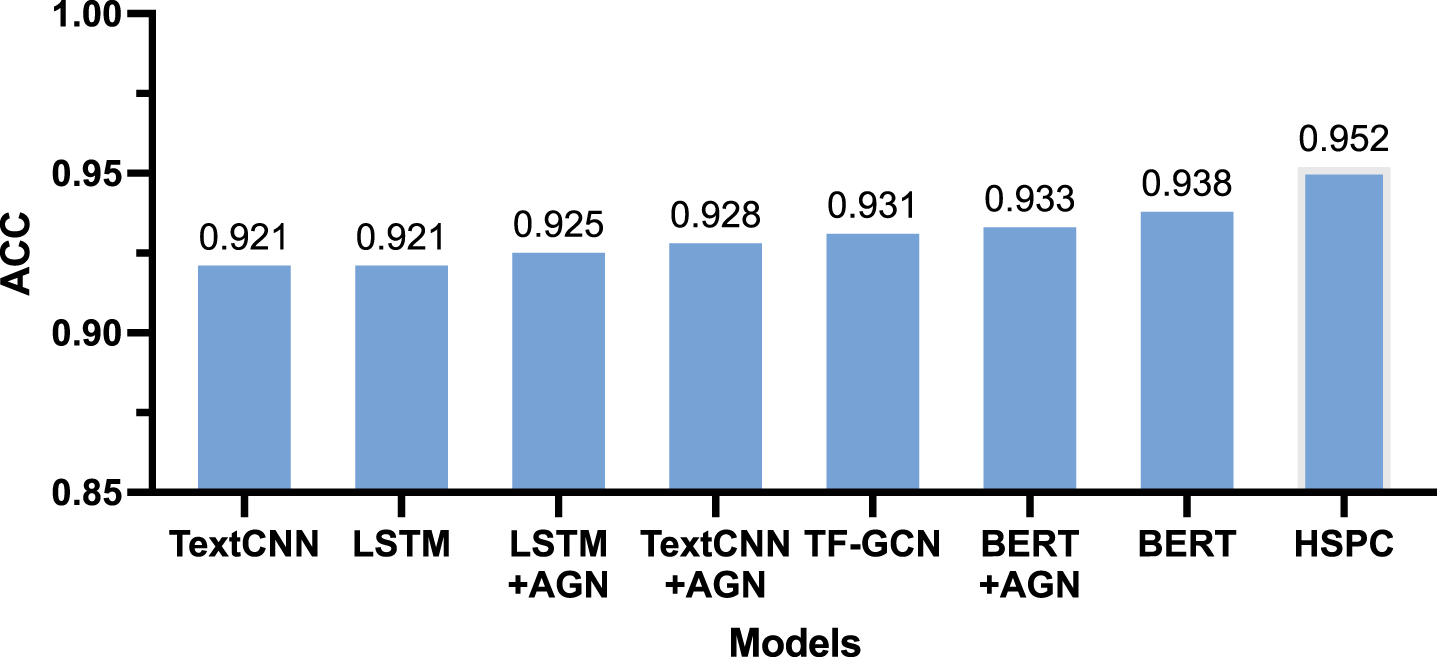
3.3.2Comparison of classification performance for AGNews oriented datasets
The main comparative model in the AGNews dataset is AGN [30] and TF-GCN [12]. Figure 3 provides a comparison of the classification results of various models on the AGNews dataset. According to the figure, it can be observed that HSPC performs better than the BERT+AGN classification model on the AGNews dataset, with an improvement of 1.39% in accuracy. This may be because the primary focus of AGN aims to reduce the influence of less relevant, weakly related, and unrelated words on the labels without extracting more semantic auxiliary feature representations. Meanwhile, the accuracy of HSPC has increased by 2.1% compared to TF-GCN. Although TF-GCN captures three kinds of information including document, topic, and word, as auxiliary information in the heterogeneous information network, it may result in losses when constructing large graphs. In contrast, HSPC considers the hierarchical semantics of news labels separately and uses a gate fusion method to balance the label-level semantics with the article-level semantics. This allows the model to pay more attention to the news semantic hierarchy with stronger label relevance, resulting in better performance.
Fig. 3
Classification ACC performance comparison chart for AGNews dataset.
3.3.3Comparison of classification performance for THUCNews oriented datasets
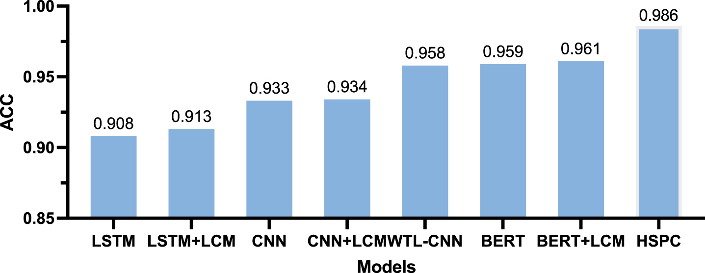
The comparative method in the AGNews dataset is LCM [31] and WTL-CNN [32] which serves as an enhancement component for CNN and LSTM classification models. The comparison of classification accuracy on this dataset for various models is shown in Fig. 4.
The LCM model is a technique used in machine learning to calculate the similarity between samples and labels during training. It generates a label confusion matrix that reduces the impact of label semantic overlap. Inspired by LCM, HSPC introduces an advanced PD correction algorithm to further adjust the label predictions, which also alleviates the impact of label overlap on classification. One problem with LCM is that LCM treats the news text as a whole and does not consider the importance of news titles when it comes to classifying news labels. In contrast, HSPC divides the semantic hierarchy of news texts, which enhances the influence of news titles on news label classification, and thus improves the model’s classification performance on news texts. In terms of accuracy, HSPC outperforms the BERT+LCM model by 2.55Although WTL-CNN extracts both local and global semantic information, it still lacks data enhancement and highly confusing label correction, and the accuracy of HSPC is improved by 2.8% compared with WTL-CNN.
Next, the reasons why the model performs well on the THUCNews dataset are analyzed. It is found that there is a strong correlation between multiple news titles and news labels in the THUCNews dataset. Some titles directly contain words strongly associated with the labels. By considering the title features separately, the model can fully utilize the most relevant label information in the titles and has a significant improvement in accuracy.
Fig. 4
Classification ACC performance comparison chart for THUCNews dataset.
3.3.4Comparison of classification performance for Ohsumed oriented datasets
The main comparative method in the Ohsumed dataset is BERTGCN [33], HyperGAT [34] and Text-level-GCN [35]. Figure 5 shows the accuracy comparison results of various models.
Fig. 5
Classification ACC performance comparison chart for Ohsumed dataset.
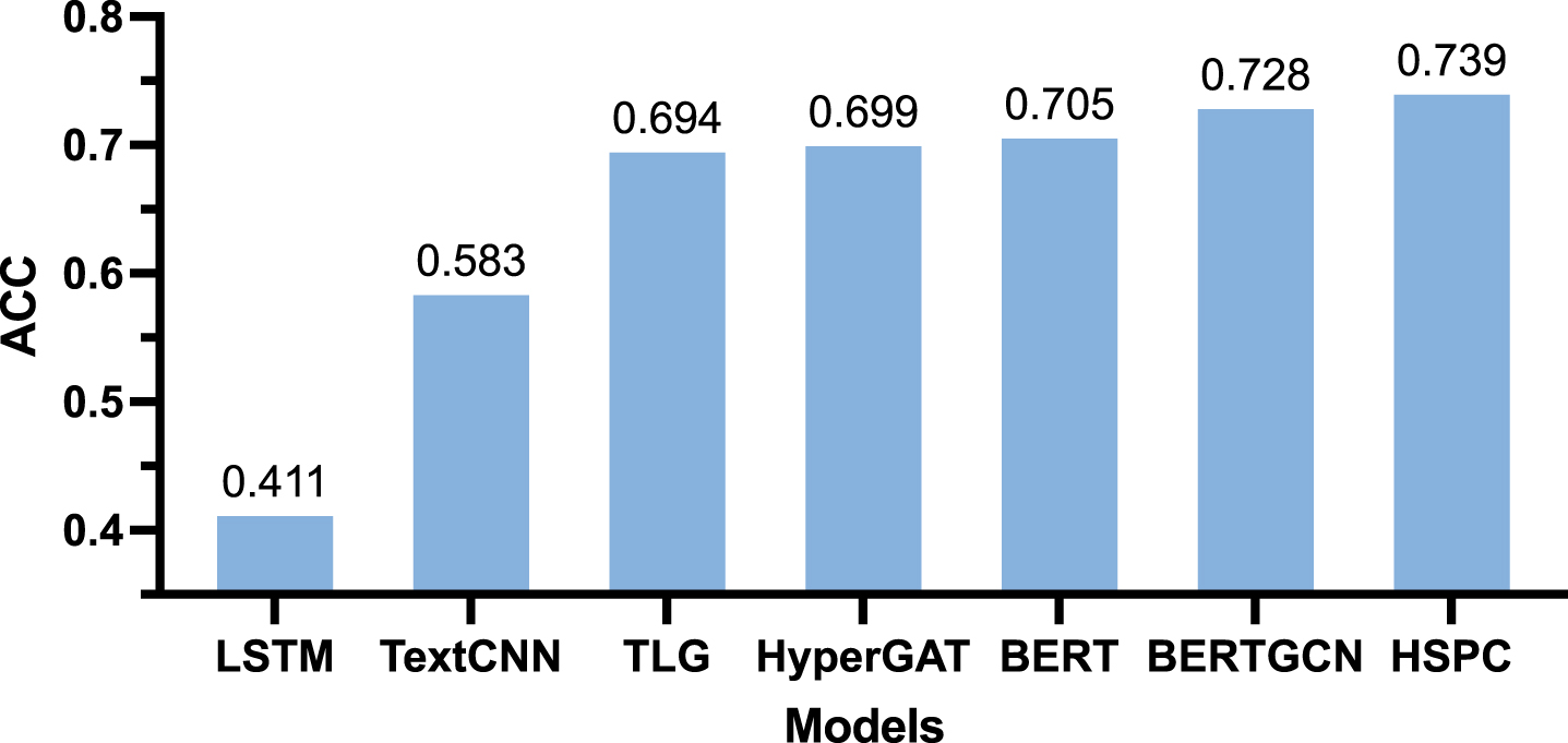
There is still room for improvement in BERTGCN in some aspects. On one hand, the adjacency matrix constructed by BERTGCN for node information exchange remains unchanged during model training, which means the model cannot dynamically focus on strongly related label information in the text. On the other hand, BERTGCN fails to fully consider the differences in the impact of labels and text on label classification, neglecting the influence of titles on news label classification. Similarly, other graph neural networks, whether using Text-level-GNN with document subgraphs or hypergraph neural networks that incorporate topic information, treat news texts as a whole without utilizing the hierarchical semantic features of news texts. Additionally, all other models did not consider highly confusing predictions in label prediction.
Therefore, HSPC, which focuses on hierarchical semantics and performs label prediction correction, exhibits better classification performance on the Ohsumed dataset. It surpasses the BERTGCN model by 1.15% in terms of classification accuracy.
3.4Ablation experiment
The ablation experiment design of HSPC consists of two aspects: hierarchical ablation comparison and training ablation comparison. To make the experimental results clearer, the ablation experiments do not use the PD correction algorithm to adjust the label prediction outputs in the performance testing of all datasets.
3.4.1Hierarchical ablation comparison
To validate the rationality of hierarchical analysis and the necessity of the gate mechanism, the following ablation experiments are conducted.
Reduce title: This approach adopts the idea of extracting overall features without analyzing the hierarchical semantic characteristics of the news text.
Average: This approach uses the hierarchical analysis method but does not consider the fusion method between the title and the body text.
Hierarchical Semantics news text classification model: This approach adopts the hierarchical analysis method and uses the gate fusion mechanism to combine the title features and the full-text features of the news.
The comparative metrics are accuracy and F1 score. The ablation comparison results in each dataset are shown in Table 4. It can be observed that the Average model achieves better results. On all four datasets, there are improvements in both accuracy and F1 score. The accuracy increases by 1.17%, 1.48%, 1.46%, and 0.84% respectively, while the F1 score increases by 1.30%, 1.56%, 1.37%, and 0.86% respectively. This is because the Average model considers the hierarchical semantics of the labels. Compared to the Reduce title model that adopts overall feature extraction, the Average model shows a significant improvement in accuracy.
Next, the Average model and the HS model are compared. The main difference between them is that HS utilizes the gate fusion mechanism, while Average uses the method of average summation. On the four datasets, compared to the Average, the HS model improves the classification accuracy by 0.15%, 0.24%, 0.07%, and 0.31%, and the F1 score by 0.19%, 0.24%, 0.05%, and 0.37% respectively. It is observed that the HS model performs better on the Ohsumed dataset. This is because the Ohsumed dataset has a significant difference in semantics between the title and the body text, requiring a more balanced consideration of news text samples. The gate fusion mechanism can better balance the semantic relationship between the title and the labels, enabling the framework to focus more on the relevant semantic hierarchy for label classification. Therefore, the HS model with gate fusion performs more prominently on the Ohsumed dataset.
Table 4
Results of hierarchical ablation comparison experiments
| Models | FCT | AGNews | ||
| ACC(%) | F1(%) | ACC(%) | F1(%) | |
| Reduce title | 93.89 | 83.08 | 93.48 | 93.4 |
| Average | 95.06 | 84.38 | 94.96 | 94.96 |
| HS | 95.21 | 84.57 | 95.2 | 95.2 |
| Models | THUCNews | Ohsumed | ||
| ACC(%) | F1(%) | ACC(%) | F1(%) | |
| Reduce title | 97.07 | 97.02 | 72.65 | 61.59 |
| Average | 98.53 | 98.39 | 73.49 | 62.45 |
| HS | 98.6 | 98.44 | 73.8 | 62.82 |
3.4.2Training ablation comparison
To compare the optimization effects of data augmentation and adversarial learning on the Hierarchical Semantics (HS) news text classification model, the following training ablation comparison experiments were designed in this section:
None: No optimization is performed on HS at both the data level and the training level.
+DA: Data augmentation is used to optimize the model training on HS, excluding adversarial learning.
+ADV: Adversarial learning is used to optimize the model training on HS, excluding data augmentation.
ALL: Both data augmentation and adversarial learning are used to optimize the model training on HS.
The comparative metrics are accuracy and F1 score on each dataset. The ablation results on the various datasets are shown in Table 5.
Table 5
Comparison results of data augmentation and adversarial learning ablation
| Models | FCT | AGNews | ||
| ACC(%) | F1(%) | ACC(%) | F1(%) | |
| None | 94.59 | 84.05 | 94.75 | 94.74 |
| +DA | 94.72 | 84.17 | 94.84 | 94.82 |
| +ADV | 95.02 | 84.31 | 95.14 | 95.09 |
| All | 95.21 | 84.57 | 95.2 | 95.2 |
| Models | THUCNews | Ohsumed | ||
| ACC(%) | F1(%) | ACC(%) | F1(%) | |
| None | 98.17 | 97.96 | 73.19 | 62.25 |
| +DA | 98.25 | 98.03 | 73.45 | 62.42 |
| +ADV | 98.4 | 98.07 | 73.71 | 62.57 |
| All | 98.6 | 98.44 | 73.8 | 62.82 |
According to the results shown in the 5, the ALL approach achieves the best results. Compared to the None approach which does not utilize data optimization or training optimization, the ALL approach shows improvements in the accuracy by 0.62%, 0.45%, 0.43%, and 0.61% respectively, while the F1 score increases by 0.52%, 0.46%, 0.48%, and 0.57% respectively on the FCT, AGNews, THUCNews, and Ohsumed datasets.
Overall, adversarial learning demonstrates better optimization effects on the model compared to data augmentation across the four datasets. Both data augmentation and adversarial learning can be seen as adding perturbations to the model’s input while controlling the magnitude of the perturbations to ensure that the transformed samples are similar to the original samples in the semantic space. However, there are two key differences between the two methods. Firstly, the directions and magnitudes of the perturbations added by data augmentation and adversarial learning are different. Secondly, data augmentation optimizes the quality of the dataset outside the model by increasing its diversity to enhance the model’s training effectiveness. Adversarial learning optimizes the model internally by adding perturbations in the direction of gradient ascent to enhance the intensity of model training. Therefore, there is no conflict between the two, and the best effect is achieved when using both at the same time. From the analysis of the results, it can be observed that adding only adversarial learning leads to an improvement in accuracy ranging from 0.1% to 0.3% compared to adding only data augmentation. This is because data augmentation has some external technical dependencies. The quality of translation-based data augmentation relies on the performance of translation software, and the effectiveness of synonym replacement data augmentation depends on the quality of the word vector table. On the other hand, adversarial learning, whether it is the direction or magnitude of the added perturbations, is related to the model itself. It is a training strategy specifically designed for the model. Therefore, in most cases, adversarial learning tends to be more effective.
In terms of the comparative analysis of the enhanced results on different datasets, on the FCT and Ohsumed datasets where label imbalance exists, compared to the None approach without any training or data optimization, the +DA approach with data augmentation improves the accuracy by 0.13% and 0.26% respectively, and the F1 score by 0.12% and 0.17% respectively. On the AGNews and THUCNews datasets with more balanced labels, the accuracy improves by 0.09% and 0.08% respectively, and the F1 score improves by 0.08% and 0.07% respectively. This indicates that data augmentation performs relatively better on datasets with label imbalance.
The comparison of training set sizes before and after data augmentation on the FCT, Ohsumed, THUCNews, and AGNews datasets is shown in Table 6. In the case of the AGNews and THUCNews datasets where label imbalance is not an issue, data augmentation is used to increase the size of the training set by doubling the number of training samples, thereby enriching the semantic diversity of the original data. On the Ohsumed and FCT datasets, data augmentation not only enriches the semantic content of the dataset but also mitigates the label imbalance issue in the dataset. Therefore, the optimization effect of data augmentation is better on the FCT and Ohsumed datasets.
Table 6
Comparison table of model classification accuracy indicators before and after correction
| Datasets | Pre-enhancement | Post-enhancement | Number of | Enhancemen |
| scale | scale | labels | methods | |
| AGNews | 120 000 | 240 000 | 4 | All category enhancements |
| THUCNews | 27 300 | 57 600 | 13 | All category enhancements |
| FCT | 9 804 | 12 134 | 20 | Low frequency category enhancement |
| Ohsumed | 3 357 | 4 377 | 23 | Low frequency category enhancement |
3.5Calibration analysis experiments
This experiment is designed to analyze the changes in sample confusion during the model training process and evaluate the effectiveness of the calibration algorithm. The experimental data analyzed in the results are obtained from a hierarchical model that incorporates adversarial learning. For ease of analysis, Sclear is used to represent the proportion of low confusing samples, Sconfused is used to represent the proportion of highly confusing samples, Pclear is used to represent the accuracy in the low confusing interval, and Pconfused is used to represent the accuracy in the highly confusing interval. The overall accuracy of the model is calculated as follows:
(29)
To better demonstrate the correction effect of the PD calibration algorithm at each stage of model training, the correction effect of the PD correction algorithm is analyzed in detail in terms of the overall correction effect, the proportion and accuracy trends of low confusing samples, and the proportion trend of highly confusing samples.
3.5.1Overall correction effect analysis
To analyze the calibration results of the PD algorithm, the data before and after calibration on different datasets are recorded as shown in Table 7.
Table 7
Comparison table of model classification accuracy indicators before and after correction
| datasets | Accuracy before | Accuracy after | Number | Accuracy |
| correction(%) | correction(%) | of labels | improvement(%) | |
| AGNews | 95.2 | 95.21 | 4 | 0.01 |
| THUCNews | 98.6 | 98.62 | 13 | 0.02 |
| FCT | 95.21 | 95.26 | 20 | 0.05 |
| Ohsumed | 73.8 | 73.95 | 23 | 0.15 |
Based on the data in table 7, it can be observed that the calibration algorithm has a certain corrective effect on the data from each dataset. The calibration effect is more significant on the FCT and Ohsumed datasets, with an improvement of 0.05% and 0.15% in predicted accuracy, respectively. The improvement is relatively modest on the AGNews and THUCNews datasets, with only 0.01% and 0.02% improvement, respectively. This indicates that the PD calibration algorithm can optimize the output probability distribution of the model and improve the classification accuracy.
Comparing the calibration performance of the PD algorithm on each dataset, it is evident that the improvement effect of the PD calibration algorithm is more pronounced on the FCT and Ohsumed datasets compared to the AGNews and THUCNews datasets. This suggests that the PD calibration algorithm performs better in correcting models on datasets with a larger number of labels compared to datasets with fewer labels.
Based on the analysis of the above observations, it can be speculated that the accuracy of low confusing samples and the proportion of highly confusing samples are the main factors influencing the calibration effect of the calibration algorithm. On one hand, as the number of labels increases, the classification difficulty of the dataset also increases, and the number of highly confusing label predictions to be handled also increases. Consequently, the calibration algorithm can better demonstrate its efficacy. On the other hand, the higher the accuracy of low confusing samples, the more reliable their probability distribution, making them a better baseline for correcting predictions of highly confusing samples.
To analyze the role of interval selection in the calibration algorithm and validate the correctness of the category filtering idea, the number of instances where the calibrated algorithm decreased the accuracy is recorded after 50 stable model training iterations. The number of calibration errors with and without interval selection is shown in Table 8. It can be observed that in the 50 instances of calibration after training, the calibration algorithm without interval selection has 3 errors in the FCT dataset, 1 error in the AGNews dataset, 0 errors in the THUCNews dataset, and 8 errors in the Ohsumed dataset. After adding interval selection, the number of calibration errors in the four datasets is reduced to 1 error, 0 errors, 0 errors, and 2 errors, respectively. Compared to the calibration algorithm without interval selection, the addition of interval selection resulted in a reduction of 2 errors, 1 error, 0 errors, and 6 errors in the respective datasets. The stability improvement is particularly evident in the Ohsumed dataset, while the calibration stability does not change significantly in the other three datasets. This occurrence may be because the stability of the calibration algorithm’s correction effect is influenced by the magnitudes of Pclear and Pconfused in the dataset. The higher the values of Pclear and Pconfused in the dataset, the better the stability of the correction.
Table 8
Comparison of fifty correction errors
| Calibration algorithm | FCT | AGNews | ||
| Number of | Error | Number of | Error | |
| errors(times) | rates(%) | errors(times) | rates(%) | |
| No interval filtering | 3 | 6 | 1 | 2 |
| With interval filtering | 1 | 2 | 0 | 0 |
| Calibration algorithm | THUCNews | Obsumed | ||
| Number of | Error | Number of | Error | |
| errors(times) | rates(%) | errors(times) | rates(%) | |
| No interval filtering | 0 | 0 | 8 | 16 |
| With interval filtering | 0 | 0 | 2 | 4 |
3.5.2Analysis of low confusing samples
Low confusing samples serve as a reference for correcting highly confusing samples in the calibration algorithm. Analyzing the accuracy and proportion of low confusing samples can provide better insights into the correction effect of the calibration algorithm. The accuracy and proportion of low confusing samples are recorded during the model training process on the four datasets, and their trend changes are plotted in a line graph as shown in Fig. 6.
Fig. 6
Plot of low confusing sample share and ACC with model training.
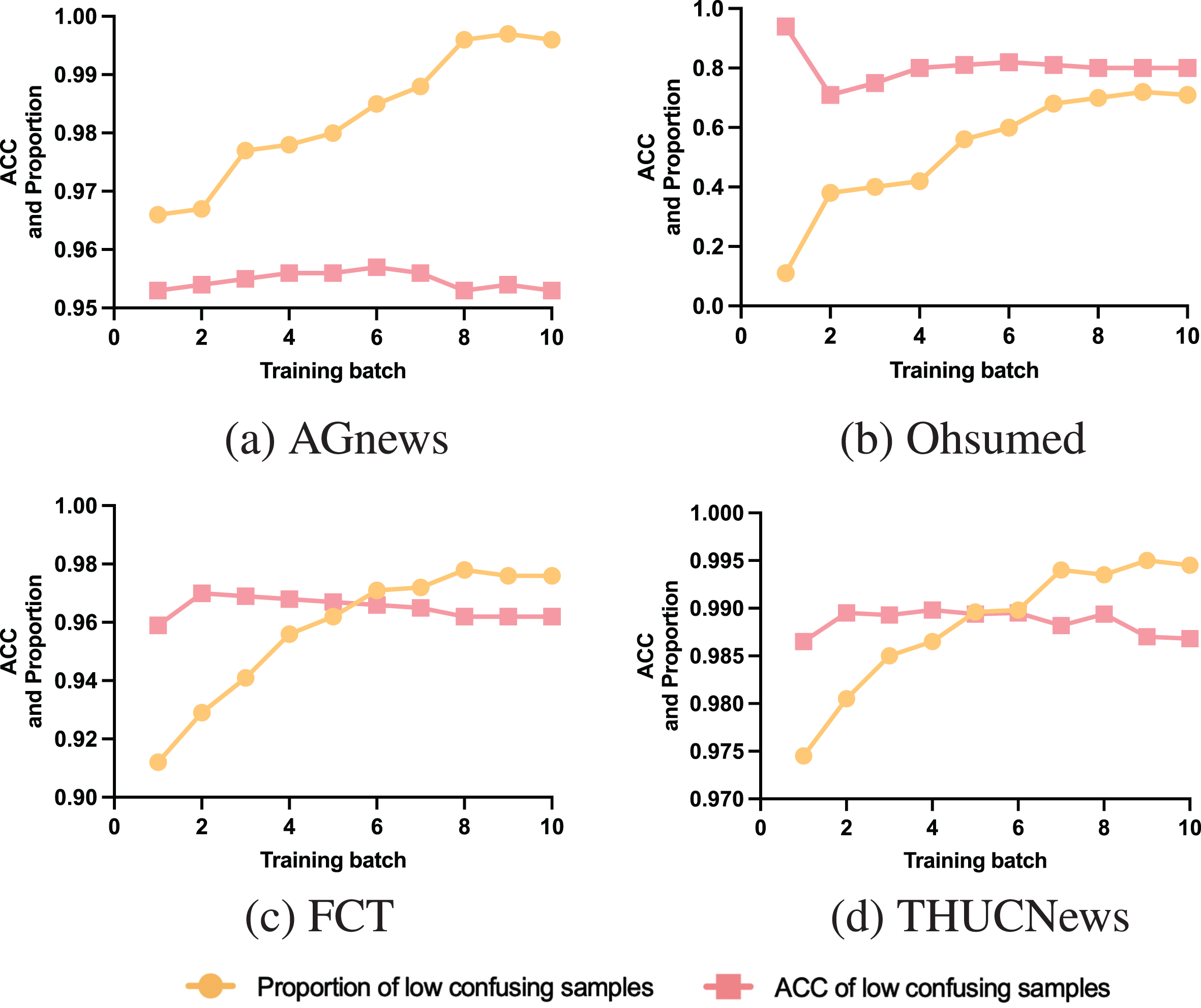
Comparing the accuracy and proportion of low confusing samples in the AGNews and THUCNews datasets, after the model training stabilizes, the Sclear values in both datasets are similar, around 99.5%. However, the difference lies in the Pclear values, where the THUCNews dataset has a higher Pclear, approximately 3.75% higher than that of the AGNews dataset. Therefore, the main factor affecting the correction effect of the PD algorithm on these two datasets is Pclear. The PD algorithm performs better in correcting the THUCNews dataset compared to the AGNews dataset. Comparing the FCT dataset and the AGNews dataset, the increase in Pclear in the FCT dataset is not significant, around 1.0%. However, compared to the Sclear of approximately 99.5% in the AGNews dataset, the proportion of Sclear in the FCT dataset is around 97.5%, meaning that Sconfused in FCT is 2.5%, which is six times that of the AGNews dataset. Therefore, in the FCT and AGNews datasets, the influence of Sclear on the correction algorithm is more significant, and the PD algorithm performs better in the FCT dataset.
This comparative analysis confirms the speculations made in the contrast analysis of the calibration effect. Firstly, when the accuracy of low confusing samples is similar, the larger the proportion of highly confusing samples, the better the correction effect. Secondly, when the proportion of highly confusing samples is approximately the same, the higher the accuracy of low confusing samples, the better the correction effect.
3.5.3Analysis of highly confusing samples
highly confusing samples are the main focus of the PD algorithm’s correction. Analyzing the accuracy and proportion of highly confusing samples can provide a better understanding of the correction effect of the calibration algorithm. The variation trends of the proportion and accuracy of highly confusing samples are shown in Fig. 7.
Fig. 7
Plot of highly confusing sample share and ACC with model training.
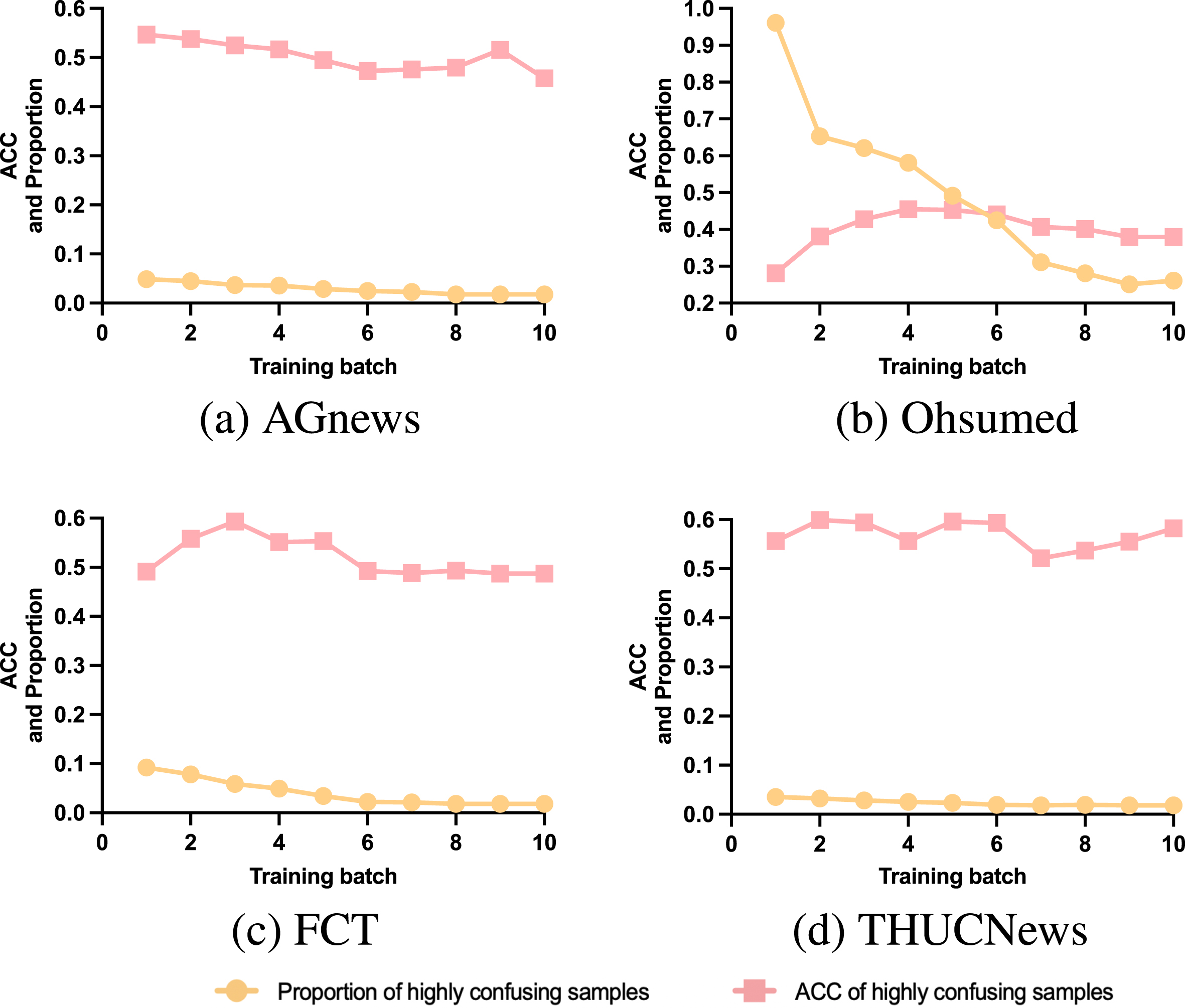
Comparing the four subgraphs (a), (b), (c), and (d), except for the Ohsumed dataset, where Pconfused is approximately 40%, the Pconfused values in the other three datasets are around 50%. However, the Sconfused values in the other datasets range from 0.5% to 2.0%, while the Sconfused value in the Ohsumed dataset is approximately 22.0%, significantly higher than the other datasets. Therefore, even though the Ohsumed dataset has lower values of Pclear and Pconfused compared to the other three datasets, its higher proportion of Sconfused allows for more samples to be corrected by the PD algorithm. Overall, the PD algorithm performs the best on the Ohsumed dataset.
The Ohsumed dataset has lower values of Pclear and Pconfused compared to the other datasets, indicating that the correction effect in this dataset exhibits instability, confirming the speculation made in the calibration stability analysis. However, due to the presence of an interval selection algorithm, which eliminates most of the unlikely options, the negative impact caused by the low values of Pclear and Pconfused in the Ohsumed dataset is alleviated. This improves the stability of the correction and ensures the effectiveness of label prediction.
4Conclusion
This paper proposes a news text classification framework HSPC. Firstly, the dataset is optimized using data enhancement to increase sample richness. To improve the model’s robustness, adversarial is added. During feature extraction, a hierarchical approach is used with a gate fusion mechanism. A pre-trained model is then applied to extract contextualized features for downstream classification. During the prediction phase of the news text classification framework, entropy is utilized as a metric to calculate confusion, which helps to identify highly confusing labels accurately. Additionally, a prior distribution is used for targeted correction, which results in an improved classification accuracy.
The experiment utilized four datasets, two in Chinese and two in English, to thoroughly compare and analyze the classification performance of HSPC with other models for news text classification. The results demonstrated the effectiveness of the hierarchical analysis approach. By conducting ablation experiments, the study verified the efficacy of the gate mechanism, data augmentation, and adversarial learning in enhancing classification prediction. Moreover, the calibration analysis experiment comprehensively examined the accuracy changes of highly confusing samples, low confusing samples, and the overall correction effect, confirming the suitability of the calibration algorithm design.
In the future, more advanced adversarial learning approaches and data augmentation techniques will be conducted in HSPC for news text classification. Additionally, while HSPC currently uses only text data, future work aims to integrate multi-modal data such as images and videos for comprehensive analysis of news content.
Acknowledgment
This research is supported by the National Natural Science Foundation of China (Grant No. 62272180), Research Topic of Hubei Vocational and Technical Education Association, “Research on Application of Building Vocational Education Regional Data Center to Promote Industrial Development and Supply-Demand Linkage” (ZJGA2023014), University-level Scientific Research Startup Fund Project, “Key Technology Research on Big Data and AI Middle Office” (KYQDJF2023004), Philosophy and Social Science Research Project of Hubei Provincial Department of Education (No. 21D111) and Wuhan Vocational College of Software and Engineering 2023 Doctor Team Science and Technology Innovation Platform Project (No. BSPT2023001).
References
[1] | Chen J. , Gong Z. and Liu W. , A Dirichlet process term-based mixture model for short text stream clustering, Appl Intell 50: ((2020) ), 1609–1619. |
[2] | Li R. , Chen H. , Feng F. , Ma Z. , Wang X. , Hovy E. Dual Graph Convolutional Networks for Aspect-based Sentiment Analysis, in: Proceedings of the 59th Annual Meeting of the Association for Computational Linguistics and the 11th International Joint Conference on Natural Language Processing (Volume 1: Long Papers), Association for Computational Linguistics, Online, 2021, 6319–6329. |
[3] | Qurashi A.W. , Holmes V. , Johnson A.P. Document Processing: Methods for Semantic Text Similarity Analysis, in: 2020 International Conference on INnovations in Intelligent SysTems and Applications (INISTA), IEEE, Novi Sad, Serbia, 2020, 1–6. |
[4] | Zheng M. , Jiang K. , Xu R. and Qi L. , An adaptive LDA optimal topic number selection method in news topic identification, IEEE Access 11: ((2023) ), 92273–92284. |
[5] | Wu C. , Wu F. , Huang Y. and Xie X. , Personalized news recommendation: methods and challenges, ACM Trans Inf Syst 41: ((2023) ), 1–50. |
[6] | Hnaif A.A. , Kanan E. and Kanan T. , Sentiment Analysis for Arabic Social Media News Polarity, Intelligent Automation & Soft Computing 28: ((2021) ), 107–119. |
[7] | Zhang M.-L. and Zhou Z.-H. , ML-KNN: A lazy learning approach to multi-label learning, Pattern Recognition 40: ((2007) ), 2038–2048. |
[8] | Tan S. , Neighbor-weighted K-nearest neighbor for unbalanced text corpus, Expert Systems with Applications 28: ((2005) ), 667–671. |
[9] | Nédellec C. , Rouveirol C. eds., Machine learning: ECML-98: 10th European Conference on Machine Learning, Chemnitz, Germany, April 21–23, 1998: proceedings, Springer, Berlin; New York, 1998. |
[10] | Peng T. , Zuo W. and He F. , SVM based adaptive learning method for text classification from positive and unlabeled documents, Knowl Inf Syst 16: ((2008) ), 281–301. |
[11] | Goudjil M. , Koudil M. , Bedda M. and Ghoggali N. , A novel active learning method using SVM for text classification, Int J Autom Comput 15: ((2018) ), 290–298. |
[12] | Agduk S. , Aydemi E.R and Polat A. , Classification of news texts from different languages with machine learning algorithms, Journal of Soft Computing and Artificial Intelligence 4: ((2023) ), 29–37. |
[13] | Ramkissoon A.N. and Goodridge W. , Enhancing the predictive performance of credibility-based fake news detection using ensemble learning, Rev Socionetwork Strat 16: ((2022) ), 259–289. |
[14] | Bafna P. , Saini J.R. Hindi poetry classification using eager supervised machine learning algorithms, in: 2020 International Conference on Emerging Smart Computing and Informatics (ESCI), IEEE, Pune, India, 2020, 175–178. |
[15] | Dogra V. , Verma S. , Verma K. , Jhanjhi N. , Ghosh U. and Le D.-N. , A comparative analysis of machine learning models for banking news extraction by multiclass classification with imbalanced datasets of financial news: challenges and solutions, IJIMAI 7: ((2022) ), 35. |
[16] | Deng L. , Ge Q. , Zhang J. , Li Z. , Yu Z. , Yin T. and Zhu H. , News text classification method based on the GRU_CNN model, International Transactions on Electrical Energy Systems 2022: ((2022) ), 1–11. |
[17] | Wu H. , Li D. and Cheng M. , Chinese text classification based on character-level CNN and SVM, IJIIDS 12: ((2019) ), 212. |
[18] | Nguyen H. , Nguyen M.-L. A deep neural architecture for sentence-level sentiment classification in twitter social networking, in: K. Hasida and W.P. Pa (Eds.), Computational Linguistics, Springer Singapore, Singapore, 2018, 15–27. |
[19] | Chen Z. , Qian T. Transfer capsule network for aspect level sentiment classification, in: Proceedings of the 57th Annual Meeting of the Association for Computational Linguistics, Association for Computational Linguistics, Florence, Italy, 2019, 547–556. |
[20] | Zhang Y. , Yu X. , Cui Z. , Wu S. , Wen Z. , Wang L. Every document owns its structure: Inductive text classification via graph neural networks, in: Proceedings of the 58th Annual Meeting of the Association for Computational Linguistics, Association for Computational Linguistics, Online, 2020, 334–339. |
[21] | Liu L. and Sun Y. , Research on topic fusion graph convolution network news text classification algorithm, International Journal of Advanced Network, Monitoring and Controls 7: ((2022) ), 90–100. |
[22] | Sun Y. , Wang S. , Li Y. , Feng S. , Chen X. , Zhang H. , Tian X. , Zhu D. , Tian H. , Wu H. ERNIE: Enhanced Representation through Knowledge Integration, (2019). |
[23] | Liu Y. , Ott M. , Goyal N. , Du J. , Joshi M. , Chen D. , Levy O. , Lewis M. , Zettlemoyer L. , Stoyanov V. RoBERTa: A Robustly Optimized BERT Pretraining Approach, (2019). |
[24] | Devlin J. , Chang M.-W. , Lee K. , Toutanova K. BERT: Pre-training of Deep Bidirectional Transformers for Language Understanding, (2018). |
[25] | Garg S. , Ramakrishnan G. BAE: BERT-based Adversarial Examples for Text Classification, in: Proceedings of the 2020 Conference on Empirical Methods in Natural Language Processing (EMNLP), Association for Computational Linguistics, Online, 2020, 6174–6181. |
[26] | Kim Y. Convolutional Neural Networks for Sentence Classification, in: Proceedings of the 2014 Conference on Empirical Methods in Natural Language Processing (EMNLP), Association for Computational Linguistics, Doha, Qatar, 2014, 1746–1751. |
[27] | Graves A. Generating Sequences With Recurrent Neural Networks, (2013). |
[28] | Lyu S. and Liu J. , Convolutional recurrent neural networks for text classification, Journal of Database Management 32: ((2021) ), 65–82. |
[29] | Tao H. , Tong S. , Zhang K. , Xu T. , Liu Q. , Chen E. and Hou M. , Ideography leads us to the field of cognition: A radical-guided associative model for chinese text classification, AAAI 35: ((2021) ), 13898–13906. |
[30] | Li X. , Li Z. , Xie H. and Li Q. , Merging statistical feature via adaptive gate for improved text classification, AAAI 35: ((2021) ), 13288–13296. |
[31] | Guo B. , Han S. , Han X. , Huang H. and Lu T. , Label confusion learning to enhance text classification models, AAAI 35: ((2021) ), 12929–12936. |
[32] | Zhao W. , Zhu L. , Wang M. , Zhang X. and Zhang J. , WTL-CNN: a news text classification method of convolutional neural network based on weighted word embedding, Connection Science 34: ((2022) ), 2291–2312. doi:10.1080/09540091.2022.2117274. |
[33] | Lin Y. , Meng Y. , Sun X. , Han Q. , Kuang K. , Li J. , Wu F. BertGCN: Transductive Text Classification by Combining GNN and BERT, in: Findings of the Association for Computational Linguistics: ACL-IJCNLP 2021, Association for Computational Linguistics, Online, 2021, 1456–1462. |
[34] | Ding K. , Wang J. , Li J. , Li D. , Liu H. Be More with Less: Hypergraph Attention Networks for Inductive Text Classification, in: Proceedings of the 2020 Conference on Empirical Methods in Natural Language Processing (EMNLP), Association for Computational Linguistics, Online, 2020, 4927–4936. |
[35] | Huang L. , Ma D. , Li S. , Zhang X. , Wang H. Text Level Graph Neural Network for Text Classification, in: Proceedings of the 2019 Conference on Empirical Methods in Natural Language Processing and the 9th International Joint Conference on Natural Language Processing (EMNLP-IJCNLP), Association for Computational Linguistics, Hong Kong, China, 2019, 3442–3448. |


