
Financial derivative features based integrated potential fishing zone (IPFZ) Future forecast
Abstract
In India, around 7 million people depend on fishing for their livelihoods. They are assisted with a reliable and fast brief forecast for the areas of fish aggregations. Habitat mapping is critical in supporting strategic choices on fish usage and protection. In conjunction with techniques for machine learning, remote control has made comprehensive fish mapping on relevant scales possible. In machine learning, supervised algorithms are utilized to make forecasts from datasets, when data is accessible without relating output factors. In this research work, Ocean Surface Temperature (OST) and Satellite derived Chlorophyl material are the basic inputs to generating the information of Potential Fishing Zone (PFZ). The 16 features and additional financial derivative features are used for accurate future prediction of PFZ. The unwanted and missing data are removed using effective pre-processing techniques. Among the various methods available for forecasting nonlinear phenomena, the Neural Network is the best and the efficient method to get a forecast. Therefore, the Function Fitting Neural Network (FFNN) technique is mainly used to predicting the Integrated Potential Fishing Zone (IPFZ). The practical analyses are performed by analysing the 80% -20%, 60% -40% and future data in terms of various parameters. From the results, it is proved that the suggested FFNN achieved 90% of accuracy, where the existing neural network achieved 86% of accuracy by implementing with financial derivative features for the 80% -20% of available dataset.
1Introduction
Fishery development is subject on availability of natural resources, appropriate funding, adequate novel technology, fishing unit growth, fishing extension, government policies, Morden technologies, and grassroots technical information. In terms of the makeup and dynamics of its species, the marine environment is complicated. With the rises in fishing fleets, the traditionally known fishing grounds are under enormous pressure and fishing per unit effort (CPUE) decline [1] per unit effort. Through remote sensing techniques, it is therefore necessary to distract some fishing efforts from other relevant potentially fishing regions. The prediction of structures and functions in the marine eco system requires on an in-depth appreciative of the physical and natural process that regulates organisms’ great quantity distribution and output and a wide diversity of time and wide diversity of time space levels [2].
In order to study chlorophy’s link to sea surface temperature with employed Coast Zone Colour Scanner (CZCS) and (OST) [3]. The water mass classification seems to be linked to various biological and physical processes. In 1989-90, the prediction for Potential Fishing Zones (PFZs), with NOAA AVHRR OST computed in India, was launched [4] With the emergence and quick spread of satellite remote sensing that leads to the deployment of remote sensors for specific parameters, OST, CHL and PAR data collected from satellites are available as Global Area Coverage (GAC) for the previous two decades [5]. In this context it has become an important data source to explain the linkages between exploited marine animals and their habitat for the availability of world, daily, systemic images taken from satellites. To examine the distribution, abundance and migratory of fishes, continual archiving of remotely sensed satellite parameters in a particular region is necessary. Remote sensing has played an essential role in marine fisheries management and use since 1978. Neural network approaches are used [6, 7] to anticipate fishing zones.
Brain networks are simple nonlinear computing components that imitate the neural system of the human being. Brain networks are named between input and output layers as hidden layers and often called neurons [8]. When loading data into the ANN (Artificial Neural Network), it must be pre-processed into the numerical range with which the ANN can handle the efficiency of the learning results efficiently. The advantages of using PFZ advisories to the Indian fishing community were described in this research. A quantitative study of the net profit gains gained by the reduction in the time for the search and better catches and the percentage of success in PFZ-led fishing is presented.
The remains of this document are follows: The associated works for the IPFZ prediction are discussed in Section 2. The recommended methodology employed in this paper was outlined in Section 3. The study concludes with its future work in Section 4 and Section 5 to provide the outcomes and discuss the results.
2Related works
In the most Economic Zone inedible the eastern coastline of Malaysia, MODIS satellite pictures with fishery catch data of 2008 have been generated by [9] in the Rastrelliger Kanagurte PAFZ, Rastrelliger Kanagurta (Cuvier 1817). The photos were classed with appropriate scores and integrated to produce a prospective map using GIS based on the selected ranges. The results showed a preferred CHL range of 0.27±0.030 mg/m3 for the greatest catch and OST of 29.91±0.33 °C. In the mapping of possible fishing grounds, a total accuracy of 75% was attained. This study shows how the Satellite Images and GIS can map R. Kanagurta’s possible fishing areas as well as how the biophysical characteristics are related to fishing data.
In order to discover the relationships among their spatiotemporal distribution and the ecological factors, [10] developed the HSI model to identify possible fishing surroundings for sword fishes in the southern Atlantic with long-water fishery and distance sensing data for the years 1998-2007 in Taiwan. With most CPUE-defined variations explained by OST, all environmental considerations such as OST, assorted layer depth (ALD, SSHA), Ocean surface and height are abnormality and ocean Bathymetric (BAH) were extremely significant. In locations with OST 27–28 C, SSHA -0.05 - 0.05 m, CHLs 0.1-0.2 mgm-3 and BAH 4000 to 4500 m, the most optimal habitat has been found (i.e. hotspot). According to the calculation of numerous pragmatic HSI models in grouping with various ecological conditions, the arithmetical average model with five ecological variables was shown to be most acceptable. The biweekly maps in the projected HSI measurements were checked by the experiential catch per unit effort and suggested that this model may be utilized as a tool to trustworthy forecast for probable fishing grounds.
A short period of time association between skipjack tuna and ocean surface conditions was outlined using fisheries data from [11]. The remote sensing of OST and CHL (MODIS) were used to illustrate the expected high capture zones. The highest skipjack CPUEs were recorded mostly during the 2007 and 2009 study period in the coastal regions of Palopo and Kolaka. The high tuna levels were well equivalent to 0.15-0.40 mg mg3 CHL and 29.0-31.5°C OST. OST was good. The preferred ranges are a good indicator to locate possible fishing sites for skipjacks at first.
With the use of MODIS data on periodic spatial sharing to the Ocean surface salinity (OSS), OST and CHL in sea waters off the coast of Semporna, Malaysia, [12] have shown to be projected by a potential fishery map. The OSS was evaluated with the multi-linear regression analysis and the Brown and Minnet algorithms were employed for the OST. The parameters obtained have been validated by means of in situ Hydro-Lab equipment measurement. The factors are retrieved from adequate resolution imaging spectro-radiometer (MODIS) photos indicate the monogram values establishing the links among these strictures, thus outlining the PFZ map. The Rô was calculated at 0.93, and the larger fish catching areas correlated with the greater PFZ levels, which means the technique are ready to be used for near-real-time fish predictions.
The Developed a Decision Support System to forecast the fishing ground of short Mackerel employing MODIS satellite images [13]. The input data for the development of Potential Fishing Zone is Sea Surface Temperature, CHL and fish catch data with fishing locations. The results displayed that OST and CHL – circulations have a nearby connection to the sharing of the fishing location of the short Mackerel to regulate the association among catcher and oceanographic parameters of linear regression. The range of Sea Surface Temperature from 26 C to 29 C and CHL - a from 1.19 mg/m3 to 1.25 mg/m3 identified as the fishing location for short Mackerel in Makassar strait.
Stimulated by artificial neural network features. This research suggested alternative IPFZ prediction approaches based on the Neural Network. As described below, our key contributions include:
❖ Four models for learning Neural Networks with the ability to accurately predict IPFZ were proposed.
❖ The accuracy of the Better classification was achieved by applying FFNN.
❖ Furthermore, we calculate the characteristics with the compliance of the natural time order of the data instead of selecting variables that ignore the time order.
3Proposed system
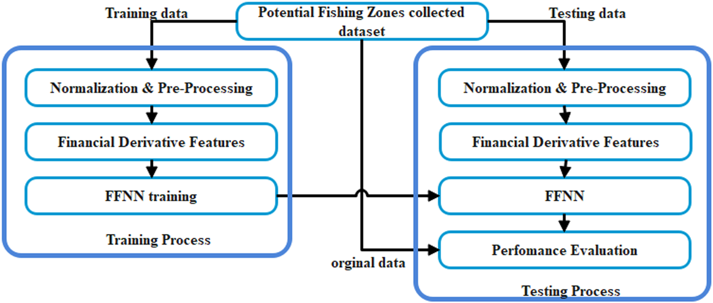
Most of the research articles are not supporting for this Potential Fishing Zones (PFZs) future forecast, so we have referred some of the rainfall detection related articles because of the type of the input raw data’s are maximum related to this work. From that analysis we find [14] which leads improve the number of features information’s based on the Financial Derivatives and geometrical features. This Economic Derivatives features and geometric structures are support the Function Fitting Neural Network to predict the future PFZs accurately. The Architecture of the proposed Financial Derivative Features based IPFZ Future Forecast is shows in the Fig. 1.
Fig. 1
Proposed Financial Derivative Features based IPFZ Future Forecast Architecture.
3.1Dataset
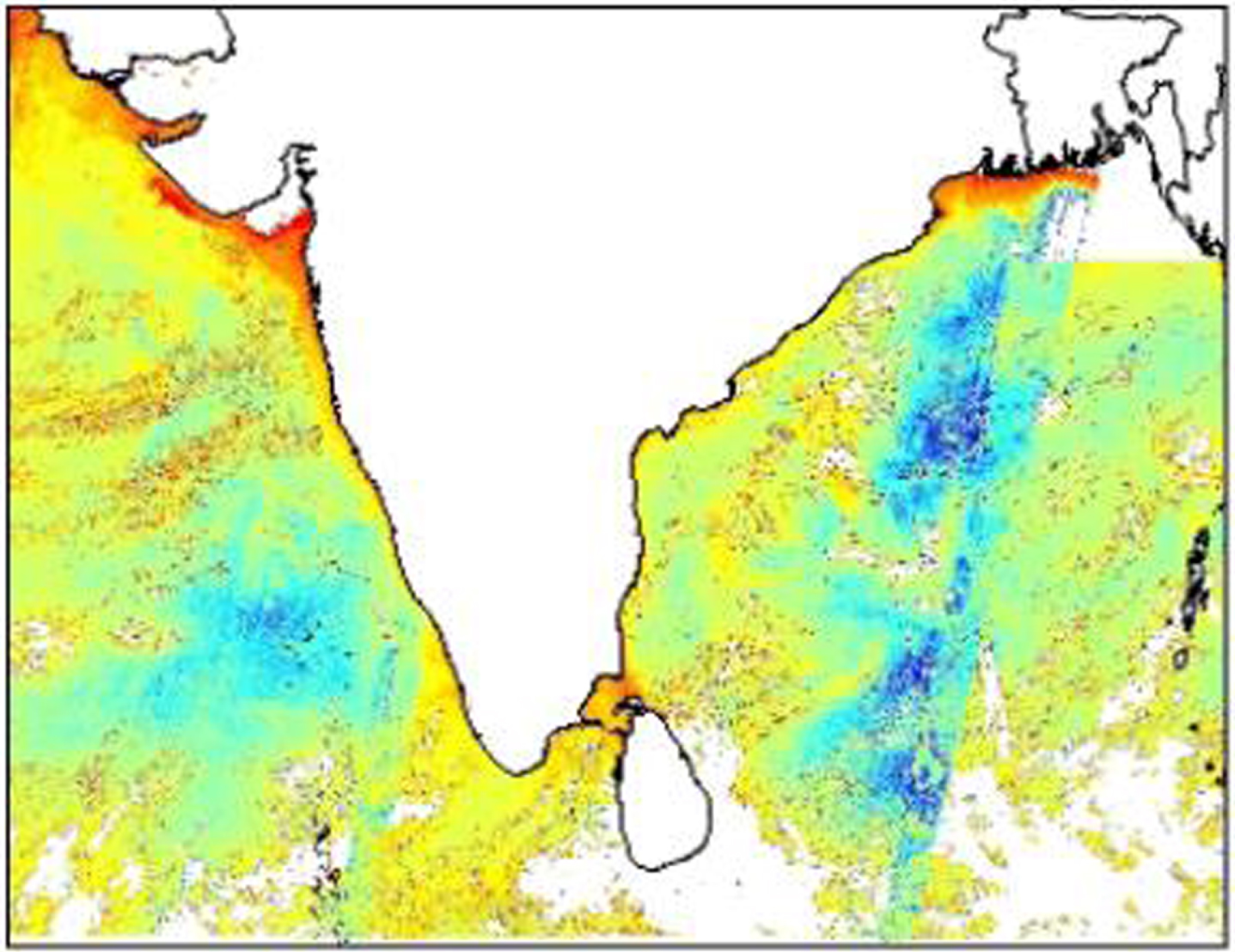
Ocean Surface Temperature data (OSTs), chlorophyll, and Ocean Sat II - India (Fig. 2) Optical Communication Band, and MODIS Aqua (US) are used to detect potential fishing zones all over the place of the Indian coastline, which are regularly together by NOAA-AVHRR thermal-infrared frequencies and Eumetsat (ESA) Met-OP satellites. For each sector PFZ Announcements are produced in the form of PFZ Maps and Texts, and where PFZ are positioned (latitude and longitude data). Because of the sea’s lively atmosphere, the selected place could be progressed by recognised fishing zones on the atlases. The wind speediness and route information is also incorporated into the PFZ maps to guide fisherman on the likely shifts in PFZ. This fact allows the fishermen to trace the PFZ in the maps; on the other hand after a day they will reach the site. The PFZ maps and text for the accessibility of fisherman are also obtained in each sector’s with their local languages. The PFZ text gives data about exact position of (length, latitude), depth at the PFZ site and the distance from important places on the coastlines (fishing landing stage centre, light erections) clearly identifiable.
Fig. 2
Retrieved Oceansat-2 Satellite Data Chlorophyl Image.
3.2Pre-processing & normalization
The unused data and the missing datas are cleaned using pre-processing methods. In addition, the shape of the data are altered during normalization method. In the beginning, the total number of the input uncooked data is around 151031 with 16 features. The whole raw datas are taken as training data and Table 1 describes the total number of features.
Table 1
Feature description
| Number of Features | Description |
| 1 | Landing_Center (LC) |
| 2 | UPDATED_DATE (UD) |
| 3 | DIRECTION (DIR) |
| 4 | ANGLE |
| 5 | DISTANCE_FROM (DIF) |
| 6 | DISTANCE_TO (DIT) |
| 7 | DEPTH_FROM (DEF) |
| 8 | DEPTH_TO (DET) |
| 9 | LONGITUDE_DEGREE |
| 10 | LONGITUDE_MINUTE |
| 11 | LONGITUDE_SECOND |
| 12 | LONGITUDE_DIRECTION |
| 13 | LATITUDE_DEGREE |
| 14 | LATITUDE_MINUTE |
| 15 | LATITUDE_SECOND |
| 16 | LATITUDE_DIRECTION |
Among the 16 features UPDATED_DATE is use as targeted data to training the suggested model. The input information is taken from 15-5-2013 to 18-7-2018, where the main aim of the objective is to predict the potential fishery zone by giving future data. Hence, only 15 unique features are used in this research, however, only 13 unique features are used for training the system. The reason is that the feature LONGITUDE_DIRECTION (East) and LATITUDE_DIRECTION (North) has same information for 151031 data, which is not useful for training the proposed model. In order to training the projected network and attain improved classification precision, the “-“ between the date is removed for the period of pre-processing. The DIRECTION feature has seven directions as Southern East (SE), Southern West (SW), Northern East (NE), Southern (S), East (E), Northern (N) and Western (W). This datas are cannot be use openly to train the projected model, hence these characters are rehabilitated into variable. In addition, the Landing_Center attribute are in an floating format, which is altered into double layout for improved prediction. Hence, 13 features are known as input to the FFNN for predicting the PFZ. Moreover, in order to accurately predict the future PFZ, this research study uses more quantity of features such as Economic Derivatives and geometrical metrics, which is described as follows.
3.3Financial derivative features
The way the dataset are deal with is another deliberation, as it is uncommon for raw data values to be give back to an algorithm to be used. The data should consequently be revised to fit our challenging domain. The aim of this research work is to predict the IPFZ over the well-defined region based on the collected fish capacity. An important factor that needs to be considered is the need to come to an end of future agreements, usually up to one year in advance, and the indenture period might take any length. In addition, given the unique character of the PFZ projections, there is an even higher need for data transformation. Therefore, we employ an Economic Derivative feature (Table 2) to give the data more understandable and more appropriate for the problem area. The result looks to be much less altered, which is why financial derivatives are applied, with adding, volatility on a daily basis appears to be lesser and a pattern is ease to recognize in PFZ predicting. This approach of predicting IPFZ is extremely flexible and may be altered to any length of interest.
Table 2
List of financial derivative and geometrical features used
| S. No | Financial Derivative Features |
| 1 | Autocorrelation |
| 2 | Mean Standard |
| 3 | Contrast |
| 4 | Deviation Sum |
| 5 | Correlation |
| 6 | Difference Adjacent |
| 7 | Cluster Prominence |
| 8 | Difference Moving |
| 9 | Cluster Shade |
| 10 | Average Standard |
| 11 | Dissimilarity |
| 12 | Deviation across MA |
| 13 | Energy |
| 14 | Last Maximum |
| 15 | Entropy |
| 16 | Last Minimum |
| 17 | Homogeneity |
| 18 | Maximum probability |
| 19 | Time Last Maximum |
| 20 | Sum variance |
| 21 | Time Last Minimum |
| 22 | Magnitude of Minimum |
| 23 | Magnitude of Maximum |
| 24 | Minimum Last Contract Length |
| 25 | Maximum Last Contract Length |
| 26 | Modification of Minimum over Last Contract Length |
| 27 | Modification of Maximum over Last Contract Length |
3.4Classification
The more number of features are set as input to the proposed FFNN technique for forecasting the PFZ, where the different types of neural networks are used to validate the presentation of the projected ideal. These neural networks include ENN, RNN and CFN are also discussed as in Comparative Techniques.
3.4.1Proposed Function Fitting Neural Network (FFNN)
A neural network associates a number of levels of processing, engaging basic, simultaneous and biologically nervous-inspired parts. It encompasses of a layer of input, one or numerous hidden layers and a layer of output. In every layer, the input of each layer involves of a number of nodes, or neurons, so that neurons join the different layers. Typically every neuron has weights modified during the learning process and modifies the strength of the signal of this neuron as the weight decreases or grows. The structure of a FFNN is defined in the Fig. 3.
Fig. 3
Single node in a FFNN network.
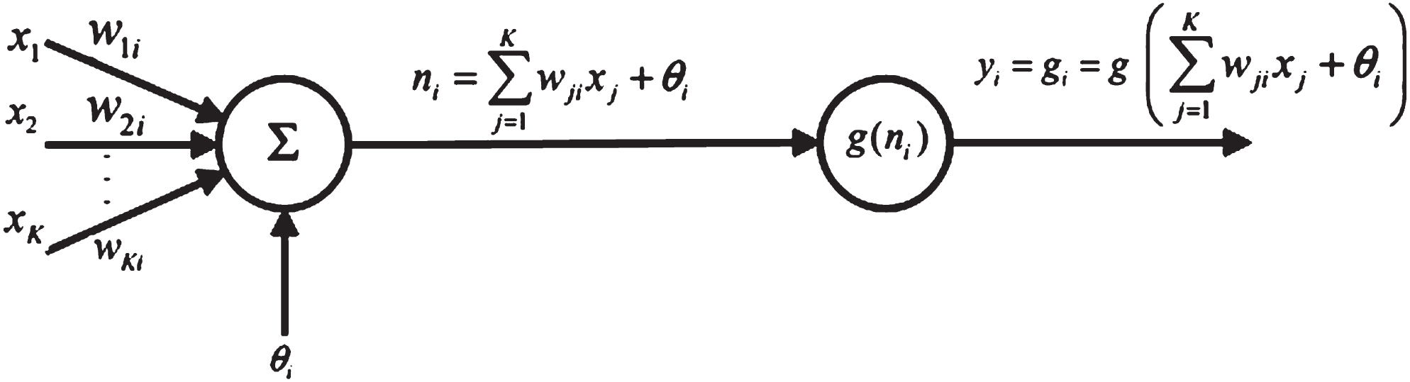
The inputs of the neuron xk, k = 1, … k, and the continuous bias term θi are multiplying and added up. The result of n i shall be the g-enabled input. Initially, however, a hyperbolic tangent (tanh) or a sigmoid function is the most common activation function for the mathematical accessibility. Tangent is defined as hyperbolic
(1)
(2)
Linking many nodes in parallel and series, a FFNN network is intended. A typical network for single hidden layer is shown in Fig. 4.
Fig. 4
FFNN with one hidden layer.
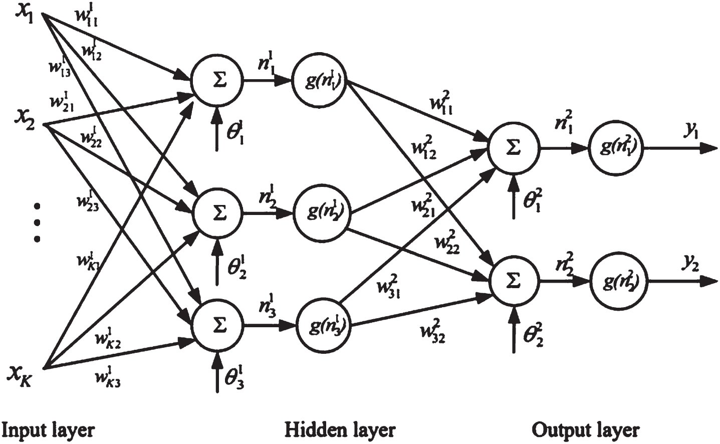
The output, yi i = 1 and 2, of the FFNN network becomes
(3)
From (3) we may deem a non-linear map from the input space x to the output space (m = 3), the FFNn is a non-linear parameterised map (here m = 3). The weights of Wji and biases are parameters of
When you use data (xi, yi) i = 1, … . N, it is a data fitting issue to discover the optimal FFNN network. The parameters
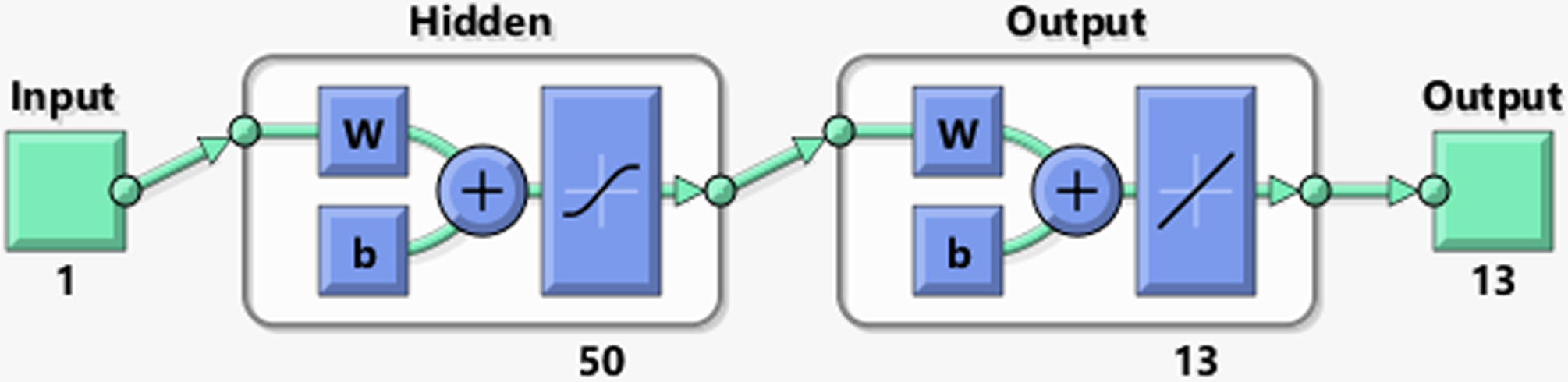
This is the procedure. The designer must first f the architecture of the FFNN network: the number of layers and neurons concealed in each layer. Figure 5 shows the total architecture. At this point, too, the activation functions for each layer are expected to be known. The weights and biases
Fig. 5
The Proposed MATLAB FFNN Architecture.
After procurement the results from FFNN, the post-processing is passed out. In this strategy, the twofold organize of LC include is changed over into characters. The factors of DIR are adjusted into seven directions. Subsequently, the comes about will be in an appropriate arrange, for occasion in case an client allow a future information as input, the location label name, its flow direction, latitude and longitude bearings are shown as yield of FFNN show [15].
3.5Comparison neural network models
3.5.1Elman neural network
A feedback neural system improved by Elman in 1990 can be characterized as the Elman Neural Network (ENN). ENN focuses on the training of the neural background network (BPNN). The Elman neural network architecture is usually divided into 4 layers. The undertaking layer function is to save the output of the cached layer. The output of the hidden layer connections its entrance through the delay and the storage of the undertaking layer [16] since it is focused on the background of a neural network. ENN Architecture is illustrated in Fig. 6.
Fig. 6
Architecture of ENN.
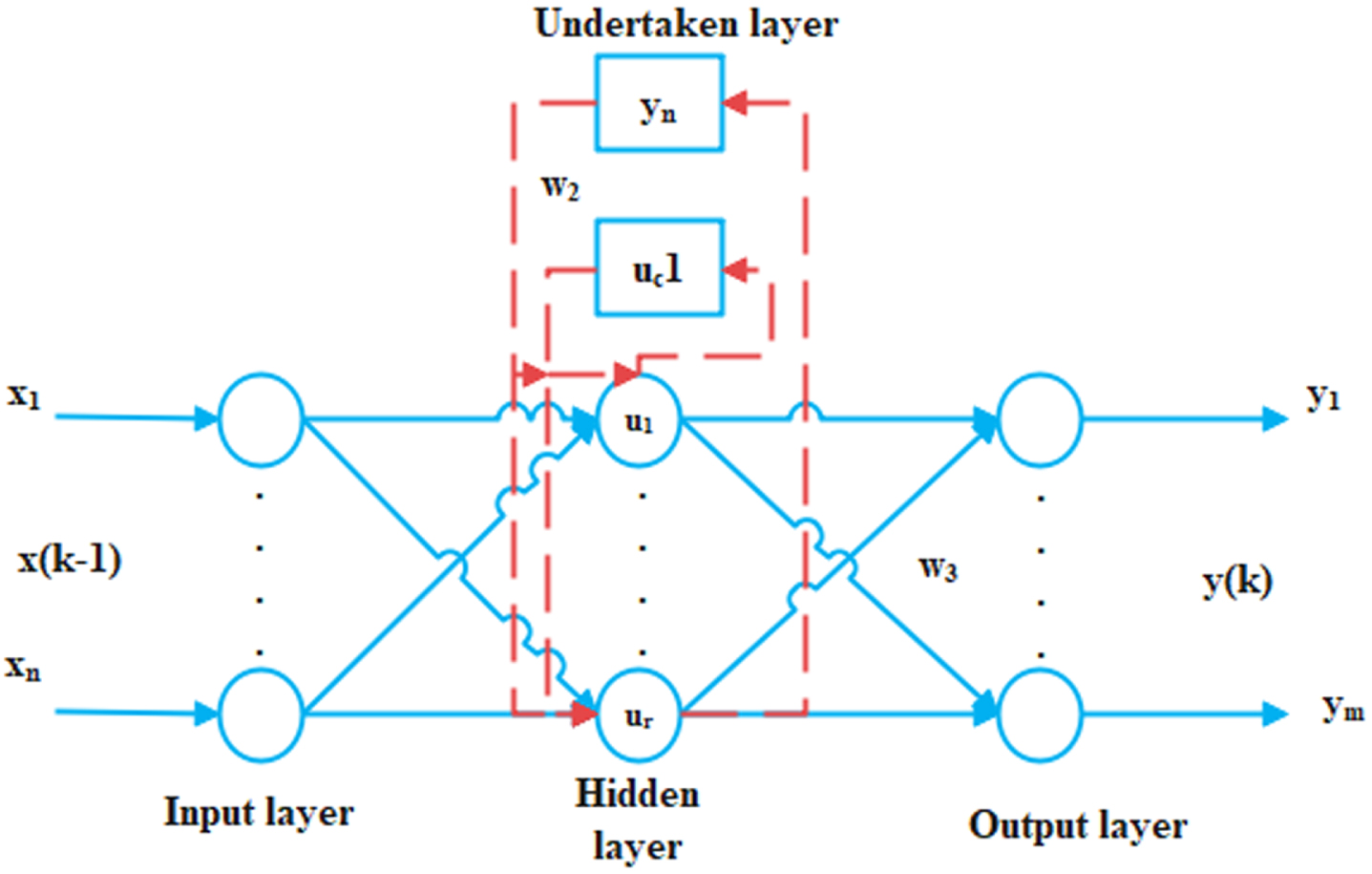
The output of the hidden components of its input by delaying and storing the company layer are based on the BP network. This joining is sensitive to past information and the network for interior input can increase the dynamic data management capacity. The internal state memorization allows for a dynamic planning method, which allows the system to adapt to temporal alterations across interval. [17].
The weight of the hidden layer input is w 1, the weight of the hidden layer in the layer is w2, the weight of the hidden layer to the output layer is w3; u (k - 1) is the input for the neural network; x (k) is the output for the hidden layer; y (k) is an output for a hidden layer, xc (k) is the output of the undertaking layer and y(k) is the output of that hidden layer. xc (k) is the output of the undertaking layer and
(4)
(5)
(6)
(7)
(8)
5.2Recurrent Neural Network (RNN)
Because of its extra feedback from the created layer output between input and output layers, RNN is an exclusive class of neural network.his layer is the context layer that retains data between observations [18]. In the present period, the results of the processing in the previous phase can be carried over and employed. Iparticular in real time applications, the fundamental characteristic of RNN offers an extremely large advantage. In adding to learning via all current inputs, RNN can have an unbounded memory level, and can thus learn connections over time [19]. The RNN is showed in Fig. 7.
Fig. 7
RNN Architecture.
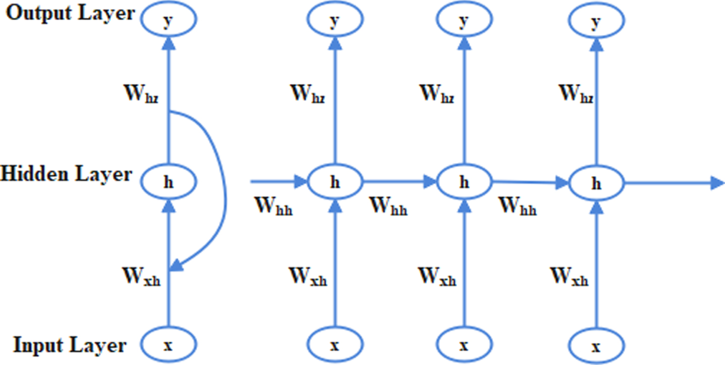
Hidden layer of Input is stated as in (9) as:
(9)
Here ht is represented as the hidden layer at the instance tth, Xt is represented as the input at instance tth, moreover, gn is represented as the function, and Wxh is represented as the input to hidden layer of weight matrix Equation (10) which characterizes the concealed to output layer is stated as:
(10)
3.5.3Cascade forward network
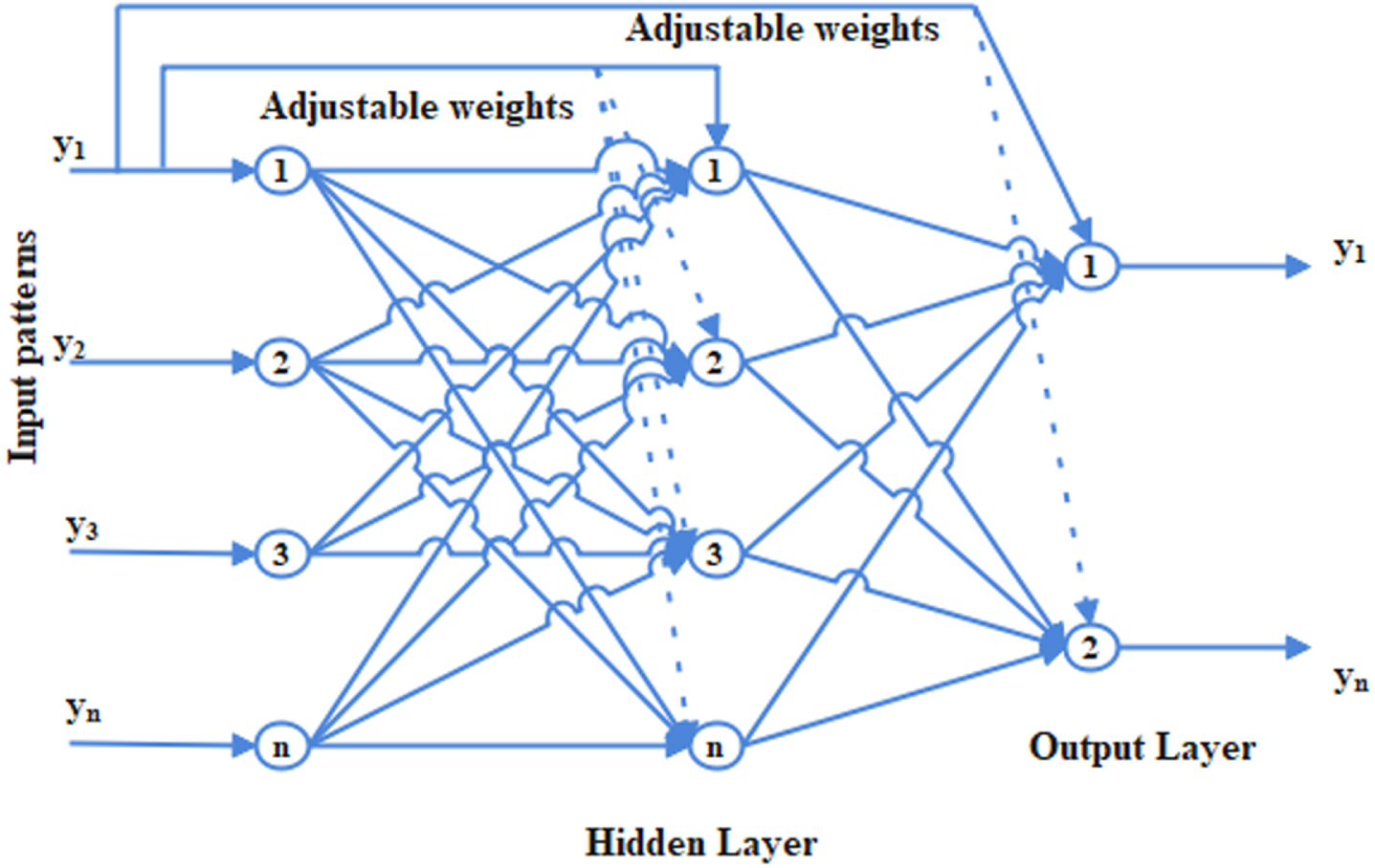
The Cascade Forward Network (CFN), which uses back propagation to update weights, has similarities with the FFNN. The primary dtinction ithat the connection between the individual level and the input at the next level is weighted [20]. In many circumstances, it has been thought that some cascade bpropagation can perform better than FFNN [21]. An important feature of this CFN is that each neuron layer is linked to the whole preceding neuron layer [22].The pictographic representation of CFN is in Fig. 8.
Fig. 8
Cascade FNN.
The CFN mathematical equation is specified as:
(11)
Input layer activation function is provided in the output layer as a fi, whereas input layer weight to output layer is
(12)
The next section will show the performance analysis of proposed model.
4Results and discussion
MLAB R2021a and Intel i5 processor, with 1Tera Byte hard disk and 8GB of RAM, is being explored with the projected system.
4.1Evaluation metrics
The challenge evaluation measurements are utilized tsurvey our method’s execution in division and classification. The assessment criteria for division incorporate sensitivity (SE), specificity (SP), accuracy (AC), and false measures. The presentation requirements are as follows:
(13)
(14)
(15)
(16)
(17)
(18)
(19)
Where tp, tn, fp and fn signify the true negative, false positive, number of a true positive TP, and false negative FN, N describes the total number of elements.
4.1Performance study of proposed FFNN model for 80% -20% of dataset
In this section, two different types of analysis are carried out by considereing with and without financial derivative features to validate the performance of proposed FFNN model with various neural networks. Initially, the available data is splits into 80% -20%, i.e. 80% of data is used for training procedure and remaining 20% of data is used for testing process. Table 3 provides the experimental value of different neural networks without financial derivative features for the analysis of 80% -20% in available dataset.
Table 3
Perfomance evaluation without financial derivative features
| Classification Technique | Sensitivity | Specificity | Precision | Recall | Gmean |
| ENN | 1.0000 | 0.8365 | 0.0582 | 1.0000 | 0.9146 |
| RNN | 1.0000 | 0.8160 | 0.0520 | 1.0000 | 0.9033 |
| CFNN | 1.0000 | 0.7988 | 0.0478 | 1.0000 | 0.8937 |
| FFNN | 1.0000 | 0.8572 | 0.0660 | 1.0000 | 0.9258 |
The above Table 3 validate the performance of projected model in terms of precision, specificity, recall, sensitivity and gmean. The sensitivity and recall are same for the all techniques, i.e. the ENN model achieved 1.000 of sensitivity and recall, where the proposed FFNN model achieved 1.000 of sensitivity and recall. In the specificity experiments, the ENN, RNN, CFNN and FFNN achieved 83%, 81%, 79% and 85%, which proves that the proposed FFNN achieved better performance than other neural networks. The ENN and RNN achieved nearly 91% of gmean, CFNN achieved 89% of gmean, but the proposed FFNN achieved 92% of gmean and high value of precision (i.e.0.0660). However, the existing neural network achieved only 0.0550 of precision value. From this study, the proposed FFNN model attained better presentation even without financial derivative features. Table 4 and Fig. 9 shows the performance of FFNN model in terms of accurateness and F-measure.
Table 4
Perfomance evaluation with financial derivative features
| Classification Technique | Sensitivity | Specificity | Precision | Recall | Gmean |
| ENN | 1.0000 | 0.8638 | 0.0690 | 1.0000 | 0.9294 |
| RNN | 1.0000 | 0.8864 | 0.0816 | 1.0000 | 0.9415 |
| CFNN | 1.0000 | 0.8586 | 0.0667 | 1.0000 | 0.9266 |
| FFNN | 1.0000 | 0.9085 | 0.0994 | 1.0000 | 0.9531 |
Fig. 9
Accuracy and F-measure Evaluation of FFNN Without Having Financial Derivative Features.
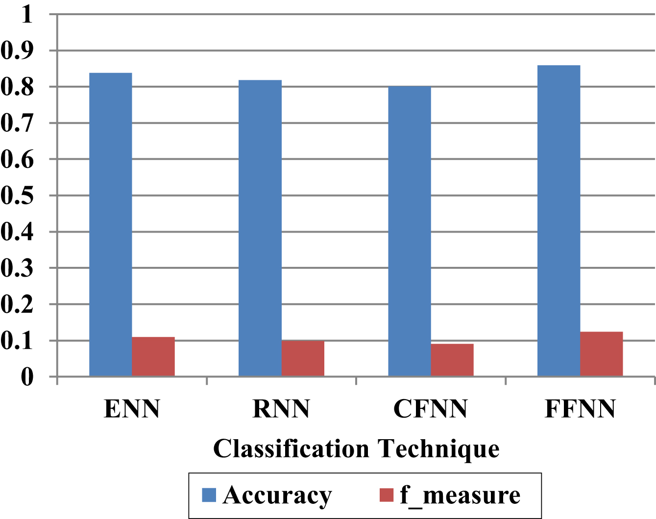
In the accuracy analysis of without having the financial derivative features, the ENN, RNN, CFNN and proposed FFNN achieved the 83%, 81%, 80% and 85%. As well as, these techniques achieved the f-measure of 0.11, 0.09, 0.09 and 0.12. From these analysis, it is clearly proved that without financial derivative features also, the proposed FFNN model achieved better performance for 80% -20% of available dataset. The next Table 5 shows the validation of proposed FFNN model with existing models by considering the financial derivative features for the 80% -20% of available dataset.
Table 5
Evaluation of FFNN model Without Having Financial Derivative Features
| Classification Models | Accuracy | F Measure |
| ENN | 0.8381 | 0.1100 |
| RNN | 0.8178 | 0.0989 |
| CFNN | 0.8008 | 0.0912 |
| FFNN | 0.8586 | 0.1239 |
In the specificity analysis, the ENN, RNN, CFNN and FFNN achieved 86%, 88%, 85% and 90%, where the sensitivity and recall of all techniques are 1.000, when implementing with financial derivative features. In the precision experiments, the FFNN achieved high performance (i.e. 0.0994), where the ENN and CFNN achieved nearly 0.0670. The ENN, RNN, CFNN and FFNN achieved gmeans of 92%, 94%, 92% and 95% that shows that the projected FFNN model achieved better presentation than other techniques. However, the FFNN achieved less performance, when it is not implemented with Financial Derivative features. This proves that these added features plays a major role for predicting the future IPEZ accurately. Table 6 and Fig. 10 shows the experimental investigation of proposed FFNN model in terms of accuracy and F-measure for the 80% -20% of available dataset.
Fig. 10
Performance Evaluation of Proposed FFNN With Financial Derivative Features for 80% -20% of available dataset.
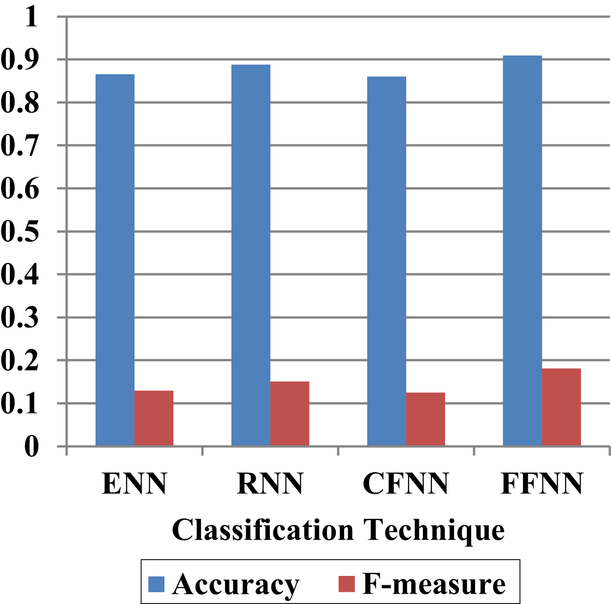
Table 6
Performance evaluation of proposed FFNN with financial derivative features
| Classification Models | Accuracy | F-measure |
| ENN | 0.8652 | 0.1292 |
| RNN | 0.8875 | 0.1509 |
| CFNN | 0.8600 | 0.1250 |
| FFNN | 0.9094 | 0.1808 |
In the accuracy analysis, the ENN and CFNN achieved low accuracy (i.e. nearly 86%), RNN achieved 88% and proposed FFNN achieved 90%. The ENN, RNN, CFNN and FFNN achieved the f-measure of 0.12, 0.15, 0.12 and 0.18 that proves FFNN achieved better performance than other neural techniques. Without financial derivative features, the proposed FFNN achieved less performance, which is proven in Tables 3 and 4. The next section will explain the experimental analysis for 60% -40% of existing dataset.
4.2Performance study of proposed FFNN model for 60% -40% of dataset
Here, the performance of projected FFNN technique is validated with the 60% of training data and 40% of testing statistics. Table 7 shows the analysis of FFNN in terms of several metrics without considering the financial derivative features.
Table 7
Perfomance evaluation of propsoed FFNN with financial derivative features
| Classification Models | Sensitivity | Specificity | Precision | Recall | Gmean |
| ENN | 1.0000 | 0.8027 | 0.0487 | 1.0000 | 0.8959 |
| RNN | 1.0000 | 0.8217 | 0.0536 | 1.0000 | 0.9065 |
| CFNN | 1.0000 | 0.7443 | 0.0380 | 1.0000 | 0.8627 |
| FFNN | 1.0000 | 0.8674 | 0.0708 | 1.0000 | 0.9314 |
The above table validate the performance of proposed model in terms of s ensitiveness, specificity, precision, recall and gmean. The sensitivity and recall are same for the all techniques, i.e. the RNN, CFNN model achieved 1.000 of sensitivity and recall, where the proposed FFNN model achieved 1.000 of sensitivity and recall. In the specificity experiments, the ENN, RNN, CFNN and FFNN achieved 80%, 82%, 74% and 86%, which proves that the proposed FFNN achieved better performance than other neural networks. The ENN and RNN achieved nearly 90% of gmean, CFNN achieved 86% of gmean, but the proposed FFNN achieved 93% of gmean and high value of precision (i.e.0.0708). However, the existing neural network achieved only 0.0450 of precision value. From this analysis, the proposed FFNN model achieved improved performance with financial derivative features. Table 8 and Fig. 11 shows the performance of FFNN model in terms of accurateness and F-measure with additional financial derivative features.
Table 8
Performance evaluation of proposed FFNN with financial derivative features
| Classification technique | Accuracy | F-measure |
| ENN | 0.8047 | 0.0929 |
| RNN | 0.8234 | 0.1017 |
| CFNN | 0.7469 | 0.0732 |
| FFNN | 0.8688 | 0.1322 |
Fig. 11
Evaluation of FFNN With Financial Derivative Features in terms of accurateness and F-measure.
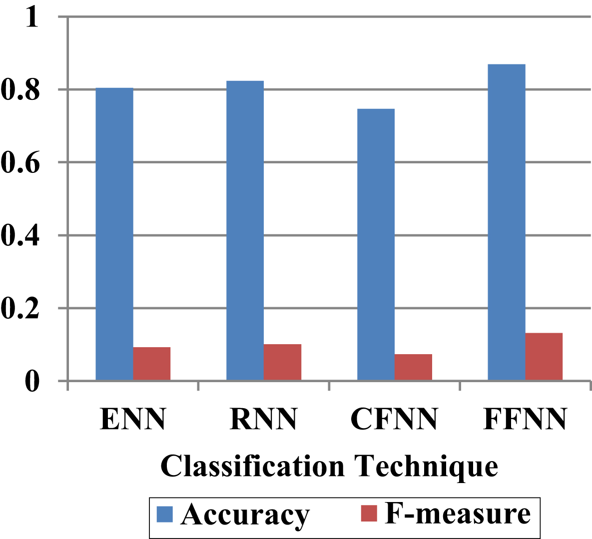
In the accurateness analysis of with the financial derivative features, the ENN, RNN, CFNN and proposed FFNN achieved the 80%, 82%, 74% and 86%. As well as, these techniques achieved the f-measure of 0.09, 0.10, 0.07 and 0.13. From these analysis, it is clearly proved that with financial derivative features also, the proposed FFNN model achieved higher performance for 60% -40% of available dataset. The next section will presents the analysis of future data prediction using proposed FFNN with other neural networks.
4.3Performance analysis of future data prediction
By using the available datasets, the proposed FFNN tries to predict the future IPFZ accurately in terms of exactness, recollection, sensitivity, specificity and gmean. This analysis is taken for 80% of training data and 20% of testing data and the experimental values are given in Table 9.
Table 9
Perfomance evaluation with financial derivative features
| Classification models | Sensitivity | Specificity | Precision | Recall | Gmean |
| ENN | 1.0000 | 0.5833 | 0.0237 | 1.0000 | 0.7638 |
| RNN | 1.0000 | 0.5423 | 0.0216 | 1.0000 | 0.7364 |
| CFNN | 1.0000 | 0.5013 | 0.0199 | 1.0000 | 0.7080 |
| FFNN | 1.0000 | 0.6449 | 0.0277 | 1.0000 | 0.8030 |
The sensitivity and recall are same for the all techniques, i.e. the ENN, RNN, CFNN model achieved 1.000 of sensitivity and recall, where the proposed FFNN model achieved 1.000 of sensitivity and recall. In the specificity experiments, the ENN, RNN, CFNN and FFNN achieved 58%, 54%, 50% and 64%, which proves that the proposed FFNN achieved better performance than other neural networks. The ENN, RNN and CFNN achieved nearly 75% of gmean, but the proposed FFNN achieved 80% of gmean and high value of precision (i.e.0.0277) than other neural networks (i.e.0.022 of precision). However, the CFNN achieved only 0.0199 of precision value. From this analysis, the projected FFNN model attained better performance with financial derivative features. Table 10 and Fig. 12 shows the performance of FFNN model in terms of accurateness and F-measure with additional financial derivative features.
Table 10
Evaluation of proposed FFNN with financial derivative features for future data
| Classification modules | Accuracy | F-measure |
| ENN | 0.5875 | 0.0462 |
| RNN | 0.5469 | 0.0423 |
| CFNN | 0.5062 | 0.0389 |
| FFNN | 0.6484 | 0.0538 |
Fig. 12
Evaluation of proposed FFNN With Financial Derivative Features for future data.
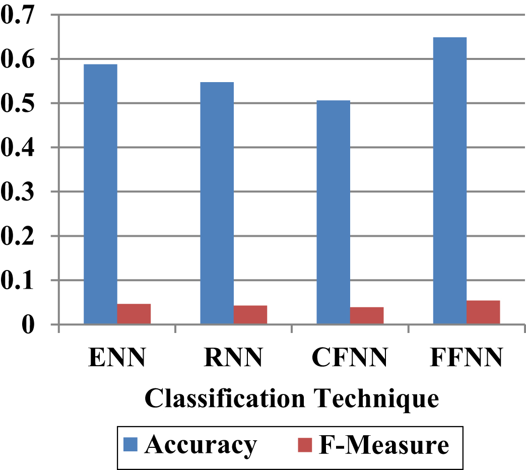
In the accuracy analysis of with the financial derivative features, the ENN, RNN, CFNN and proposed FFNN achieved the 58%, 54%, 50% and 64%. As well as, these techniques achieved the f-measure of 0.04, 0.04, 0.03 and 0.05. From this analysis, it is clearly proved that with financial derivative features also, the proposed FFNN model achieved higher performance for future data. However, the performance is less when compared with the analysis of 80% -20% and 60% -40% of data. The reason is that the layers of FFNN model is needs to improve for the prediction of future data.
4.4Comparative analysis of Proposed FFNN with various Existing approach
The above table clearly proves that the proposed FFNN model achieved better accuracy than various existing techniques. For example, the data mining approach [23] and HMM [24] achieved nearly 83% of accuracy, where SVM [25], RF [26] achieved nearly 79% of accuracy. But, the FFNN model achieved 90.94% of accuracy due to the usage of additional financial derivative features as input for predicting the future IPFZ accurately [27]. However, the performance needs improvement by modifying the layers of FFNN.
5Conclusion
Satellites assist detect environmental elements that affect fish habitat. Satellite observations Surface temperature, water colour, wind and current data comprise environmental characteristics that are well measured using satellite sensor data. Fern sensing data are used to obtain information on chlorophyl content, primary productivity, coastal and estuarine bio optical qualities and ocean traffic characteristics. In this research study, OST dataset is used for future prediction. Initially, 13 features are used as input and after that financial derivative features are added with those 13 features for accurate future prediction of IPFZ. These more number of features are given as input to FFNN and compared with ELN, RNN and CFNN. The validation results proves that the FFNN achieved better performance than other neural network techniques and less performance for future data analysis. From this analysis, it is proved that more of the research articles are not supporting for this PFZs future forecast (Table 11). In this work we are major concentrated on the PFZs future forecast, which leads the average accuracy of FFNN model. In future, the performance can be improved by implementing the ensemble classifiers with financial derivative features.
Table 11
Comparative analysis of with various existing approach
| Author Year | Approach | Data used | Accuracy averaged |
| Natteshan et al [22] 20161 | Data mining approach | Fishery, SSC, OST data from 2000-2004 | 87.11 |
| Natteshan et al [22] 20162 | Heuristic Rule approach | SSC, OST and turbidity | 84.71 |
| de Souza et al 2016 [23] | A Hidden Markov Model (HMM) | S-AIS | 83 |
| da Silveira et al 2021 [24] | SVM | – | 79 |
| Naghibi et al. 2016 [25] | Regression tree, and random forest machine learning models | — | 78.03 |
| Proposed 2021 | FFNN with Financial Derivative Features | OST | 90.94 |
Note
Funding sources
Not available for this Research Article.
References
[1] | Shailesh Nayak , Solanki H.U. and Dwivedi R.M. , Utilization of IRS P4 ocean colour data for potential fishing zone— a cost benefit analysis, ((2003) ). |
[2] | Wagiyo K. , Pane A.R.P. and Chodrijah U. , Parameter populasi, aspek biologi dan penangkapan tongkol komo (Euthynnus affinis Cantor, di Selat Malaka [Population parameters, biological aspects and catching mackerel tuna (Euthynnus affinis) in Malacca Strait], IFRJ 23: (4) ((2017) ), 287–297. |
[3] | Raja R. Kumar Vinston , Krishnan K. Ashok , and Gokula V. , Condition based Ensemble Deep Learning and Machine Learning Classification Technique for Integrated Potential Fishing Zone Future Forecasting, International Journal on Recent and Innovation Trends in Computing and Communication 11: (2), ((2023) ) 75–85, ISSN 23218169, 10.17762/ijritcc.v11i2.6131. |
[4] | Solanki H.U. , Raman M. , Kumari B. , Dwivedi R.M. and Narain A. , Seasonal trends in the fishery resources off Gujarat: Salient observation using NOAA AVHRR, 2016. |
[5] | Tummala S.K. , Masuluri N.K. , Nayak S. and Benefits December. , derived by the fisherman using Potential Fishing Zone (PFZ) advisories. In Remote Sensing of Inland, Coastal, and Oceanic Waters (Vol. 7150: p. 71500N). International Society for Optics and Photonics (2008) . |
[6] | Rahul P.R.C. , Sahu S.K. and Salvekar P.S. , Interlacing ocean model simulations and remotely sensed biophysical parameters to identify integrated potential fishing zones, IEEE Geoscience and Remote Sensing Letters 8: (4) ((2011) ), 789–793. |
[7] | Solanki H.U. , Dwivedi R.M. , Nayak S.R. , Gulati D.K. , John M.E. and Somvanshi V.S. , Potential fishing zones (PFZ) forecast using satellite data derived biological and physical processes, Journal of the Indian Society of Remote Sensing 31: (2) ((2003) ), 67–69. |
[8] | Abiodun O.I. , Jantan A. , Omolara A.E. , Dada K.V. , Mohamed N.A. and Arshad H. , State-of-the-art in artificial neural network applications: A survey, Heliyon 4: (11) ((2018) ), p. e00938. |
[9] | Mustapha A.M. , Chan Y.L. and Lihan T. , Mapping of Potential Fishing Grounds of Rastrelliger Kanagurta (Cuvier, using Satellite Images, Map Asia2010& ISG 2010 Symposium, pp. 26–28 (2010) . |
[10] | Chang Y. Sun Chi-Lu , Chen Yong , Yeh Su-Zan and Dinardo Gerard , Habitat suitability analysis and identification of potential fishing grounds for swordfish, Xiphias gladius, in the South Atlantic Ocean, International Journal of Remote Sensing 33: (23) ((2012) ), 7523–7541. |
[11] | Zainuddin M. , Katsuya Saitoh and Sei-Ichi Saitoh, Albacore (Thunnus alalunga) fishing ground in relation to oceanographic conditions in the western North Pacific Ocean using remotely sensed satellite data, Fish. Oceanogr. 17: (2) ((2008) ), 61–73. |
[12] | Daqamseh Salleh T , Mansor Shattri , Pradhan Biswajeet , Billa Lawal and Mahmud Ahmad Rodzi , Potential fish habitat mapping using MODIS-derived sea surface salinity, temperature and chlorophyll-a data: South China Sea Coastal areas, Malaysia, Geocarto International, Vol. First article, pp. 1–15, (2012) . |
[13] | Semedi B. and Dimyati R.D. , Study on Mackerel catch, Sea Surface Temperature and Chlorophyll – a in the Makassar strait, International Journal of Remote Sensing and Earth Sciences 6: ((2009) ), 77–84. |
[14] | Sam Cramer and Michael Kampouridis and Alex A. Freitas , Feature Engineering for Improving Financial Derivatives-based Rainfall Prediction, In: IEEE World Congress on Evolutionary Comutation, 24-29 Jul 2016 Vancouver, Canada ((2016) ). |
[15] | Raja R. Vinston and Kumar K. Ashok , Fisher Scoring with Condition-based Ensemble Supervised Learning Classification Technique for Prediction in PFZ Journal of Uncertain Systems VOL. 0, NO. ja https://doi.org/10.1142/S1752890922410094 |
[16] | Elman J.L. , Finding structure in time, Cognitive Science 14: (2) ((1990) ), 179–211. |
[17] | Jia W. , Zhao D. , Shen T. , Tang Y. and Zhao Y. , Study on optimized Elman neural network classification algorithm based on PLS and CA,, Computational Intelligence and Neuroscience ((2014) ). |
[18] | Lashkarbolooki M. , Shafipour Z.S. and Hezave A.Z. , Trainable cascade-forward back-propagation network modeling of spearmint oil extraction in a packed bed using SC-CO2, The Journal of Supercritical Fluids 73: ((2013) ), 108–115. |
[19] | Chauhan B.K. , Sharma A. and Hanmandlu M. , Neuro-Fuzzy Approach Based Short Term Electric Load Forecasting, In 2005 IEEE/PES Transmission & Distribution Conference & Exposition: Asia and Pacific (pp. 1–5), ((2005) , August). |
[20] | Lashkarbolooki M. , Vaferi B. , Shariati A. and Hezave A.Z. , Investigating vapor– liquid equilibria of binary mixtures containing supercritical or near-critical carbon dioxide and a cyclic compound using cascade neural network, Fluid Phase Equilibria 343: ((2013) ), 24–29. |
[21] | Filik U.B. and Kurban M. , A new approach for the short-term load forecasting with autoregressive and artificial neural network models, International Journal of Computational Intelligence Research 3: (1) ((2007) ), 66–71. |
[22] | Beale M.H. , Hagan M.T. and Demuth H.B. , Neural network toolbox user’s guide, The Math Works Inc 103: ((1992) ). |
[23] | Natteshan N.V.S. and Suresh N.K. , A survey of various methods of potential fishing zone identification, International Journal of Control Theory and Applications 9: (40) ((2016) ), 697–703. |
[24] | de Souza E.N. , Boerder K. , Matwin S. and Worm B. , Improving fishing pattern detection from satellite AIS using data mining and machine learning, PloS One 11: (7) ((2016) ), p.e0158248. |
[25] | da Silveira C.B.L. , Strenzel G.M.R. , Maida M. , Gaspar A.L.B. and Ferreira B.P. , Coral Reef Mapping with Remote Sensing and Machine Learning: A Nurture and Nature Analysis in Marine Protected Areas, Remote Sensing 13: (15) ((2021) ), 2907. |
[26] | Raja, R. Vinston and Kumar, K. Ashok , Collision Averting Approach in Deep Maritime Boats using Prophecy of Impact Direction, 5th International Conference on Trends in Electronics and Informatics, ICOEI 2021 Pages 1066–10713 June 2021 Article number 9453084, ICOEI 2021. Tirunelveli, Tamilnadu, ISBN: 978-166541571-2, DOI: 10.1109/ICOEI51242.2021.9453084. |
[27] | Naghibi S.A. , Pourghasemi H.R. and Dixon B. , GIS-based groundwater potential mapping using boosted regression tree, classification and regression tree, and random forest machine learning models in Iran, Environmental Monitoring and Assessment 188: (11) ((2016) ), 1–27. |


