
An integrated decision-making methodology for green supplier selection based on the improved IVIF-CPT-MABAC method
Abstract
Green supply chain management attaches great importance to the coordinated development of social economy and ecological environment, and requires enterprises to consider environmental protection factors in product design, packaging, procurement, production, sales, logistics, waste and recycling. Suppliers are the “source” of the entire supply chain, and the choice of green suppliers is the basis of green supply chain management, and their quality will directly affect the environmental performance of enterprises. The green supplier selection is a classical multiple attribute group decision making (MAGDM) problems. Interval-valued intuitionistic fuzzy sets (IVIFSs) are the extension of intuitionistic fuzzy sets (IFSs), and are utilized to depict the complex and changeable circumstance. To better adapt to complex environment, the purpose of this paper is to construct a new method to solve the MAGDM problems for green supplier selection. Taking the fuzzy and uncertain character of the IVIFSs and the psychological preference into consideration, the original MABAC method based on the cumulative prospect theory (CPT) is extended into IVIFSs (IVIF-CPT-MABAC) method for MAGDM issues. Meanwhile, the method to evaluate the attribute weighting vector is calculated by CRITIC method. Finally, a numerical example for green supplier selection has been given and some comparisons is used to illustrate advantages of IVIF-CPT-MABAC method and some comparison analysis and sensitivity analysis are applied to prove this new method’s effectiveness and stability.
1Introduction
The concept of fuzzy sets (FSs) proposed by Zadeh [1] descripts the complex decision-making environment, and it has been extended into more complicated fuzzy sets such as IFSs [2, 3] and the hesitant fuzzy set (HFS) [4] which are the two main branches of FSs. The IFSs is the classical fuzzy set and it has been applied to many fields, such as business management, decision -making and so on [5–7]. Constrained by the fact that the IFSs is in the range of real number, the IVIFSs is the extension of IFSs with the interval numbers to express the membership and non-membership degree which could satisfy the increasingly complex decision environments. Thus, Atanassov [8] proposed the conception of IVIFSs, and the corresponding operators of IVIFSs are the introduced [9]. With the basic research set up, the corresponding innovation of IVIFSs has been proposed [10–14]. Mondal and Samanta [15] defined the topology and studied the characteristic of IVIFSs which could prove the IVIFSs could construct the topological category. Grzegorzewski [16] defined new distance method based on Hausdorff metric which is the well-known Hamming distance. Xu [17] based on some operational laws of IVIFSs, such as the score function and accuracy, gave the introduction of geometric aggregation operator. Zhang, Dong, Zhang and Song [18] introduced the inclusion and similarity measure in IVIFSs. Senapati, Chen, Mesiar and Yager [19] proposed novel Aczel-Alsina operations and applied it in the MADM process. Besides, the latest research on IFSs and IVIFSs in MADM is enough to attract everyone’s attention. For instance, Hayat et al. proposed the new aggregation operators on group-based generalized intuitionistic fuzzy soft sets [20]; Karaaslan explored new aggregation operators on group-based generalized intuitionistic fuzzy soft sets from a new perspective [21]; Hayat et al. applied the new group-based generalized interval-valued q-rung orthopair fuzzy soft aggregation operator to sports decision-making problems, and extended the generalized intuitionistic fuzzy soft set [22–24]; Yang et al. explored the application of aggregation and interactive aggregation soft operators under the interval-valued q-order orthomorphic fuzzy soft environment in the evaluation of automation companies [25] and so on. Meanwhile, many MADM methods have been developed into IVIFSs to solve the practical MADM problems. TOPSIS method [26], grey relational analysis (GRA) method [27, 28], maximizing deviation method [29], VIKOR method [30, 31], MABAC method [13, 32], and so on.
MADM contains multiple criteria, conflict among criteria, incommensurable units, alternatives and preference decision [33, 34]. Group decision making (GDM) means one more decision-makers (DMs) to take part in the decision-making progress [35], and means the results do not determined by one DM. The MAGDM is the integration of MADM and GDM which means the multi-attribute decision making is made by one more DM. Thus, MAGDM problems are too scientific and complex to evaluate by simple real number and operation. The FSs and its extension provide to contain more information [36–39] and MADM methods provide different theories to evaluate the attribute weight and the alternatives [40–43]. Different from other methods, MABAC [44] evaluates the alternative by defining the distance between possible solution and border approximation area, and is a classical method utilized in different fuzzy sets which include Pythagorean Fuzzy sets (PFSs) Peng and Yang [45], interval neutrosophic sets (INSs) [46], interval type-2 fuzzy [47]. The above studies all consider the assumption that DMs are all rational. However, in the practical situation, the psychological preference should be fully considered for the influence on decision outcomes. According to the related theory, such as CPT [48], DMs are always risk-averse.
Selecting long-term stable suppliers is the most important problem in building a green supply chain under the green supply chain management mode, which directly affects the competitiveness of enterprises in the market [49–51]. How to grasp the changing internal and external environment, determine reasonable evaluation indicators according to their own needs, and choose green suppliers that suit them has become an urgent problem to be solved [52–54]. The selection of green suppliers is a process of coordinating with the economic benefit objective on the basis of considering environmental factors and giving them certain weights. The selection process of green suppliers can neither overemphasize environmental protection factors, nor overemphasize economic interests. Only by coordinating the development of the two, can the long-term cooperation between enterprises and suppliers be promoted. Green supplier selection is a very complex decision-making problem [55–58]. Due to the complexity of the green supply chain system and the uncertainty, ambiguity and hesitation of human thinking, the evaluation of green suppliers will be affected by many uncertain factors, which makes it difficult to describe the evaluation indicators with exact values [59–62]. In order to be more in line with the thinking and cognitive mode of decision makers, this paper uses IVIFSs to describe attribute values. With the rapid development of science and technology, many decision-making problems in life have become more and more complex, and it is difficult to better solve these problems by relying solely on a certain decision-maker. The MAGDM together not only to reduce mistakes, but also to improve the accuracy of decision-making. It can be seen that it is of great significance to apply the MAGDM method under IVIFS to the selection of green suppliers. Therefore, it is necessary to integrate the CPT which takes the DMs’ risk preference into consideration and classical MAGDM methods. In this study, the concepts of IVIFS, MABAC and some distance in interval-value intuitionistic fuzzy environment are reviewed, however, some problems are also found in the review process. The motivations of this study are put forward as follows: (1) In the face of increasingly complex decision-making environment and complicated reality, it is particularly important to obtain evaluation information efficiently. IVIFS can more flexibly and completely express the preference evaluation information of DMs. (2) Since the existing CRITIC method is only applicable to real numbers, this paper uses precise functions to extend CRITIC algorithm to IVIFS environment to improve the rationality of attribute weight information. (3) Selecting good green suppliers has a far-reaching positive impact on promoting the improvement of green supply chain management and the development of green economy. (4) The method proposed in this paper can effectively solve the MAGDM problems which the decision-making information is expressed by IVIFSs and the attributes have local advantages.
The aim of this paper is to extend MABAC method based on CPT for MAGDM under IVIFSs and apply it into green supplier selection. The contributions of this paper are shown as follows: (1) The integration of CPT and MABAC method in IVIFSs which not only considers relatively simple and reasonable classical method, but also considers the psychological state of DMs which is more realistic has been constructed. This new method has clear decision-making logic and stable results, which makes the new theory more practical. (2) The CRITIC method is extended into IVIFSs to calculate the weighting vector of attributes, making the method proposed in this paper more practical. (3) the IVIF-CPT-MABAC method is not only proposed for MAGDM issues, but also broadens the practical application range of IVIF theory. (4) Finally, a numerical example of green supplier selection is built to illustrate the practicality of the proposed and some comparisons is used to illustrate advantages of IVIF-CPT-MABAC method and some comparison analysis and sensitivity analysis are applied to prove this new method’s effectiveness and stability.
The following is the structure of the article. Section 2 gave the basic introduction and calculation operators of IVIFSs and the classical CPT. In section 3, the IVIF-CPT-MABAC method is constructed for MAGDM and is applied into green supplier selection in Section 4. Meanwhile, Section 4 gave a numerical example for green supplier selection and gave the sensitivity and comparison analysis to prove this method’s stability and effectiveness. In the conclusion, we prospect the application of this new method.
2Preliminary knowledge
In this section, the basic elements related to decision-making such as IVIFS and CPT are described below.
2.1IVIFSs
IVIFS, as an extension of the IFS, breaks the limitation of IFS on the representation of real numbers and makes information description more accurate and scientific. In IVIFS, the membership, non-membership and hesitancy degree are depicted with interval value for the complexity and uncertainty of objective things. The specific definition is depicted as follows.
Definition 1. [63]. Let Y be a finitely nonempty set, and the IFS is described as Equation (2.1):
(2.1)
(2.2)
(2.3)
(2.4)
(2.5)
Definition 2 [8]. Let Y be a finitely nonempty set, then the IVIFS is described as follows:
(2.6)
(2.7)
(2.8)
(2.9)
Similarity, the hesitancy degree of IVIFS is shown as follows:
(2.10)
The interval-valued intuitionistic fuzzy numbers (IVIFN) in Equation (2.6) are shown as follows:
(2.11)
Which could be abbreviated to the form in Equation (2.12)
(2.12)
Specially, when LM = RM, LN = RN, IVIFS degenerate into IFS. The maximum IVIFN is
Definition 3 [17]. Suppose any three IVIFNs,
(1)
(2)
(3)
(4)
(5)
(i) Commutative law
a)
b)
(ii) Associative law
a)
b)
(iii) Distributive law
a)
b)
(iv) Exponential operation law
a)
b)
where λ, λ1, λ2, ⩾ 0.
Definition 4 [64]. Let
(2.13)
where
(2.14)
where
Definition 5 [64]. According to Definition 4, suppose any two IVIFNs,
If
If
If
a) If
b) If
c) If
Definition 6 [17]. Let a set of m-dimensional fuzzy numbers be set
(2.15)
where ω = (ω1, ω2, …, ωm) T is the weighting vector of
Specially, if
Definition 7 [17]. Set
(2.16)
Specially, if
Definition 8 [16, 65]. Set two IVIFNs
(2.17)
(2.18)
(2.19)
2.2Cumulative prospect theory
There are mainly two kinds of risk decision-making theories in uncertain environment. One is expected utility theory, which assumes that people are in a completely rational state when making risk decisions, and this is also the common cognition of many scholars before the prospect theory is put forward. The other is prospect theory (PT) developed by Tversky and Kahneman [66] on the basis of bounded rationality theory in 1979. It realizes the influence of DMs’ risk preference on decision-making by comparing reference points, that is, when decision makers face risks, The sensitivity to loss is greater than the sensitivity to gain There are mainly two kinds of risk decision making theories in uncertain environment. One is expected utility theory, which assumes that people are in a completely rational state when making risk decisions, and this is also the common cognition of many scholars before the prospect theory is put forward. The other is PT on the basis of bounded rationality theory in 1979 [66]. It realizes the influence of decision maker’s risk preference on decision making by comparing reference points, that is, when decision makers face risks. The sensitivity to “loss” is greater than the sensitivity to “gain”. Such measures, which add to the psychology of policymakers, are more realistic. In 1992, Tversky and Kahneman [48] proposed the cumulative prospect theory (CPT) on the basis of prospect theory through a large number of experiments, which mainly improved and extended the scope of application to decision-making situations with arbitrary number of results and random dominance problems. Such measures, which add to the psychology of policymakers, are more realistic.
The prospect function P (z) combined with value function V (z ɛ) and weighting function I (r ɛ), and its expression formula is as Equation (2.20) [66].
(2.20)
A value function described by a piecewise function can be presented as Equation (2.21) [66].
(2.21)
When facing with gains and losses, the weighting function are shown as follows [66]:
(2.22)
3Extended MABAC method for MAGDM based on CPT under IVIFSs
In 2015, Pamučar and Ćirović [67] firstly proposed multi-attributive border approximation area comparison (MABAC). MABAC method defines the distance between alternative and the border approximation are (BAA), and divides the BAA into positive and negative BAA according to the value of distance. In the end, the final ranking results are determined by the equations. MABAC method has the character of simple, logic and feasible.
3.1Classical MABAC method
Suppose that in some multi-attribute decision-making problem, there are the set of alternatives ML = {ML1, ML2, ⋯ , MLn}, the set of attributes MT = {MT1, MT2, ⋯ , MTs} and the weighting vector of attributes ω = (ω1, ω2, ⋯ , ωs) T, and ∀ωj ∈ [0, 1],
(3.1)
The specific steps of classical MABAC method are as follows:
Step 1. Normalized decision.
Normalize the decision matrix X = [xij] n×s using Equation (3.2) and get normalized decision matrix
(3.2)
Step 2. Weighted normalized decision matrix.
The normalized decision matrix is determined by step 1, and with the weighting vector ω = (ω1, ω2, ⋯ , ωs) T, and the weighted normalized decision matrix
Step 3. The boundary approximates area value matrix.
The 1 × s boundary approximates area value matrix BAA = [gj] 1×s is obtained using Equation (3.3)
(3.3)
Step 4. Calculate the distance between BAA.
The distance Dqij between alternative MLi under each attribute and BAA are calculated as follows:
(3.4)
Step 5. Obtain the overall distance between alternative MLi and BAA.
(3.5)
Step 6. Rank the alternatives.
Rank all the alternatives MLi (i = 1, 2, ⋯ , n) according to the overall distance Si (i = 1, 2, ⋯ , n). If the value of overall distance Si is larger, the corresponding alternative is better. Otherwise, it indicates that the corresponding alternative is far from the standard and should be abandoned.
3.2The extended MABAC method for MAGDM based on CPT under IVIFSs
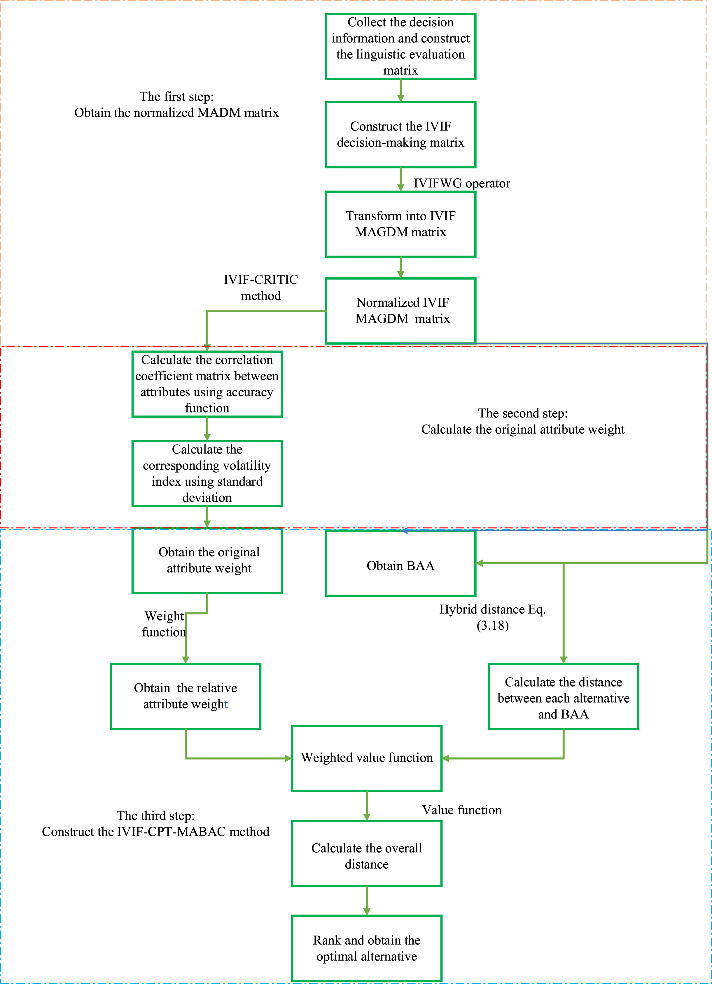
The integration of CPT and MABAC method takes the DMs’ psychological factor into consideration. The weighting vector is calculated by CRITIC method [68] calculates and the CPT-MABAC method is then extended in the IVIFSs. Thus, the extended CPT-MABAC applies IVIFNs to express information and extends the application range of MABAC method which is more in line with the uncertainty of the real environment. By the previously mentioned, the specific steps of IVIF-CPT-MABAC model for MAGDM are shown in Fig. 3.1.
Fig. 3.1
The framework of IVIF-CPT-MABAC method.
According to the IVIF correlation theory, the decision matrix is reconstructed based on PT. Suppose that there are a set of experts MD = {MD1, MD2, ⋯ , MDe}, a set of alternatives ML = {ML1, ML2, ⋯ , MLn}, and a set of attributes MT = {MT1, MT2, ⋯ , MTs}. The weighting vector of attributes ω = (ω1, ω2, ⋯ , ωs) T, and ∀ωj ∈ [0, 1],
(3.6)
Step 1. IVIF MAGDM matrices Q.
Equation (3.7) is determined by the IVIFWA operators to aggerate the IVIF MADM matrices
(3.7)
Step 2. Obtain the normalized IVIF MADM decision matrix Q′.
The normalized IVIF decision matrix
(3.8)
Step 3. Use the extended CRITIC method to get the original attribute weight.
The IVIF-CRITIC method is mainly divided into the following steps:
(i) Determine the correlation coefficient matrix R = [RCjp] s×s of attribute MTj and MTp using Equation (3.9)
(3.9)
(3.10)
(3.11)
(ii) Determine volatility index DXj.
a. Calculate the standard deviation σj of each attribute MTj.
(3.12)
b. Calculate the volatility index DXj of each attribute.
(3.13)
c. Determine the initial attributes weight ωj.
(3.14)
Step 4. Determine BAA.
According to the information in normalized IVIF decision matrix Q′, the
(3.15)
Step 5. Calculate the relative attribute weight matrix
Compare the magnitude of IVIFNs
(3.16)
Step 6. Obtain the weighted value function
(3.17)
(3.18)
Step 7. Obtain the overall distance
(3.19)
Step 8. Rank all the alternatives according to the overall distance
4Application of IVIF-CPT-MABAC method in GSS
4.1Background description
The concept of green supply chain was first proposed by the Manufacturing Research Association (MRC) of Michigan State University in 1996. It is a modern management mode that has the least negative impact on the environment and the most efficient use of resources [69–71]. In recent years, with the continuous occurrence of extreme weather, development and environmental protection should always keep pace, especially Chinese government has put forward the strategic requirement of sustainable development. Therefore, implementing green supply chain management is a sustainable development approach combining green consciousness and economic development [72, 73]. Again because of the green supplier located in the upstream of the supply chain, for the green supply chain had a significant influence on environmental protection and resource conservation, is an important part of the green supply chain management, so in this section, we based on IVIFSs environment, constructs to the third quarter of the model is applied to green supplier selection. As we all know, the GSS is a classical MAGDM issue [74–77]. To select the most appropriate green supplier, we invite five experts MDc (c = 1, 2, ⋯ , 5) to evaluate alternatives MLi (i = 1, 2, ⋯ , 5) under six attributes MTj (j = 1, 2, ⋯ , 6). By summarizing the relevant literature, the main six attributes are shown as follows: MT1: green manufacturing process; MT2: waste management; MT3: green Product design; MT4: green image; MT5: resource consumption; MT6: green environmental management system. MT2 and MT5 are negative attribute, and the weighting vector of experts is ϑ = (ϑ1, ϑ2, ⋯ , ϑ5) = (0.27, 0.16, 0.23, 0.16, 0.18). In order to be more in line with the realistic evaluation environment, we ask the experts to express their evaluation views clearly in language, and collect the evaluation of the experts to form the initial language evaluation matrix in Tables 4.2–4.6. Then according to the IVIF linguistic evaluation scale in Table 4.1, the expert’s literal language is transformed into an IVIFN adapted to our model, and the results are shown in Tables 4.7–4.11.
Table 4.2
The linguistic evaluation matrix given by the first expert
| MT1 | MT2 | MT3 | MT4 | MT5 | MT6 | |
| ML1 | G | VG | M | MG | MT | MG |
| ML2 | G | M | G | M | M | G |
| ML3 | EG | MG | PG | VG | M | VG |
| ML4 | MG | G | VG | B | G | VB |
| ML5 | VG | B | EG | PB | MG | VB |
Table 4.3
The linguistic evaluation matrix given by the second expert
| MT1 | MT2 | MT3 | MT4 | MT5 | MT6 | |
| ML1 | MG | VG | M | G | M | G |
| ML2 | G | M | G | MG | M | G |
| ML3 | PG | G | EG | EG | M | VG |
| ML4 | MG | G | VG | MB | MG | VB |
| ML5 | G | B | VG | B | MG | B |
Table 4.4
Linguistic evaluation matrix given by the third expert
| MT1 | MT2 | MT3 | MT4 | MT5 | MT6 | |
| ML1 | G | G | M | G | M | MG |
| ML2 | MG | M | G | M | B | MG |
| ML3 | EG | G | VG | VG | MG | PG |
| ML4 | MG | MG | G | M | G | B |
| ML5 | MG | MB | VG | MB | M | MB |
Table 4.5
Linguistic evaluation matrix given by the fourth expert
| MT1 | MT2 | MT3 | MT4 | MT5 | MT6 | |
| ML1 | MG | G | M | MG | MB | MG |
| ML2 | MG | M | MG | G | M | G |
| ML3 | EG | G | PG | VG | MG | EG |
| ML4 | G | G | G | M | G | B |
| ML5 | G | M | G | M | G | B |
Table 4.6
Linguistic evaluation matrix given by the fifth expert
| MT1 | MT2 | MT3 | MT4 | MT5 | MT6 | |
| ML1 | G | VG | M | MG | MB | MG |
| ML2 | VG | M | G | M | MG | G |
| ML3 | EG | M | PG | VG | M | VG |
| ML4 | G | G | VG | M | G | VB |
| ML5 | VG | B | EG | B | MG | VB |
Table 4.1
4.1 IVIF linguistic evaluation scale
| Linguistic scale | IVIFN |
| Perfectly bad (PB) | 〈 [0.00, 0.10] , [0.85, 0.90]〉 |
| Very bad (VB) | 〈 [0.00, 0.10] , [0.70, 0.75]〉 |
| Bad (B) | 〈 [0.15, 0.25] , [0.55, 0.60]〉 |
| Middle bad (MB) | 〈 [0.30, 0.40] , [0.45, 0.50]〉 |
| Middle (M) | 〈 [0.40, 0.50] , [0.35, 0.40]〉 |
| Middle good (MG) | 〈 [0.50, 0.60] , [0.25, 0.30]〉 |
| Good (G) | 〈 [0.60, 0.70] , [0.15, 0.20]〉 |
| Very good (VG) | 〈 [0.70, 0.80] , [0.05, 0.10]〉 |
| Extremely good (EG) | 〈 [0.80, 0.90] , [0.05, 0.10]〉 |
| Perfectly good (PG) | 〈 [1.00, 1.00] , [0.00, 0.00]〉 |
Table 4.7
The IVIF evaluation matrix Q(1) given by the first expert
| MT1 | MT2 | MT3 | |
| ML1 | 〈 [0.60, 0.70] , [0.15, 0.20]〉 | 〈 [0.70, 0.80] , [0.05, 0.10]〉 | 〈 [0.40, 0.50] , [0.35, 0.40]〉 |
| ML2 | 〈 [0.60, 0.70] , [0.15, 0.20]〉 | 〈 [0.40, 0.50] , [0.35, 0.40]〉 | 〈 [0.60, 0.70] , [0.15, 0.20]〉 |
| ML3 | 〈 [0.80, 0.90] , [0.05, 0.10]〉 | 〈 [0.40, 0.50] , [0.35, 0.40]〉 | 〈 [1.00, 1.00] , [0.00, 0.00]〉 |
| ML4 | 〈 [0.50, 0.60] , [0.25, 0.30]〉 | 〈 [0.60, 0.70] , [0.15, 0.20]〉 | 〈 [0.70, 0.80] , [0.05, 0.10]〉 |
| ML5 | 〈 [0.70, 0.80] , [0.05, 0.10]〉 | 〈 [0.15, 0.25] , [0.55, 0.60]〉 | 〈 [0.80, 0.90] , [0.05, 0.10]〉 |
| MT4 | MT5 | MT6 | |
| ML1 | 〈 [0.50, 0.60] , [0.25, 0.30]〉 | 〈 [0.30, 0.40] , [0.45, 0.50]〉 | 〈 [0.50, 0.60] , [0.25, 0.30]〉 |
| ML2 | 〈 [0.40, 0.50] , [0.35, 0.40]〉 | 〈 [0.40, 0.50] , [0.35, 0.40]〉 | 〈 [0.60, 0.70] , [0.15, 0.20]〉 |
| ML3 | 〈 [0.70, 0.80] , [0.05, 0.10]〉 | 〈 [0.40, 0.50] , [0.35, 0.40]〉 | 〈 [0.70, 0.80] , [0.05, 0.10]〉 |
| ML4 | 〈 [0.15, 0.25] , [0.55, 0.60]〉 | 〈 [0.60, 0.70] , [0.15, 0.20]〉 | 〈 [0.00, 0.10] , [0.70, 0.75]〉 |
| ML5 | 〈 [0.00, 0.10] , [0.85, 0.90]〉 | 〈 [0.50, 0.60] , [0.25, 0.30]〉 | 〈 [0.00, 0.10] , [0.70, 0.75]〉 |
Table 4.8
The IVIF evaluation matrix Q(2) given by the second expert
| MT1 | MT2 | MT3 | |
| ML1 | 〈 [0.50, 0.60] , [0.25, 0.30]〉 | 〈 [0.70, 0.80] , [0.05, 0.10]〉 | 〈 [0.40, 0.50] , [0.35, 0.40]〉 |
| ML2 | 〈 [0.60, 0.70] , [0.15, 0.20]〉 | 〈 [0.40, 0.50] , [0.35, 0.40]〉 | 〈 [0.60, 0.70] , [0.15, 0.20]〉 |
| ML3 | 〈 [1.00, 1.00] , [0.00, 0.00]〉 | 〈 [0.60, 0.70] , [0.15, 0.20]〉 | 〈 [0.80, 0.90] , [0.05, 0.10]〉 |
| ML4 | 〈 [0.50, 0.60] , [0.25, 0.30]〉 | 〈 [0.60, 0.70] , [0.15, 0.20]〉 | 〈 [0.70, 0.80] , [0.05, 0.10]〉 |
| ML5 | 〈 [0.60, 0.70] , [0.15, 0.20]〉 | 〈 [0.15, 0.25] , [0.55, 0.60]〉 | 〈 [0.70, 0.80] , [0.05, 0.10]〉 |
| MT4 | MT5 | MT6 | |
| ML1 | 〈 [0.60, 0.70] , [0.15, 0.20]〉 | 〈 [0.40, 0.50] , [0.35, 0.40]〉 | 〈 [0.60, 0.70] , [0.15, 0.20]〉 |
| ML2 | 〈 [0.50, 0.60] , [0.25, 0.30]〉 | 〈 [0.40, 0.50] , [0.35, 0.40]〉 | 〈 [0.60, 0.70] , [0.15, 0.20]〉 |
| ML3 | 〈 [0.80, 0.90] , [0.05, 0.10]〉 | 〈 [0.40, 0.50] , [0.35, 0.40]〉 | 〈 [0.70, 0.80] , [0.05, 0.10]〉 |
| ML4 | 〈 [0.30, 0.40] , [0.45, 0.50]〉 | 〈 [0.50, 0.60] , [0.25, 0.30]〉 | 〈 [0.00, 0.10] , [0.70, 0.75]〉 |
| ML5 | 〈 [0.15, 0.25] , [0.55, 0.60]〉 | 〈 [0.50, 0.60] , [0.25, 0.30]〉 | 〈 [0.15, 0.25] , [0.55, 0.60]〉 |
Table 4.9
The IVIF evaluation matrix Q(3) given by the third expert
| MT1 | MT2 | MT3 | |
| ML1 | 〈 [0.60, 0.70] , [0.15, 0.20]〉 | 〈 [0.60, 0.70] , [0.15, 0.20]〉 | 〈 [0.40, 0.50] , [0.35, 0.40]〉 |
| ML2 | 〈 [0.50, 0.60] , [0.25, 0.30]〉 | 〈 [0.40, 0.50] , [0.35, 0.40]〉 | 〈 [0.60, 0.70] , [0.15, 0.20]〉 |
| ML3 | 〈 [0.80, 0.90] , [0.05, 0.10]〉 | 〈 [0.60, 0.70] , [0.15, 0.20]〉 | 〈 [0.70, 0.80] , [0.05, 0.10]〉 |
| ML4 | 〈 [0.50, 0.60] , [0.25, 0.30]〉 | 〈 [0.50, 0.60] , [0.25, 0.30]〉 | 〈 [0.60, 0.70] , [0.15, 0.20]〉 |
| ML5 | 〈 [0.50, 0.60] , [0.25, 0.30]〉 | 〈 [0.30, 0.40] , [0.45, 0.50]〉 | 〈 [0.70, 0.80] , [0.05, 0.10]〉 |
| MT4 | MT5 | MT6 | |
| ML1 | 〈 [0.60, 0.70] , [0.15, 0.20]〉 | 〈 [0.40, 0.50] , [0.35, 0.40]〉 | 〈 [0.50, 0.60] , [0.25, 0.30]〉 |
| ML2 | 〈 [0.40, 0.50] , [0.35, 0.40]〉 | 〈 [0.15, 0.25] , [0.55, 0.60]〉 | 〈 [0.50, 0.60] , [0.25, 0.30]〉 |
| ML3 | 〈 [0.70, 0.80] , [0.05, 0.10]〉 | 〈 [0.50, 0.60] , [0.25, 0.30]〉 | 〈 [1.00, 1.00] , [0.00, 0.00]〉 |
| ML4 | 〈 [0.40, 0.50] , [0.35, 0.40]〉 | 〈 [0.60, 0.70] , [0.15, 0.20]〉 | 〈 [0.15, 0.25] , [0.55, 0.60]〉 |
| ML5 | 〈 [0.30, 0.40] , [0.45, 0.50]〉 | 〈 [0.40, 0.50] , [0.35, 0.40]〉 | 〈 [0.30, 0.40] , [0.45, 0.50]〉 |
Table 4.10
The IVIF evaluation matrix Q(4) given by the fourth expert
| MT1 | MT2 | MT3 | |
| ML1 | 〈 [0.50, 0.60] , [0.25, 0.30]〉 | 〈 [0.60, 0.70] , [0.15, 0.20]〉 | 〈 [0.40, 0.50] , [0.35, 0.40]〉 |
| ML2 | 〈 [0.50, 0.60] , [0.25, 0.30]〉 | 〈 [0.40, 0.50] , [0.35, 0.40]〉 | 〈 [0.50, 0.60] , [0.25, 0.30]〉 |
| ML3 | 〈 [0.80, 0.90] , [0.05, 0.10]〉 | 〈 [0.60, 0.70] , [0.15, 0.20]〉 | 〈 [1.00, 1.00] , [0.00, 0.00]〉 |
| ML4 | 〈 [0.60, 0.70] , [0.15, 0.20]〉 | 〈 [0.60, 0.70] , [0.15, 0.20]〉 | 〈 [0.60, 0.70] , [0.15, 0.20]〉 |
| ML5 | 〈 [0.60, 0.70] , [0.15, 0.20]〉 | 〈 [0.40, 0.50] , [0.35, 0.40]〉 | 〈 [0.60, 0.70] , [0.15, 0.20]〉 |
| MT4 | MT5 | MT6 | |
| ML1 | 〈 [0.50, 0.60] , [0.25, 0.30]〉 | 〈 [0.30, 0.40] , [0.45, 0.50]〉 | 〈 [0.50, 0.60] , [0.25, 0.30]〉 |
| ML2 | 〈 [0.60, 0.70] , [0.15, 0.20]〉 | 〈 [0.40, 0.50] , [0.35, 0.40]〉 | 〈 [0.60, 0.70] , [0.15, 0.20]〉 |
| ML3 | 〈 [0.70, 0.80] , [0.05, 0.10]〉 | 〈 [0.50, 0.60] , [0.25, 0.30]〉 | 〈 [0.80, 0.90] , [0.05, 0.10]〉 |
| ML4 | 〈 [0.40, 0.50] , [0.35, 0.40]〉 | 〈 [0.60, 0.70] , [0.15, 0.20]〉 | 〈 [0.15, 0.25] , [0.55, 0.60]〉 |
| ML5 | 〈 [0.40, 0.50] , [0.35, 0.40]〉 | 〈 [0.60, 0.70] , [0.15, 0.20]〉 | 〈 [0.15, 0.25] , [0.55, 0.60]〉 |
Table 4.11
The IVIF evaluation matrix Q(5) given by the fifth expert
| MT1 | MT2 | MT3 | |
| ML1 | 〈 [0.60, 0.70] , [0.15, 0.20]〉 | 〈 [0.70, 0.80] , [0.05, 0.10]〉 | 〈 [0.40, 0.50] , [0.35, 0.40]〉 |
| ML2 | 〈 [0.70, 0.80] , [0.05, 0.10]〉 | 〈 [0.40, 0.50] , [0.35, 0.40]〉 | 〈 [0.60, 0.70] , [0.15, 0.20]〉 |
| ML3 | 〈 [0.80, 0.90] , [0.05, 0.10]〉 | 〈 [0.40, 0.50] , [0.35, 0.40]〉 | 〈 [1.00, 1.00] , [0.00, 0.00]〉 |
| ML4 | 〈 [0.60, 0.70] , [0.15, 0.20]〉 | 〈 [0.60, 0.70] , [0.15, 0.20]〉 | 〈 [0.70, 0.80] , [0.05, 0.10]〉 |
| ML5 | 〈 [0.70, 0.80] , [0.05, 0.10]〉 | 〈 [0.15, 0.25] , [0.55, 0.60]〉 | 〈 [0.80, 0.90] , [0.05, 0.10]〉 |
| MT4 | MT5 | MT6 | |
| ML1 | 〈 [0.50, 0.60] , [0.25, 0.30]〉 | 〈 [0.30, 0.40] , [0.45, 0.50]〉 | 〈 [0.50, 0.60] , [0.25, 0.30]〉 |
| ML2 | 〈 [0.40, 0.50] , [0.35, 0.40]〉 | 〈 [0.40, 0.50] , [0.35, 0.40]〉 | 〈 [0.60, 0.70] , [0.15, 0.20]〉 |
| ML3 | 〈 [0.70, 0.80] , [0.05, 0.10]〉 | 〈 [0.40, 0.50] , [0.35, 0.40]〉 | 〈 [0.70, 0.80] , [0.05, 0.10]〉 |
| ML4 | 〈 [0.40, 0.50] , [0.35, 0.40]〉 | 〈 [0.60, 0.70] , [0.15, 0.20]〉 | 〈 [0.00, 0.10] , [0.70, 0.75]〉 |
| ML5 | 〈 [0.15, 0.25] , [0.55, 0.60]〉 | 〈 [0.50, 0.60] , [0.25, 0.30]〉 | 〈 [0.15, 0.25] , [0.55, 0.60]〉 |
We use IVIF-CPT-MABAC method to describe the specific process of the GSS.
Table 4.13
Normalized IVIF decision matrix Q′
| MT1 | MT2 | MT3 | |
| ML1 | 〈 [0.570, 0.671] , [0.177, 0.228]〉 | 〈 [0.077, 0.131] , [0.664, 0.766]〉 | 〈 [0.400, 0.500] , [0.350, 0.400]〉 |
| ML2 | 〈 [0.586, 0.688] , [0.150, 0.207]〉 | 〈 [0.350, 0.400] , [0.400, 0.500]〉 | 〈 [0.585, 0.686] , [0.163, 0.213]〉 |
| ML3 | 〈 [1.000, 1.000] , [0.000, 0.000]〉 | 〈 [0.220, 0.273] , [0.520, 0.622]〉 | 〈 [1.000, 1.000] , [0.000, 0.000]〉 |
| ML4 | 〈 [0.537, 0.637] , [0.210, 0.261]〉 | 〈 [0.169, 0.220] , [0.579, 0.679]〉 | 〈 [0.664, 0.766] , [0.077, 0.131]〉 |
| ML5 | 〈 [0.630, 0.733] , [0.103, 0.161]〉 | 〈 [0.489, 0.539] , [0.231, 0.332]〉 | 〈 [0.738, 0.844] , [0.060, 0.112]〉 |
| MT4 | MT5 | MT6 | |
| ML1 | 〈 [0.542, 0.642] , [0.205, 0.256]〉 | 〈 [0.408, 0.458] , [0.341, 0.441]〉 | 〈 [0.518, 0.618] , [0.230, 0.281]〉 |
| ML2 | 〈 [0.454, 0.555] , [0.290, 0.342]〉 | 〈 [0.388, 0.439] , [0.350, 0.451]〉 | 〈 [0.579, 0.679] , [0.169, 0.220]〉 |
| ML3 | 〈 [0.719, 0.821] , [0.050, 0.100]〉 | 〈 [0.307, 0.358] , [0.441, 0.542]〉 | 〈 [1.000, 1.000] , [0.000, 0.000]〉 |
| ML4 | 〈 [0.324, 0.426] , [0.412, 0.462]〉 | 〈 [0.163, 0.213] , [0.585, 0.686]〉 | 〈 [0.061, 0.162] , [0.637, 0.687]〉 |
| ML5 | 〈 [0.197, 0.299] , [0.549, 0.602]〉 | 〈 [0.249, 0.300] , [0.497, 0.598]〉 | 〈 [0.151, 0.252] , [0.561, 0.611]〉 |
Table 4.18
Relative attribute weight matrixI*
| Relative attribute weight | MT1 | MT2 | MT3 | MT4 | MT5 | MT6 |
|
| 0.289 | 0.183 | 0.316 | 0.122 | 0.100 | 0.312 |
|
| 0.289 | 0.198 | 0.316 | 0.122 | 0.100 | 0.312 |
|
| 0.287 | 0.183 | 0.309 | 0.122 | 0.100 | 0.312 |
|
| 0.289 | 0.183 | 0.309 | 0.102 | 0.080 | 0.319 |
|
| 0.289 | 0.198 | 0.309 | 0.102 | 0.080 | 0.319 |
Table 4.20
Weighted value function V
| Weighted value function | MT1 | MT2 | MT3 | MT4 | MT5 | MT6 |
| ML1 | –0.084 | –0.115 | –0.285 | 0.028 | 0.022 | 0.098 |
| ML2 | –0.062 | 0.044 | –0.072 | 0.010 | 0.019 | 0.127 |
| ML3 | 0.130 | –0.014 | 0.141 | 0.060 | 0.004 | 0.271 |
| ML4 | –0.121 | –0.057 | 0.030 | –0.039 | –0.043 | –0.327 |
| ML5 | –0.029 | 0.089 | 0.054 | –0.087 | –0.016 | –0.236 |
Table 4.21
Overall distance matrix S*
| Overall distance | ML1 | ML2 | ML3 | ML4 | ML5 |
|
| –0.336 | 0.065 | 0.592 | –0.556 | –0.225 |
Step 1. Aggerate the IVIF decision matrices Q(c), (c = 1, 2, ⋯ , 5) using Equation (3.7) to get the IVIF decision matrix Q in Table 4.12.
Table 4.12
IVIF decision matrix Q
| MT1 | MT2 | MT3 | |
| ML1 | 〈 [0.570, 0.671] , [0.177, 0.228]〉 | 〈 [0.664, 0.766] , [0.077, 0.131]〉 | 〈 [0.400, 0.500] , [0.350, 0.400]〉 |
| ML2 | 〈 [0.586, 0.688] , [0.150, 0.207]〉 | 〈 [0.400, 0.500] , [0.350, 0.400]〉 | 〈 [0.585, 0.686] , [0.163, 0.213]〉 |
| ML3 | 〈 [1.000, 1.000] , [0.000, 0.000]〉 | 〈 [0.520, 0.622] , [0.220, 0.273]〉 | 〈 [1.000, 1.000] , [0.000, 0.000]〉 |
| ML4 | 〈 [0.537, 0.637] , [0.210, 0.261]〉 | 〈 [0.579, 0.679] , [0.169, 0.220]〉 | 〈 [0.664, 0.766] , [0.077, 0.131]〉 |
| ML5 | 〈 [0.630, 0.733] , [0.103, 0.161]〉 | 〈 [0.231, 0.332] , [0.489, 0.539]〉 | 〈 [0.738, 0.844] , [0.060, 0.112]〉 |
| MT4 | MT5 | MT6 | |
| ML1 | 〈 [0.542, 0.642] , [0.205, 0.256]〉 | 〈 [0.341, 0.441] , [0.408, 0.458]〉 | 〈 [0.518, 0.618] , [0.230, 0.281]〉 |
| ML2 | 〈 [0.454, 0.555] , [0.290, 0.342]〉 | 〈 [0.350, 0.451] , [0.388, 0.439]〉 | 〈 [0.579, 0.679] , [0.169, 0.220]〉 |
| ML3 | 〈 [0.719, 0.821] , [0.050, 0.100]〉 | 〈 [0.441, 0.542] , [0.307, 0.358]〉 | 〈 [1.000, 1.000] , [0.000, 0.000]〉 |
| ML4 | 〈 [0.324, 0.426] , [0.412, 0.462]〉 | 〈 [0.585, 0.686] , [0.163, 0.213]〉 | 〈 [0.061, 0.162] , [0.637, 0.687]〉 |
| ML5 | 〈 [0.197, 0.299] , [0.549, 0.602]〉 | 〈 [0.497, 0.598] , [0.249, 0.300]〉 | 〈 [0.151, 0.252] , [0.561, 0.611]〉 |
Step 2. Transform the IVIF decision matrix Q into normalized IVIF decision matrix Q′ using Equation (3.8)
Step 3. Calculate the initial attribute weight using extended CRITIC method, and the result is shown in Table 4.16
Table 4.16
Original attribute weight ωj
| Attribute weight | MT1 | MT2 | MT3 | MT4 | MT5 | MT6 |
| ωj | 0.243 | 0.113 | 0.283 | 0.043 | 0.029 | 0.288 |
(i) The correlation coefficient matrix
Table 4.14
The correlation coefficient matrix
| Correlation coefficient | MT1 | MT2 | MT3 | MT4 | MT5 | MT6 |
|
| 1.000 | 0.074 | 0.941 | 0.919 | 0.394 | 0.969 |
|
| 0.074 | 1.000 | –0.255 | –0.159 | –0.219 | 0.117 |
|
| 0.941 | –0.255 | 1.000 | 0.950 | 0.368 | 0.906 |
|
| 0.919 | –0.159 | 0.950 | 1.000 | 0.274 | 0.958 |
|
| 0.394 | –0.219 | 0.368 | 0.274 | 1.000 | 0.255 |
|
| 0.969 | 0.117 | 0.906 | 0.958 | 0.255 | 1.000 |
(ii) Calculate the volatility index of each attribute using Equation (3.12) to (3.13), and the result is shown in Table 4.15.
Table 4.15
The volatility index
| Volatility index | MT1 | MT2 | MT3 | MT4 | MT5 | MT6 |
| DXj | 0.135 | 0.062 | 0.157 | 0.024 | 0.016 | 0.159 |
(iii) Calculate the original attribute weight using Equation (3.14).
Step 4. Obtain the BAA matrix BAA = [g * j] 1×s using normalized IVIF matrix Q′ and Equation (3.15), and the result is shown in Table 4.17.
Table 4.17
BAA matrix
| BAA | MT1 | MT2 | MT3 |
| g * j | 〈 [0.647, 0.736] , [0.131, 0.176]〉 | 〈 [0.218, 0.279] , [0.500, 0.606]〉 | 〈 [0.648, 0.740] , [0.139, 0.183]〉 |
| BAA | MT4 | MT5 | MT6 |
| g * j | 〈 [0.408, 0.518] , [0.323, 0.376]〉 | 〈 [0.288, 0.341] , [0.451, 0.554]〉 | 〈 [0.308, 0.443] , [0.367, 0.415]〉 |
Step 5. Transform the original weight ωj into relative weight
Step 6. Obtain the weighted value function
Table 4.19
The distance between alternative and BAA
| Distance | MT1 | MT2 | MT3 | MT4 | MT5 | MT6 |
|
| 0.098 | 0.235 | 0.353 | 0.191 | 0.175 | 0.269 |
|
| 0.070 | 0.181 | 0.075 | 0.061 | 0.152 | 0.361 |
|
| 0.408 | 0.021 | 0.409 | 0.446 | 0.024 | 0.854 |
|
| 0.148 | 0.105 | 0.070 | 0.134 | 0.197 | 0.408 |
|
| 0.030 | 0.406 | 0.138 | 0.333 | 0.066 | 0.282 |
Step 7. Calculate the overall distance
It follows from the above:
Step 8. Based on the overall distance, the optimal alternative is selected, and the five alternatives are ranked as follows:
4.2Sensitivity analysis
In section 4.1, the influence of CPT has been taken into consideration, and the parameters (η = 0.61, τ = 0.69, α = 0.88, β = 0.88, ρ = 2.25) are referenced to obtain the last decision results. At this point, it is also observed that a large number of parameters are involved in Equation (3.16) and (3.17). Naturally, we consider whether the parameter values will affect the decision results. In order to explore the robustness and effectiveness of IVIF-CPT-MABAC method, then we will discuss the impact of individual parameter changes on our decision results.
4.2.1The sensitivity analysis of weighting parameter η
When τ = 0.69 and the parameter of value functions are constant, and the parameter η in different weighting function get different overall distance and ranking results. The results are shown in Table 4.22
Table 4.22
The corresponding results of different value of parameters η
| η | ML1 | ML2 | ML3 | ML4 | ML5 | Ranking results | Optimal alternative |
| 0.61 | –0.336 | 0.065 | 0.592 | –0.556 | –0.225 | ML3 > ML2 > ML5 > ML1 > ML4 | ML3 |
| 0.05 | –0.484 | –0.135 | –0.014 | –0.586 | –0.369 | ML3 > ML2 > ML5 > ML1 > ML4 | ML3 |
| 0.15 | –0.467 | –0.115 | 0.031 | –0.584 | –0.356 | ML3 > ML2 > ML5 > ML1 > ML4 | ML3 |
| 0.25 | –0.406 | –0.043 | 0.217 | –0.577 | –0.306 | ML3 > ML2 > ML5 > ML1 > ML4 | ML3 |
| 0.35 | –0.358 | 0.020 | 0.402 | –0.568 | –0.259 | ML3 > ML2 > ML5 > ML1 > ML4 | ML3 |
| 0.45 | –0.337 | 0.055 | 0.521 | –0.561 | –0.233 | ML3 > ML2 > ML5 > ML1 > ML4 | ML3 |
| 0.55 | –0.334 | 0.066 | 0.579 | –0.557 | –0.225 | ML3 > ML2 > ML5 > ML1 > ML4 | ML3 |
| 0.65 | –0.339 | 0.063 | 0.595 | –0.556 | –0.228 | ML3 > ML2 > ML5 > ML1 > ML4 | ML3 |
| 0.75 | –0.349 | 0.053 | 0.583 | –0.556 | –0.237 | ML3 > ML2 > ML5 > ML1 > ML4 | ML3 |
| 0.85 | –0.360 | 0.039 | 0.555 | –0.556 | –0.249 | ML3 > ML2 > ML5 > ML1 > ML4 | ML3 |
| 0.95 | –0.372 | 0.024 | 0.518 | –0.558 | –0.262 | ML3 > ML2 > ML5 > ML1 > ML4 | ML3 |
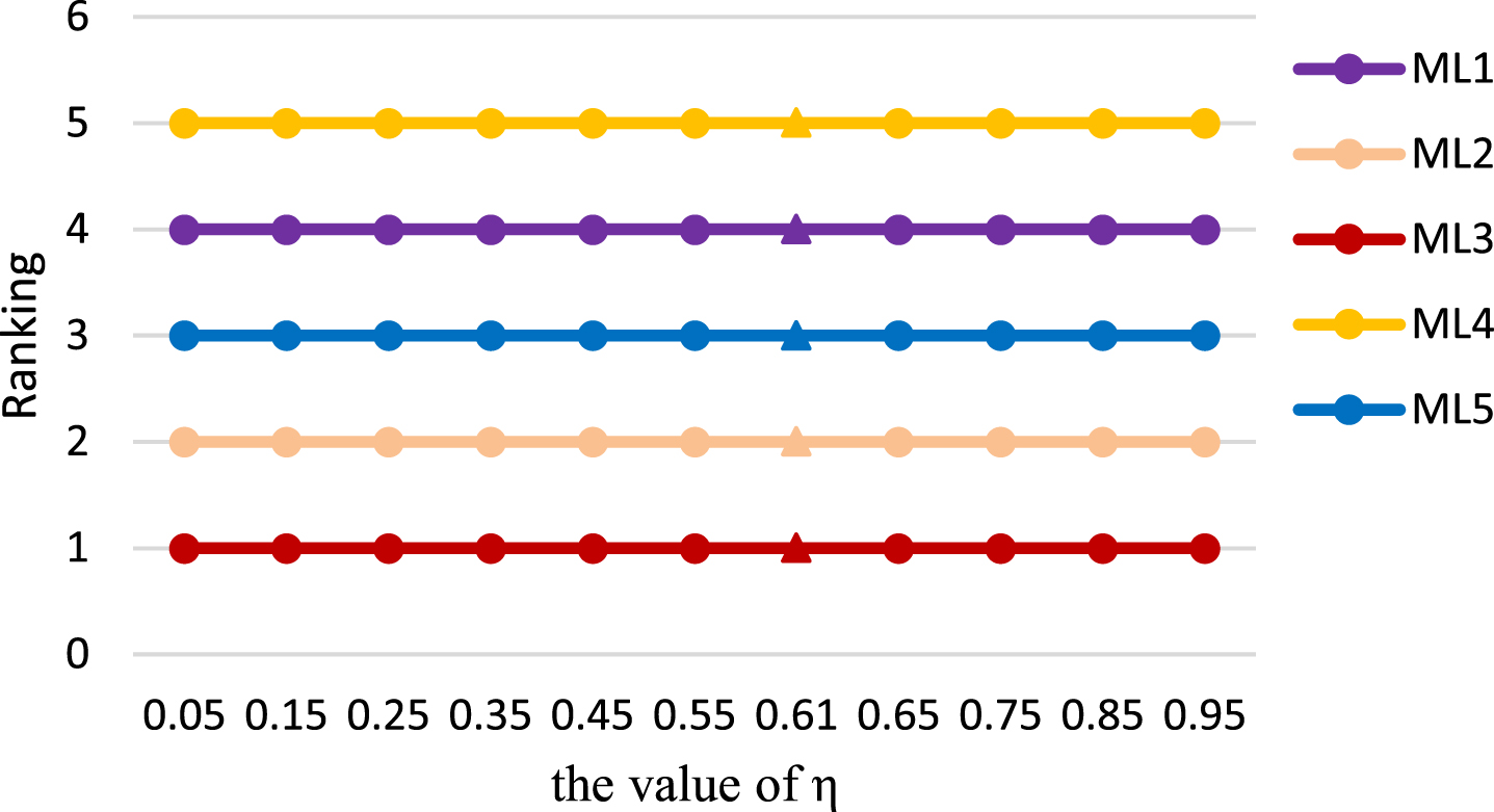
From the results of Table 4.22, Figs. 4.1 and 4.2, the results of IVIF-CPT-MABAC method will fluctuate to some extent with different value of η. With the value of η increase, the change trend of the total distance of all alternatives is to increase first and then decrease, where ML3 changes the most and ML4 changes the least. The order of the options remains the same, and the best and worst option is ML3 and ML4 respectively.
Fig. 4.1
The overall distance between different parameters η.
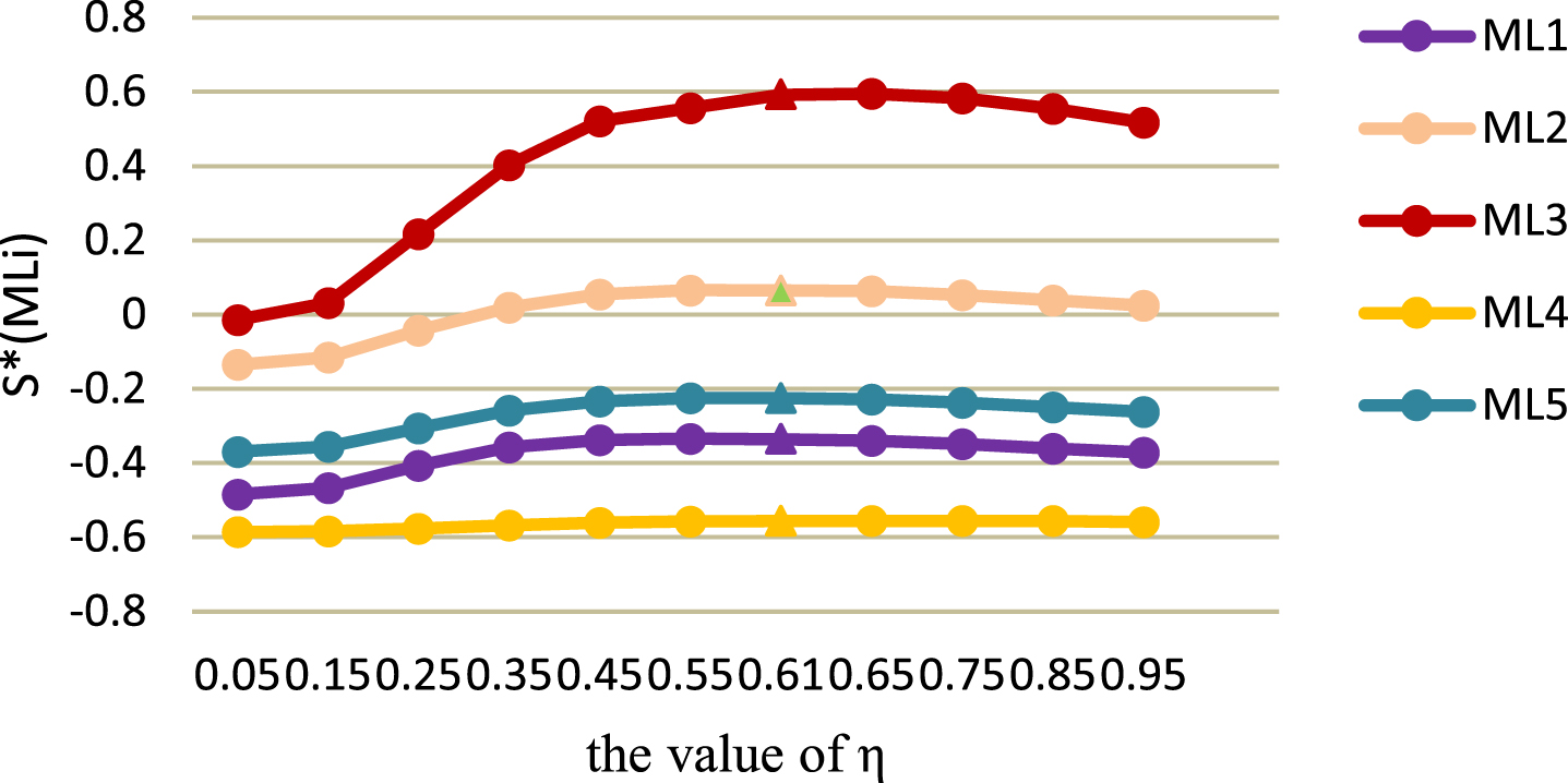
Fig. 4.2
The alternative ranking results of different parameters η.
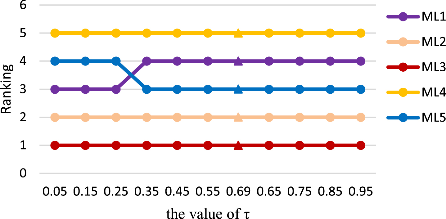
4.2.2The sensitivity analysis of parameter τ in value function
When η = 0.61 and the parameter in value function are constant, then the overall distance and ranking results of alternatives can be obtained by different value of parameter τ in weighting function in Table 4.23.
Table 4.23
The corresponding results of different value of parameter τ
| τ | ML1 | ML2 | ML3 | ML4 | ML5 | Ranking results | Optimal alternative |
| 0.69 | –0.336 | 0.065 | 0.592 | –0.556 | –0.225 | ML3 > ML2 > ML5 > ML1 > ML4 | ML3 |
| 0.05 | 0.148 | 0.200 | 0.606 | 0.030 | 0.143 | ML3 > ML2 > ML5 > ML1 > ML4 | ML3 |
| 0.15 | 0.114 | 0.192 | 0.605 | –0.027 | 0.101 | ML3 > ML2 > ML5 > ML1 > ML4 | ML3 |
| 0.25 | –0.032 | 0.156 | 0.599 | –0.240 | –0.051 | ML3 > ML2 > ML5 > ML1 > ML4 | ML3 |
| 0.35 | –0.183 | 0.117 | 0.593 | –0.430 | –0.175 | ML3 > ML2 > ML5 > ML1 > ML4 | ML3 |
| 0.45 | –0.282 | 0.088 | 0.591 | –0.534 | –0.234 | ML3 > ML2 > ML5 > ML1 > ML4 | ML3 |
| 0.55 | –0.329 | 0.072 | 0.591 | –0.570 | –0.246 | ML3 > ML2 > ML5 > ML1 > ML4 | ML3 |
| 0.65 | –0.339 | 0.066 | 0.592 | –0.565 | –0.234 | ML3 > ML2 > ML5 > ML1 > ML4 | ML3 |
| 0.75 | –0.326 | 0.066 | 0.593 | –0.538 | –0.210 | ML3 > ML2 > ML5 > ML1 > ML4 | ML3 |
| 0.85 | –0.300 | 0.071 | 0.595 | –0.499 | –0.181 | ML3 > ML2 > ML5 > ML1 > ML4 | ML3 |
| 0.95 | –0.267 | 0.079 | 0.597 | –0.456 | –0.152 | ML3 > ML2 > ML5 > ML1 > ML4 | ML3 |
From the results of Table 4.23, Figs. 4.3 and 4.4, the results of IVIF-CPT-MABAC method will fluctuate to some extent with different value of τ. With the value of τ increase, the change trend of the total distance of all alternatives is to decrease first and then increase, where ML3 changes the most and ML4 changes the least. Though the order of the options has a little difference when τ = 0.05, 0.15, 0.25, where ML3 changes the most and ML4 changes the least. The order of the options has little difference, and the best and worst option is ML3 and ML4 respectively.
Fig. 4.3
The overall distance of different parameter τ.
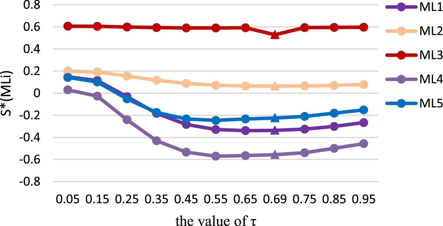
Fig. 4.4
The alternative ranking results of different parameters τ.
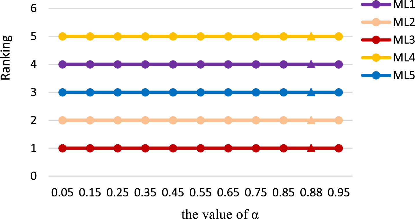
4.2.3The sensitivity analysis of parameter α in value function
When β = 0.88, ρ = 2.25 and the parameter in weighting function are constant, then the overall distance and ranking results of alternatives are shown in Table 4.24.
Table 4.24
The corresponding results of different value of parameters α
| α | ML1 | ML2 | ML3 | ML4 | ML5 | Ranking results | Optimal alternative |
| 0.88 | –0.336 | 0.065 | 0.592 | –0.556 | –0.225 | ML3 > ML2 > ML5 > ML1 > ML4 | ML3 |
| 0.05 | 0.011 | 0.540 | 1.066 | –0.315 | 0.100 | ML3 > ML2 > ML5 > ML1 > ML4 | ML3 |
| 0.15 | –0.056 | 0.441 | 0.977 | –0.378 | 0.034 | ML3 > ML2 > ML5 > ML1 > ML4 | ML3 |
| 0.25 | –0.115 | 0.359 | 0.902 | –0.427 | –0.023 | ML3 > ML2 > ML5 > ML1 > ML4 | ML3 |
| 0.35 | –0.165 | 0.289 | 0.836 | –0.464 | –0.070 | ML3 > ML2 > ML5 > ML1 > ML4 | ML3 |
| 0.45 | –0.208 | 0.231 | 0.779 | –0.492 | –0.110 | ML3 > ML2 > ML5 > ML1 > ML4 | ML3 |
| 0.55 | –0.246 | 0.182 | 0.728 | –0.514 | –0.145 | ML3 > ML2 > ML5 > ML1 > ML4 | ML3 |
| 0.65 | –0.278 | 0.140 | 0.682 | –0.531 | –0.174 | ML3 > ML2 > ML5 > ML1 > ML4 | ML3 |
| 0.75 | –0.306 | 0.104 | 0.640 | –0.544 | –0.198 | ML3 > ML2 > ML5 > ML1 > ML4 | ML3 |
| 0.85 | –0.330 | 0.074 | 0.603 | –0.554 | –0.220 | ML3 > ML2 > ML5 > ML1 > ML4 | ML3 |
| 0.95 | –0.350 | 0.047 | 0.569 | –0.561 | –0.238 | ML3 > ML2 > ML5 > ML1 > ML4 | ML3 |
From the results of Table 4.24, Figs. 4.5 and 4.6, the results of IVIF-CPT-MABAC method will fluctuate to some extent with different value of α. With the value of α increase, the change trend of the total distance of all alternatives is decrease. The order of the options remains constantly, and the best and worst option is ML3 and ML4 respectively.
Fig. 4.5
The overall distance of different parameters α.
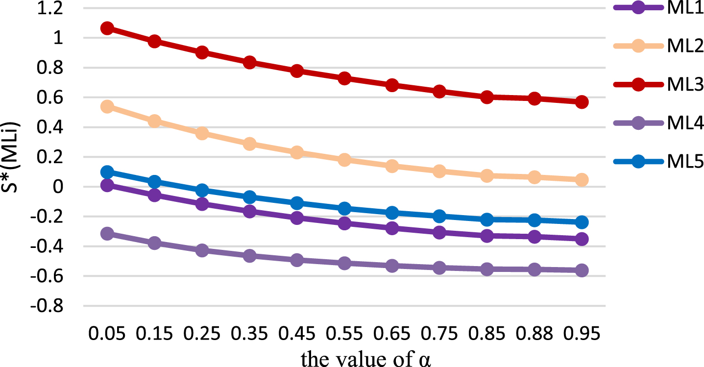
Fig. 4.6
The alternative ranking results of different parameters α.
4.2.4The sensitivity analysis of parameter β in value function
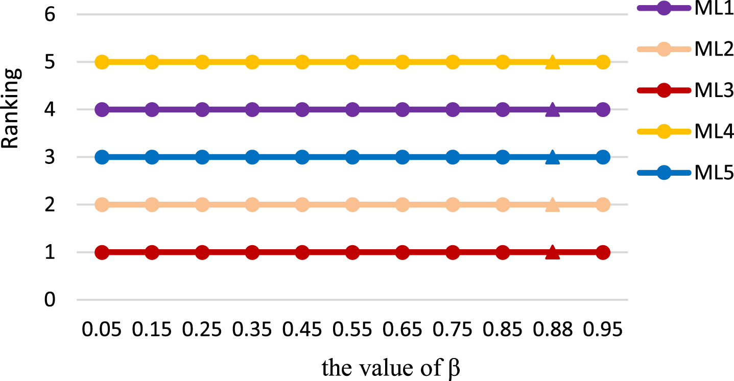
When α = 0.88, ρ = 2.25 and the parameter in weighting function are constant, and the overall distance and ranking results of alternatives with different value of parameter β are shown in Table 4.25.
Table 4.25
The corresponding results of different value of parameter β
| β | ML1 | ML2 | ML3 | ML4 | ML5 | Ranking results | Optimal alternative |
| 0.88 | –0.336 | 0.065 | 0.592 | –0.556 | –0.225 | ML3 > ML2 > ML5 > ML1 > ML4 | ML3 |
| 0.05 | –1.489 | –0.994 | 0.267 | –1.989 | –1.450 | ML3 > ML2 > ML5 > ML1 > ML4 | ML3 |
| 0.15 | –1.251 | –0.718 | 0.375 | –1.690 | -1.148 | ML3 > ML2 > ML5 > ML1 > ML4 | ML3 |
| 0.25 | –1.051 | –0.506 | 0.449 | –1.440 | –0.915 | ML3 > ML2 > ML5 > ML1 > ML4 | ML3 |
| 0.35 | –0.883 | –0.343 | 0.499 | –1.230 | –0.733 | ML3 > ML2 > ML5 > ML1 > ML4 | ML3 |
| 0.45 | –0.741 | –0.217 | 0.534 | –1.054 | –0.589 | ML3 > ML2 > ML5 > ML1 > ML4 | ML3 |
| 0.55 | –0.621 | –0.121 | 0.557 | –0.905 | –0.474 | ML3 > ML2 > ML5 > ML1 > ML4 | ML3 |
| 0.65 | –0.518 | –0.047 | 0.573 | –0.779 | –0.381 | ML3 > ML2 > ML5 > ML1 > ML4 | ML3 |
| 0.75 | –0.431 | 0.010 | 0.583 | –0.672 | –0.305 | ML3 > ML2 > ML5 > ML1 > ML4 | ML3 |
| 0.85 | –0.357 | 0.054 | 0.591 | –0.581 | –0.242 | ML3 > ML2 > ML5 > ML1 > ML4 | ML3 |
| 0.95 | –0.292 | 0.088 | 0.596 | –0.503 | –0.190 | ML3 > ML2 > ML5 > ML1 > ML4 | ML3 |
From the results of Table 4.25, Figs. 4.7 and 4.8, the results of IVIF-CPT-MABAC method will fluctuate to some extent with different value of β. With the value of β increase, the change trend of the total distance of all alternatives is increase. The order of the options remains constantly, and the best and worst option is ML3 and ML4 respectively.
Fig. 4.7
The overall distance of different value of parameter β.
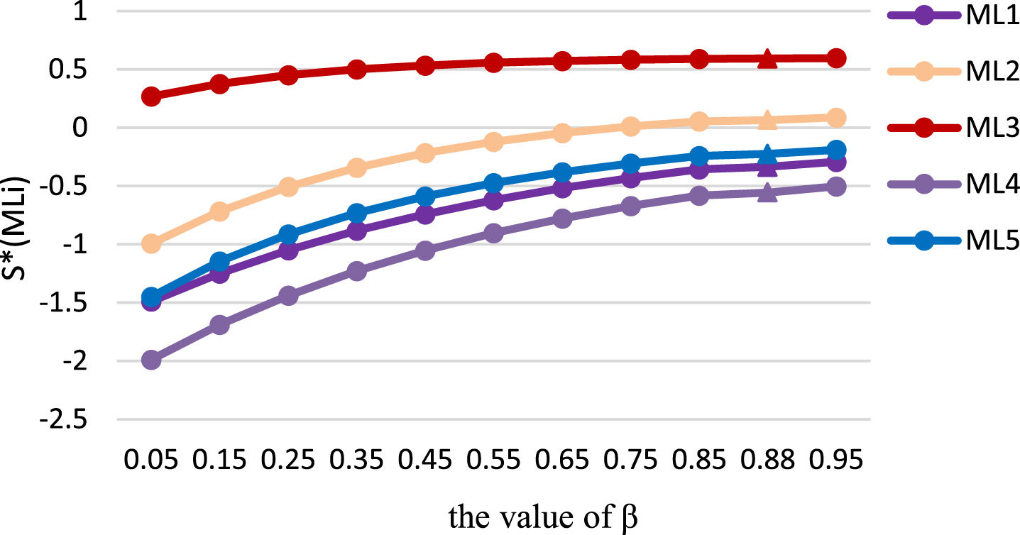
Fig. 4.8
The alternative ranking results of different parameters β.
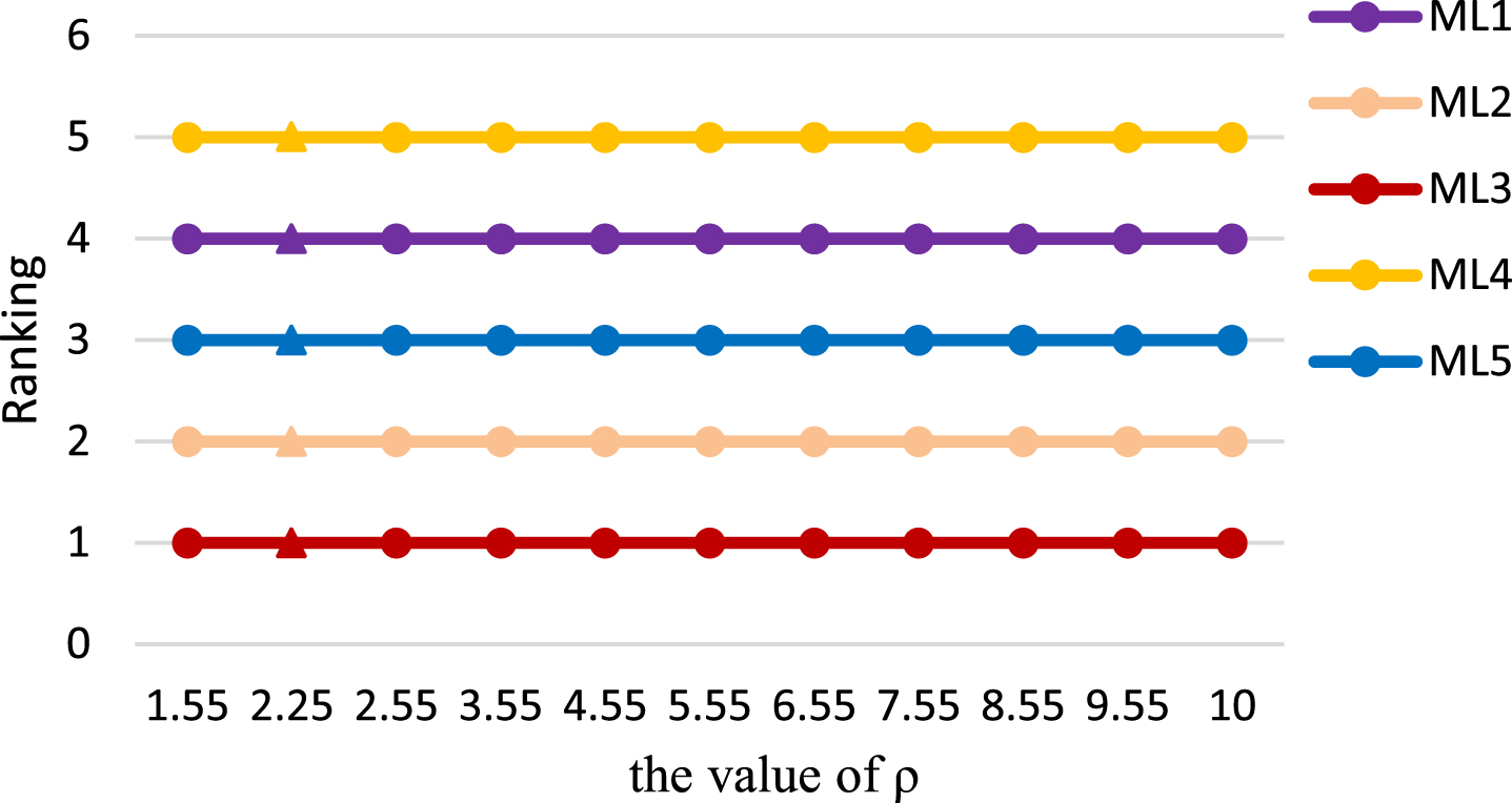
4.2.5The sensitivity analysis of parameter ρ in value function
When α = 0.88, β = 0.88 and the parameter in weighting function are constant, and the overall distance and ranking results of alternatives with different value of parameter ρ are shown in Table 4.26.
Table 4.26
The corresponding results of different value of parameter ρ
| ρ | ML1 | ML2 | ML3 | ML4 | ML5 | Ranking results | Optimal alternative |
| 2.25 | –0.336 | 0.065 | 0.592 | –0.556 | –0.225 | ML3 > ML2 > ML5 > ML1 > ML4 | ML3 |
| 1.55 | –0.186 | 0.107 | 0.597 | –0.374 | –0.111 | ML3 > ML2 > ML5 > ML1 > ML4 | ML3 |
| 2.55 | –0.401 | 0.047 | 0.591 | –0.634 | –0.275 | ML3 > ML2 > ML5 > ML1 > ML4 | ML3 |
| 3.55 | -0.616 | –0.013 | 0.584 | –0.895 | –0.439 | ML3 > ML2 > ML5 > ML1 > ML4 | ML3 |
| 4.55 | –0.831 | –0.073 | 0.578 | –1.155 | –0.603 | ML3 > ML2 > ML5 > ML1 > ML4 | ML3 |
| 5.55 | –1.047 | –0.132 | 0.572 | –1.416 | –0.767 | ML3 > ML2 > ML5 > ML1 > ML4 | ML3 |
| 6.55 | –1.262 | –0.192 | 0.566 | –1.676 | –0.931 | ML3 > ML2 > ML5 > ML1 > ML4 | ML3 |
| 7.55 | –1.477 | –0.252 | 0.560 | –1.937 | –1.094 | ML3 > ML2 > ML5 > ML1 > ML4 | ML3 |
| 8.55 | –1.693 | –0.312 | 0.553 | –2.197 | –1.258 | ML3 > ML2 > ML5 > ML1 > ML4 | ML3 |
| 9.55 | –1.908 | –0.372 | 0.547 | –2.457 | –1.422 | ML3 > ML2 > ML5 > ML1 > ML4 | ML3 |
| 10.00 | –2.005 | –0.399 | 0.545 | –2.575 | –1.496 | ML3 > ML2 > ML5 > ML1 > ML4 | ML3 |
From the results of Table 4.26, Figs. 4.9 and 4.10, the results of IVIF-CPT-MABAC method will fluctuate to some extent with different value of ρ. With the value of ρ increase, the change trend of the total distance of all alternatives is decrease, and alternative ML4 decreases the most specially. The order of the options remains constantly, and the best and worst option is ML3 and ML4 respectively.
Fig. 4.9
The overall distance of different value of parameter ρ.
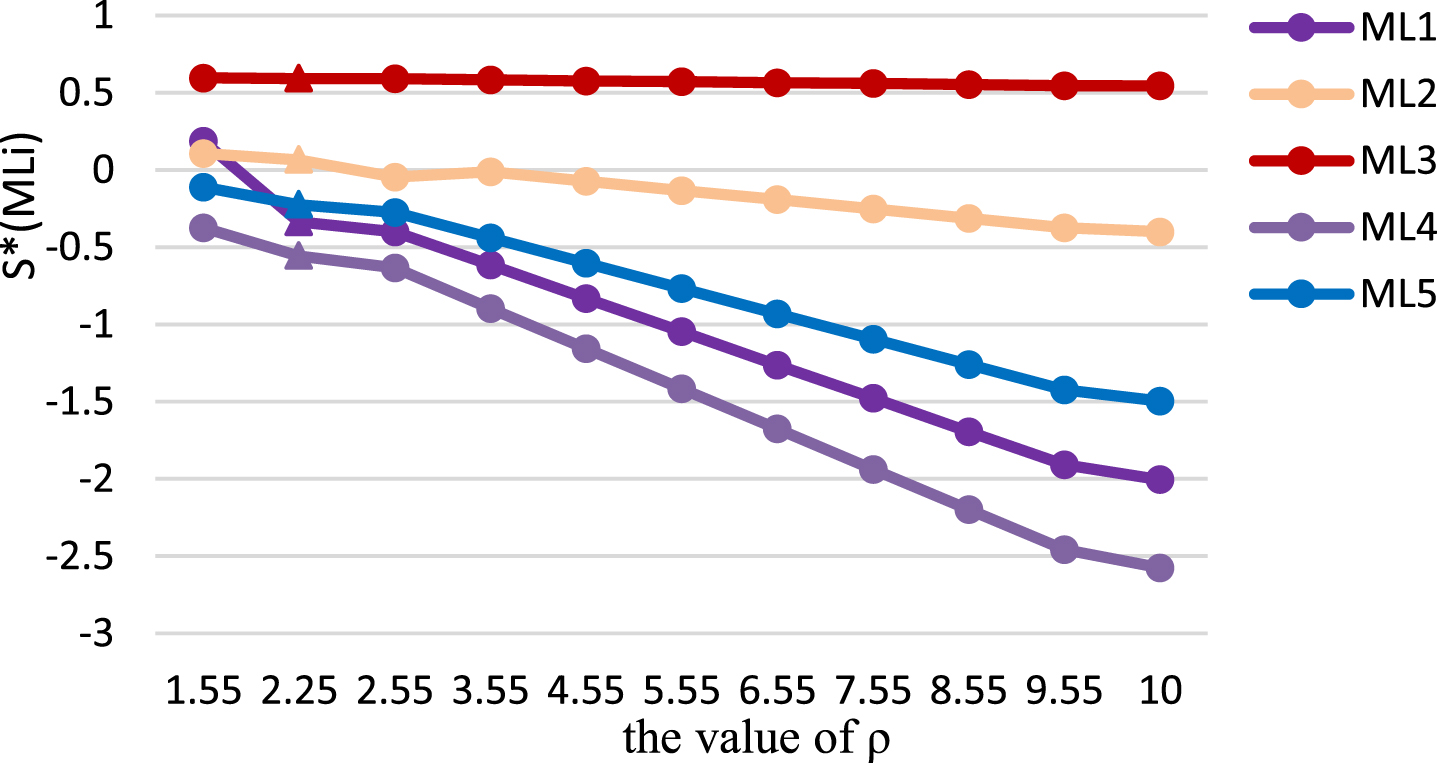
Fig. 4.10
The alternative ranking results of different parameters ρ.
According to the above observation and analysis results, although the change of parameters in the weight function and value function will cause certain fluctuations to the calculation results of the model, it will not change the optimal solution and the worst solution in the decision results. Therefore, the IVIF-CPT-MABAC method is robust and effective. Meanwhile, when DMs’ psychological preference is not obvious, the difference between the superior and inferior alternatives does not change much; when DM’s psychological preference is obvious, the difference between the superior and inferior alternatives change much. Thus, the IVIF-CPT-MABAC method in this paper is more in line with the realistic decision environment.
4.3Comparison analysis
In this section, in order to prove the effectiveness of the IVIF-CPT-MABAC method, we compare the IVIF-CPT-MABAC method with several classical MADM method based on the same initial matrix. The classical method is listed as follows: IVIFWA operator [17], IVIFWG operator [17], IVIF-TAXONOMY method [78], IVIF-WASPAS method [79], IVIF-TOPSIS method [80] and IVIF-CPT-TODIM method [81]. The specific calculation results are shown in Table 4.27 to 4.33.
Table 4.27
The calculation results of IVIFWA operator
| Alternative | IVIFWA | SF (MLr) | AF (MLr) | Ranking results |
| ML1 | 〈 [0.461, 0.560] , [0.276, 0.334]〉 | 0.205 | 0.816 | 4 |
| ML2 | 〈 [0.551, 0.649] , [0.188, 0.246]〉 | 0.384 | 0.817 | 2 |
| ML3 | 〈 [1.000, 1.000] , [0.000, 0.000]〉 | 1.000 | 1.000 | 1 |
| ML4 | 〈 [0.427, 0.536] , [0.259, 0.334]〉 | 0.185 | 0.778 | 5 |
| ML5 | 〈 [0.533, 0.648] , [0.178, 0.255]〉 | 0.374 | 0.807 | 3 |
Table 4.28
The calculation results of IVIFWG operator
| Alternative | IVIFWG | SF (MLr) | AF (MLr) | Ranking results |
| ML1 | 〈 [0.401, 0 . 497] , [0 . 324, 0.391]〉 | 0.092 | 0.807 | 3 |
| ML2 | 〈 [0.534, 0.626] , [0 . 212, 0.272]〉 | 0.338 | 0.822 | 2 |
| ML3 | 〈 [0 . 699, 0 . 771] , [0 . 117, 0 . 171]〉 | 0.591 | 0.879 | 1 |
| ML4 | 〈 [0 . 000, 0 . 367] , [0 . 414, 0 . 480]〉 | –0.263 | 0.630 | 5 |
| ML5 | 〈 [0 . 000, 0 . 479] , [0 . 323, 0 . 386]〉 | –0.115 | 0.594 | 4 |
Table 4.29
The calculation results of IVIF-Taxonomy
| Alternative | Fi (MLi) | Ranking results |
| ML1 | 0.472 | 3 |
| ML2 | 0.538 | 2 |
| ML3 | 0.947 | 1 |
| ML4 | 0.468 | 4 |
| ML5 | 0.178 | 5 |
Table 4.30
The corresponding calculation results of IVIF-WASPAS
| Alternative | SF (MLi) | AF (MLi) | Ranking |
| ML1 | 0.204 | 0.816 | 4 |
| ML2 | 0.346 | 0.812 | 2 |
| ML3 | 1 | 1 | 1 |
| ML4 | 0.077 | 0.764 | 5 |
| ML5 | 0.217 | 0.793 | 3 |
Table 4.31
The corresponding calculation results of IVIF-TOPSIS
| Alternative |
|
| Ci | Ranking |
| ML1 | 0.071 | 0.031 | 0.303 | 4 |
| ML2 | 0.051 | 0.051 | 0.502 | 2 |
| ML3 | 0.007 | 0.112 | 0.942 | 1 |
| ML4 | 0.084 | 0.035 | 0.294 | 5 |
| ML5 | 0.064 | 0.054 | 0.456 | 3 |
Table 4.32
The original attribute weight ϖj
| Original | MT1 | MT2 | MT3 | MT4 | MT5 | MT6 |
| attribute | ||||||
| weight | ||||||
| ϖj | 0.172 | 0.162 | 0.174 | 0.163 | 0.159 | 0.171 |
Table 4.33
The corresponding calculation results of IVIF-CPT-TODIM
| Alternative | Ω (MLr) | ℏ (MLr) | Ranking |
| ML1 | –49.850 | 0.358 | 3 |
| ML2 | –28.390 | 0.696 | 2 |
| ML3 | –9.075 | 1 | 1 |
| ML4 | –72.635 | 0 | 5 |
| ML5 | –62.689 | 0.156 | 4 |
4.3.1Compare with IVIFWA operator [17]
Substitute the Table 4.7 to Table 4.11, weighting vector of experts ϑ = (ϑ1, ϑ2, ⋯ , ϑ5) = (0.27, 0.16, 0.23, 0.16, 0.18) and original attribute weight ω = (ω1, ω2, ⋯ , ω6) = (0.243, 0.113, 0.283, 0 . 043, 0 . 0290 . 288) into Equation (2.15), and get the calculation results in Table 4.27.
4.3.2Compare with IVIFWG operator [17]
Substitute the Table 4.7 to Table 4.11, weighting vector of experts ϑ = (ϑ1, ϑ2, ⋯ , ϑ5) = (0.27, 0.16, 0.23, 0.16, 0.18) and original attribute weight ω = (ω1, ω2, ⋯ , ω6) = (0.243, 0.113, 0.283, 0 . 043, 0 . 0290 . 288) into Equation (2.16), and get the calculation results in Table 4.28.
The IVIFWA and IVIFWG operator are the classical MADM methods. Tables 4.27 and 4.28 show the ranking decision results of IVIFWA operator is ML3 > ML2 > ML5 > ML1 > ML4. The decision result is slightly different from the results of improved MABAC method, but it does not affect the selection of the optimal scheme and the worst scheme, so the IVIF-CPT-MABAC method in this paper is effective.
4.3.3Compare with IVIF-Taxonomy method [78]
The IVIF-Taxonomy method mainly classifies and compares alternatives and uses mean and standard deviation to determine the development value of alternatives. The larger the development value, the better the alternative. Substitute the Tables 4.7 to 4.11, weighting vector of experts ϑ = (ϑ1, ϑ2, ⋯ , ϑ5) = (0.27, 0.16, 0.23, 0.16, 0.18) and original attribute weight ω = (ω1, ω2, ⋯ , ω6) = (0.243, 0.113, 0.283, 0 . 043, 0 . 0290 . 288) into Equation (2.16), and get the calculation results in Table 4.29.
The main steps are as follows:
Step 1. Obtain the composite matrix of distance mpq using Equation (4.1)
(4.1)
Step 2. The alternatives are homogenized by formula (4.2)
(4.2)
Step 3. Determine the alternative and development model using Equation (4.3), and select the optimal alternative in Table 4.29 using Equation (4.4) and Equation (4.5).
(4.3)
(4.4)
(4.5)
Table 4.29 shows that the decision result of IVIF-Taxonomy method is ML3 > ML2 > ML1 > ML4 > ML5. The result shows that the optimal alternative is still ML3, and the IVIF-CPT-MABAC method is effective.
4.3.4Compare with IVIF-WASPAS [79]
The IVIF-WASPAS method, combining with the weighted sum model (WSM) and weighted product model (WPM), ranks the alternative by determining the relative importance of each attribute. the larger the relative importance, the better the alternative. The calculation results obtained by following the main steps are shown in Table 4.30
The specific steps are as follows:
Step 1. Determine the normalize decision matrix
(4.6)
(4.7)
Step 2. Obtain the sum and product of relative importance using Equation (4.8) and Equation (4.9).
(4.8)
(4.9)
Step 3. Calculate the Joint generalized criterion values
(4.10)
(4.11)
(4.12)
Table 4.30 shows that the decision result of IVIF-WASPAS method is ML3 > ML2 > ML5 > ML1 > ML4. The result shows that the optimal alternative is still ML3, and the IVIF-CPT-MABAC method is effective.
4.3.5Compare with IVIF-TOPSIS method [80]
IVIF-TOPSIS method mainly calculates the distance between alternative solutions and positive and negative ideal solutions (PIS and NIS). The smaller the distance between alternative solutions and positive ideal solutions, the larger the distance between alternative solutions and negative ideal solutions, the better the solution. The sorting results in Table 4.31 are obtained by the following steps.
The main steps are as follows:
Step 1. Determine the IVIF PIS
(4.13)
(4.14)
Step 2. The distance between each alternative between IVIF PIS and IVIF NIS using Equation (4.15) and Equation (4.16).
(4.15)
(4.16)
Step 3. Calculate the relative proximity degree between each alternative between each alternative and IVIF PIS. The larger the relative proximity degree, the better the alternative.
(4.17)
Table 4.30 shows that the decision result of IVIF-TOPSIS method is ML3 > ML2 > ML5 > ML1 > ML4. The result shows that the optimal alternative is still ML3, and the IVIF-CPT-MABAC method is effective.
4.3.4Compare with IVIF-CPT-TODIM method [81]
IVIF-CPT-TODIM method mainly refers to each other through pairwise alternatives, and uses the overall value to measure the superiority of each alternative compared with other alternatives. The greater the superiority, the better the solution. The main steps are listed as follows:
Step 1. Obtain the original attribute weight using entropy method in Table 4.32.
(4.18)
(4.19)
(4.20)
Step 2. Calculate the percentage weight between MLr and MLi using Equation (4.21) and (4.22). (η = 0.61, τ = 0.69)
(4.21)
(4.22)
Step 3. Calculate the Proportional prospect advantage of between MLr and MLi under attribute MTj (α = 0.88, β = 0.88, ρ = 2.25).
(4.23)
(4.24)
Step 4. Calculate the prospect value of MLr (r = 1, 2, ⋯ , n) using Equation (4.26)
(4.25)
(4.26)
Step 5. Rank the alternatives with the calculation results in Step 4. The larger the value of ℏ (MLr), the better the alternative.
According to Table 4.33, we observe that the decision results of IVIF-CPT-TODIM method and the decision results of improved MABAC method in this paper exchange the order of ML1 and ML5, but it does not affect the selection of the optimal scheme and the worst scheme. Therefore, the IVIF-CPT-MABAC method in this manuscript is effective.
Fig. 4.12
The ranking results of different methods.
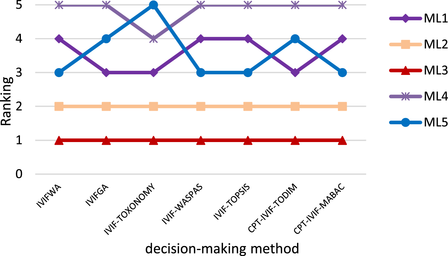
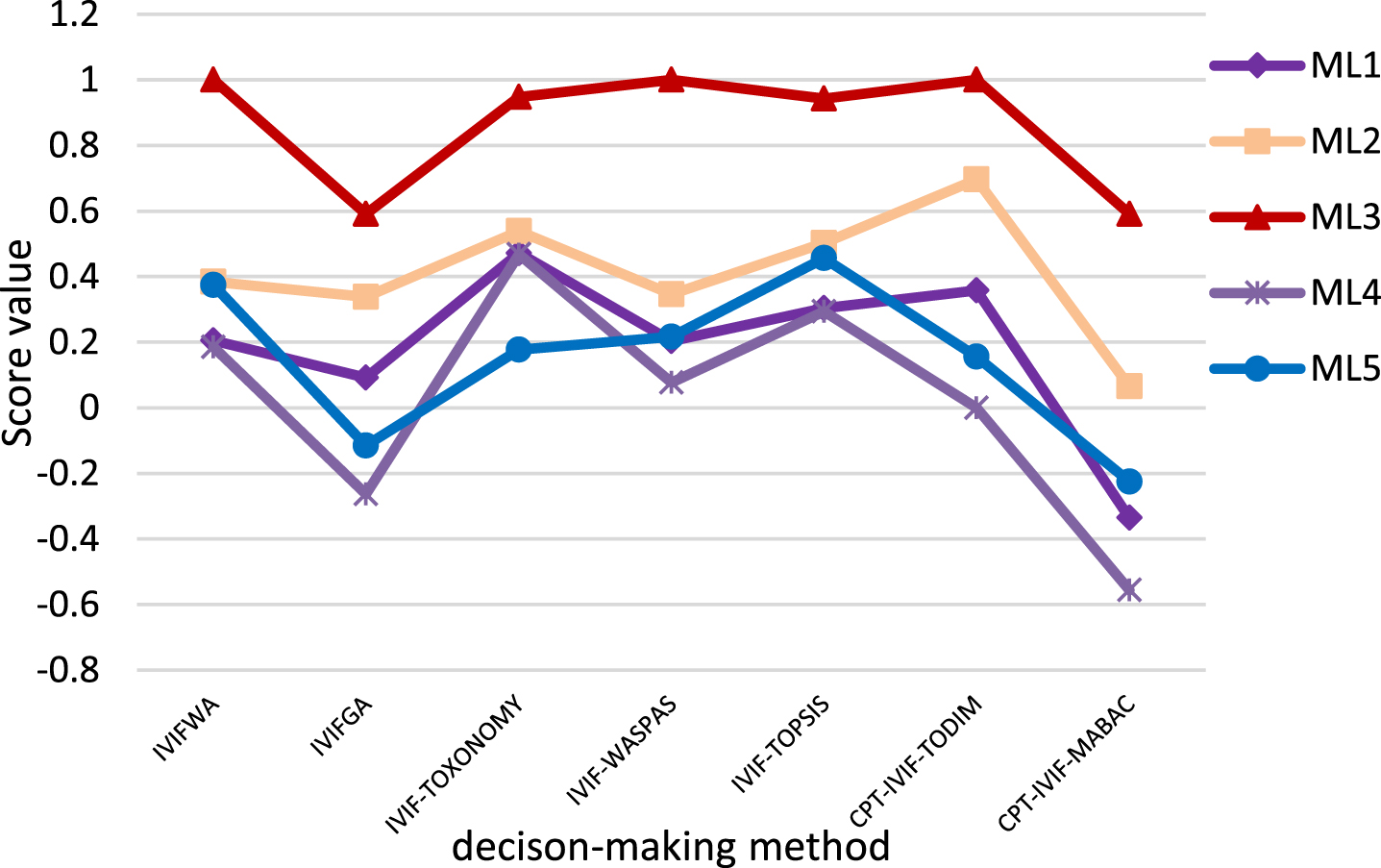
4.3.7Comprehensive analysis
According to the ranking of the five schemes calculated by the six decision-making methods shows in Table 4.34, Figs. 4.10 and 4.11, we see that although the ranking of the five options is slightly different, the best scheme is always ML3. Therefore, we can conclude that based on the same initial matrix of this paper, the extended method in this paper is effective. In the same fuzzy environment, different MAGDM methods have their own advantages. IVIFWA operator pays more attention to the overall balance while IVIFWG operator focus on unit, and they have a common shortcoming, that is, they can’t evaluate extreme values. IVIF-TAXONOMY method has less possibility of information distortion in the process of information aggregation. IVIF-WASPAS method is proposed base on IVIFWA and IVIFWG, so this method has the same weakness as them. The IVIF-TOPSIS method and IVIF-CPT-TODIM method have simple decision-making principles and use distance matrix to make decisions, but they are only suitable for conservative decision makers. However, compared with the above decision-making methods, the IVIF-CPT-MABAC method constructed in this paper not only considers the influence of the decision-maker’s psychological factors, but also improves the decision-making method through the cumulative prospect function, so the algorithm logic in this paper is closer to the real decision-making environment. In addition, the improved method proposed in the study better handles the MAGDM problems with IVIF information and attribute indicators with local advantages in the decision-making process, and has strong practicability.
Table 4.34
The ranking results of different methods
| Decision-making methods | Alternative order | The optimum | The worst |
| solution | solution | ||
| IVIFWA | ML3 > ML2 > ML5 > ML1 > ML4 | ML3 | ML4 |
| IVIFWG | ML3 > ML2 > ML1 > ML5 > ML4 | ML3 | ML4 |
| IVIF-TOXONOMY | ML3 > ML2 > ML1 > ML4 > ML5 | ML3 | ML5 |
| IVIF-WASPAS | ML3 > ML2 > ML5 > ML1 > ML4 | ML3 | ML4 |
| IVIF-TOPSIS | ML3 > ML2 > ML5 > ML1 > ML4 | ML3 | ML4 |
| IVIF-CPT-TODIM | ML3 > ML2 > ML1 > ML5 > ML4 | ML3 | ML4 |
| IVIF-CPT-MABAC | ML3 > ML2 > ML5 > ML1 > ML4 | ML3 | ML4 |
Fig. 4.11
The score value of different methods.
5Conclusion
In this paper, we study the MABAC method combined with CPT to solve MAGDM problem in the interval intuitionistic fuzzy environment. Firstly, we introduce the basic definition of IVIFS, the comparison formula, the related aggregation operator, and the mixing distance of Hamming and Hausdorff. We know that the calculation formula of MABAC method is simple, the result is stable, the hidden gains and losses are considered, and it is easy to combine with other methods for decision analysis. This method evaluates the alternatives by defining the closeness between the possible solution and the BAA. if the closeness degree is larger, then the alternative is better. However, the calculation of the BAA is greatly affected by the extreme value, so it is more suitable for the situation where the attribute index has local advantages. Therefore, CRITIC method, which comprehensively uses correlation coefficient and standard deviation principle in statistics to determine attribute weight, plays an important role in the improved MABAC method, that is, the larger the standard deviation of indicators with local advantages, the greater the impact of volatility on the overall evaluation value, the greater the weight given to the index, which is just suitable for the decision-making characteristics of MABAC method. Then, we not only integrate the CPT that represents the decision-maker’s risk preference into the classic MABAC decision method, but also use IVIFNs to represent the evaluation value of attributes to jointly construct the IVIF-CPT-MABAC method, so as to retain the collected expert evaluation opinions more clearly and completely, making the decision results more accurate and efficient. Next, we apply the IVIF-CPT-MABAC method to the selection of green suppliers to verify the feasibility of the improved method in this paper. Besides, the sensitivity analysis conducted by controlling the individual changes of each parameter in the model can be seen as simulating the impact of the psychological changes of the decision-maker on the decision results to verify the stability of the construction method in this paper. Finally, compared with other six classical MAGDM methods to verify the effectiveness of the method created in this paper in solving uncertain decision problems.
In future research, we will focus on building new models and functions to determine attribute weights so that attribute weights can dynamically change with data. At the same time, we will explore more applications of the new method in this paper and other more effective solutions of MAGDM. At the same time, with the development of network technology [82], a large number of decision-making methods in network form have emerged, such as microblog, WeChat, QQ and other online voting forms, so DMs are involved in different decision-making complexes [83]. In theory, facing such complex decision-making, we can also expand the research results of this paper to the research direction of complex decision-making with the times.
Acknowledgments
The work was supported by the National Social Science Foundation of China under Grant No. 21XJY003 and Sichuan Province Social Development Key R&D Projects under Grant No. 2023YFS0375.
Compliance with ethical standards
Ethical approval
This article does not contain any studies with human participants or animals performed by any of the authors.
Conflict of interest
The authors declare that they have no conflict of interest.
References
[1] | Zadeh L.A. , Fuzzy sets, Information and Control 8: ((1965) ), 338–353. |
[2] | Huang Y.B. and Jiang W. , Extension of TOPSIS method and its application in investment, Arabian Journal for Science and Engineering 43: ((2018) ), 693–705. |
[3] | Wang Y.N. , Zhang Z. and Sun H. , Assessing customer satisfaction of urban rail transit network in Tianjin based on intuitionistic fuzzy group decision model, Discrete Dynamics in Nature and Society 2018: ((2018) ), 4205136. |
[4] | Torra V. , Hesitant fuzzy sets, International Journal of Intelligent Systems 25: ((2010) ), 529–539. |
[5] | Xu Z.S. and Yager R.R. , Some geometric aggregation operators based on intuitionistic fuzzy sets, International Journal of General Systems 35: ((2006) ), 417–433. |
[6] | Xu Z.S. , Intuitionistic fuzzy aggregation operators, Ieee Transactions on Fuzzy Systems 15: ((2007) ), 1179–1187. |
[7] | Xu Z.S. , Dynamic intuitionistic fuzzy multi-attribute decision making (vol 48, pg 246, 2008), International Journal of Approximate Reasoning 51: ((2009) ), 162–164. |
[8] | Atanassov K.T. and Gargov G. , Interval valued intuitionistic fuzzy sets, Fuzzy Sets and Systems 31: ((1989) ), 343–349. |
[9] | Atanassov K.T. , Operators over interval valued intuitionistic fuzzy sets, Fuzzy Sets and Systems 64: ((1994) ), 159–174. |
[10] | Chen S.M. and Tsai C.A. , Multiattribute decision making using novel score function of interval-valued intuitionistic fuzzy values and the means and the variances of score matrices, Information Sciences 577: ((2021) ), 748–768. |
[11] | Chen S.M. and Yu S.H. , Multiattribute decision making based on novel score function and the power operator of interval-valued intuitionistic fuzzy values, Information Sciences 606: ((2022) ), 763–785. |
[12] | Haktanir E. and Kahraman C. , New product design using chebyshev’s inequality based interval-valued intuitionistic Z-fuzzy QFD method, Informatica (2022), 1–33. |
[13] | Salimian S. , Mousavi S.M. and Antucheviciene J. , Evaluation of infrastructure projects by a decision model based on RPR, MABAC, and WASPAS methods with interval-valued intuitionistic fuzzy sets, International Journal of Strategic Property Management 6: ((2022) ), 106–118. |
[14] | Wang F. and Wan S.P. , A comprehensive group decision-making method with interval-valued intuitionistic fuzzy preference relations, Soft Computing 25: ((2021) ), 343–362. |
[15] | Mondal T.K. and Samanta S.K. , Topology of interval-valued intuitionistic fuzzy sets, Fuzzy Sets Syst 119: ((2001) ), 483–494. |
[16] | Grzegorzewski P. , Distances between intuitionistic fuzzy sets and/or interval-valued fuzzy sets based on the Hausdorff metric, Fuzzy Sets and Systems 148: ((2004) ), 319–328. |
[17] | Xu Z.S. , Methods for aggregating interval-valued intuitionistic fuzzy information and their application to decision making, Control and Decision 22: ((2007) ), 215–219. |
[18] | Zhang H.Y. , Dong M.G. , Zhang W.X. and Song X.X. , Inclusion measure and similarity measure of intuitionistic and interval-valued fuzzy sets, in: 2007 International Conference on Intelligent Systems and Knowledge Engineering, Atlantis Press, Southwest Jiaotong Univ, Chengdu, PEOPLES R CHINA, 2007. |
[19] | Senapati T. , Chen G.Y. , Mesiar R. and Yager R.R. , Novel Aczel-Alsina operations-based interval-valued intuitionistic fuzzy aggregation operators and their applications in multiple attribute decision-making process, International Journal of Intelligent Systems 37: ((2022) ), 5059–5081. |
[20] | Hayat K. , Tariq Z. , Lughofer E. and Aslam M.F. , New aggregation operators on group-based generalized intuitionistic fuzzy soft sets, Soft Computing 25: ((2021) ), 13353–13364. |
[21] | Karaaslan F. , Another view of aggregation operators on group-based generalized intuitionistic fuzzy soft sets: multi-attribute decision making methods, Symmetry 10: ((2018) ). |
[22] | Hayat K. , Ali M.I. , Alcantud J.C.R. , Cao B.Y. and Tariq K. , Best concept selection in design process: An application of generalized intuitionistic fuzzy soft sets, Journal of Intelligent and Fuzzy Systems, (2018). |
[23] | Hayat K. , Ali M.I. , Karaaslan F. , Cao B.Y. and Shah M. , Design concept evaluation using soft sets based on acceptable and satisfactory levels: an integrated TOPSIS and Shannon entropy, Soft Computing 24: ((2020) ), 2229–2263. |
[24] | Hayat K. , Raja M.S. , Lughofer E. and Yaqoob N. , New group-based generalized interval-valued q-rung orthopair fuzzy soft aggregation operators and their applications in sports decision-making problems, Computational and Applied Mathematics 42: ((2022) ), 4. |
[25] | Yang X.P. , Hayat K. , Raja M.S. , Yaqoob N. and Jana C. , Aggregation and interaction aggregation soft operators on interval-valued q-rung orthopair fuzzy soft environment and application in automation company evaluation, IEEE Access 10: ((2022) ), 91424–91443. |
[26] | Wei G.W. and Wang X.R. , TOPSIS method for intervalvalued intuitionistic fuzzy multiple attribute decision making, in: Conference on Systems Science, Management Science and System Dynamics, System Dynamics Soc, Shanghai, PEOPLES R CHINA, 2007, pp. 2243–2249. |
[27] | Wei G.W. and Lan G. , Grey relational analysis method for interval-valued intuitionistic fuzzy multiple attribute decision making, in: in: 2008 Fifth International Conference on Fuzzy Systems and Knowledge Discovery, 2008, pp. 291–295. |
[28] | Zhang H.B. and Wang L. , The service quality evaluation of agricultural e-commerce eased on interval-valued intuitionistic fuzzy GRA method, Journal of Mathematics 2022: ((2022) ), 1–10. |
[29] | Xu X. , Wang W.Z. and Wang Z.J. , Maximizing deviation method for interval-valued intuitionistic fuzzy multiattribute decision making, in: 3rd International Conference on Computer Science and Education, Xiamen Univ Press, Kaifeng, PEOPLES R CHINA, 2008, pp. 1087–1092. |
[30] | Park J.H. , Cho H.J. and Kwun Y.C. , Extension of the VIKOR method for group decision making with interval-valued intuitionistic fuzzy information, Fuzzy Optimization and Decision Making 10: ((2011) ), 233–253. |
[31] | Salimian S. , Mousavi S.M. and Antucheviciene J. , An interval-valued intuitionistic fuzzy model based on extended VIKOR and MARCOS for sustainable supplier selection in organ transplantation networks for healthcare devices, Sustainability 14: ((2022) ), 3795. |
[32] | Xue Y.X. , You J.X. , Lai X.D. and Liu H.C. , An interval-valued intuitionistic fuzzy MABAC approach for material selection with incomplete weight information, Applied Soft Computing 38: ((2016) ), 703–713. |
[33] | Kabak Ö. and Ruan D. , A comparison study of fuzzy MADM methods in nuclear safeguards evaluation, Journal of Global Optimization 51: ((2011) ), 209–226. |
[34] | Yoon K.P. and Hwang C.-L. , Multiple attribute decision making: an introduction, Sage publications, 1995. |
[35] | Jie L. , Zhang G. , Da R. and Wu F. , Multi-objective group decision making: methods, software and applications, Social Science Electronic Publishing 28: ((2007) ), 144. |
[36] | Liang W.Z. , Zhao G.Y. , Wu H. and Dai B. , Risk assessment of rockburst via an extended MABAC method under fuzzy environment, Tunnelling and Underground Space Technology 83: ((2019) ), 533–544. |
[37] | Xian S.D. , Wan W.H. and Yang Z.J. , Interval-valued Pythagorean fuzzy linguistic TODIM based on PCA and its application for emergency decision, International Journal of Intelligent Systems 35: ((2020) ), 2049–2086. |
[38] | Chen S.M. and Liao W.T. , Multiple attribute decision making using Beta distribution of intervals, expected values of intervals, and new score function of interval-valued intuitionistic fuzzy values, Information Sciences 579: ((2021) ), 863–887. |
[39] | Chen S.M. and Tsai C.A. , Multiattribute decision making using novel score function of interval-valued intuitionistic fuzzy values and the means and the variances of score matrices, Information Sciences 577: ((2021) ), 748–768. |
[40] | Kahraman C. , Oztaysi B. , Onar S.C. and Otay I. , A literature review on the extensions of intuitionistic fuzzy sets, in: 15th Symposium of Intelligent Systems and Knowledge Engineering (ISKE) held jointly with 14th International FLINS Conference (FLINS), World Scientific Publ Co Pte Ltd, Cologne, GERMANY, 2020, pp. 199–207. |
[41] | Oztaysi B. , Onar S.C. , Kahraman C. and Gok M. , Call center performance measurement using intuitionistic fuzzy sets, Journal of Enterprise Information Management 33: ((2020) ), 1647–1668. |
[42] | Alkan N. and Kahraman C. , An intuitionistic fuzzy multi-distance based evaluation for aggregated dynamic decision analysis (IF-DEVADA): Its application to waste disposal location selection, Engineering Applications of Artificial Intelligence 111: ((2022) ), 25. |
[43] | Ilbahar E. , Kahraman C. and Cebi S. , Risk assessment of renewable energy investments: A modified failure mode and effect analysis based on prospect theory and intuitionistic fuzzy AHP, Energy 239: ((2022) ), 11. |
[44] | Pamucar D. and Cirovic G. , The selection of transport and handling resources in logistics centers using Multi-Attributive Border Approximation area Comparison (MABAC), Expert Systems with Applications 42: ((2015) ), 3016–3028. |
[45] | Peng X.D. and Yang Y. , Pythagorean fuzzy choquet integral based MABAC method for multiple attribute group decision making, International Journal of Intelligent Systems 31: ((2016) ), 989–1020. |
[46] | Peng X.D. and Dai J.G. , Algorithms for interval neutrosophicmultiple attribute decision-making based on MABAC, similaritymeasure, and EDAS, International Journal for UncertaintyQuantification 7: ((2017) ), 395–421. |
[47] | Yu S.M. , Wang J. and Wang J.Q. , An interval type-2 fuzzy likelihood-based MABAC approach and its application in selecting hotels on a tourism website, International Journal of Fuzzy Systems 19: ((2017) ), 47–61. |
[48] | Tversky A. and Kahneman D. , Advances in prospect theory: Cumulative representation of uncertainty, Journal of Risk and Uncertainty 5: ((1992) ), 297–323. |
[49] | Alamroshan F. , La’li M. and Yahyaei M. , The green-agile supplier selection problem for the medical devices: a hybrid fuzzy decision-making approach, Environmental Science and Pollution Research 29: ((2022) ), 6793–6811. |
[50] | Masoomi B. , Fathi M. , Yildirim F. , Ghorbani S. and Sahebi I.G. , Strategic supplier selection for renewable energy supply chain under green capabilities (fuzzy BWM-WASPAS-COPRAS approach), Energy Strategy Reviews 40: ((2022) ), 17. |
[51] | Yildizbasi A. and Arioz Y. , Green supplier selection in new era for sustainability: A novel method for integrating big data analytics and a hybrid fuzzy multi-criteria decision making, Soft Computing 26: ((2022) ), 253–270. |
[52] | Qazvini Z. , Haji A. and Mina H. , A fuzzy solution approach for supplier selection and order allocation in green supply chain considering location-routing problem, Scientia Iranica 28: ((2019) ), 1–31. |
[53] | Sun Y.H. and Cai Y.L. , A flexible decision-making method for green supplier selection integrating TOPSIS and GRA under the single-valued neutrosophic environment, IEEE Access PP: ((2021) ), 1–1. |
[54] | Tirkolaee B.E. , Dashtian Z. , Weber G.W. , Tomášková H. , Soltani M. and Mousavi N.S. , An integrated decision-making approach for green supplier selection in an agri-food supply chain: threshold of robustness worthiness, 9: ((2021) ), 1304. |
[55] | Ma W.M. , Lei W.J. and Sun B.Z. , Three-way group decisions under hesitant fuzzy linguistic environment for green supplier selection, Kybernetes 49: ((2020) ), 2919–2945. |
[56] | Wan S.P. , Zou W.C. , Zhong L.G. and Dong J.Y. , Some new information measures for hesitant fuzzy PROMETHEE method and application to green supplier selection, Soft Computing 24: ((2020) ), 9179–9203. |
[57] | Xu D.S. , Cui X.X. and Xian H.X. , An Extended EDAS Method with a Single-Valued Complex Neutrosophic Set and Its Application in Green Supplier Selection, Mathematics 8: ((2020) ), 14. |
[58] | Celik E. , Yucesan M. and Gul M. , Green supplier selection for textile industry: a case study using BWM-TODIM integration under interval type-2 fuzzy sets, Environmental Science and Pollution Research 28: ((2021) ), 64793–64817. |
[59] | Fan J.P. , Jia X.F. and Wu M.Q. , Green supplier selection based on dombi prioritized bonferroni mean operator with single-valued triangular neutrosophic sets, International Journal of Computational Intelligence Systems 12: ((2019) ), 1091. |
[60] | Fan J.P. , Liu X.N. , Wu M.Q. and Wang Z. , Green supplier selection with undesirable outputs DEA under pythagorean fuzzy environment, Journal of Intelligent & Fuzzy Systems 37: ((2019) ), 1–10. |
[61] | Lu Z.M. , Sun X.K. , Wang Y.X. and Xu C.B. , Green supplier selection in straw biomass industry based on cloud model and possibility degree, Journal of Cleaner Production 209: ((2018) ). |
[62] | Nie S. , Wu X.L. and Xu Z.S. , Green supplier selection with a continuous interval-valued linguistic TODIM method, IEEE Access PP: ((2019) ), 1–1. |
[63] | Atanassov K.T. , Intuitionistic fuzzy sets, Fuzzy Sets Syst 20: ((1986) ), 87–96. |
[64] | Wang C.-Y. and Chen S.-M. , A new multiple attribute decision making method based on linear programming methodology and novel score function and novel accuracy function of interval-valued intuitionistic fuzzy values, Inf Sci 438: ((2018) ), 145–155. |
[65] | Xu Z.S. and Chen J. , An Overview of Distance and Similarity Measures of Intuitionistic Fuzzy Sets, Int J Uncertain Fuzziness Knowl Based Syst 16: ((2008) ), 529–555. |
[66] | Kahneman D. and Tversky A. , Prospect theory: Analysis of decision under risk, Econometrica 47: ((1979) ), 263–291. |
[67] | Pamucar D. and Ćirović G. , The selection of transport and handling resources in logistics centers using Multi-Attributive Border Approximation area Comparison (MABAC), Expert Systems with Applications 42: ((2015) ), 3016–3028. |
[68] | Diakoulaki D. , Mavrotas G. and Papayannakis L. , Determining objective weights in multiple criteria problems: The critic method, Computers & Operations Research 22: ((1995) ), 763–770. |
[69] | Boran F.E. , Boran K. and Menlik T. , The evaluation of renewable energy technologies for electricity generation in turkey using intuitionistic fuzzy TOPSIS, Energy Sources, Part B: Economics, Planning, and Policy 7: ((2012) ), 81–90. |
[70] | Cruz J.M. and Matsypura D. , Supply chain networks with corporate social responsibility through integrated environmental decision-making, International Journal of Production Research 47: ((2009) ), 621–648. |
[71] | Sikhar B. , Gaurav A. , Zhang W.J. , Mahanty B. and Tiwari M.K. , A decision framework for the analysis of green supply chain contracts: An evolutionary game approach, Expert Systems with Applications 39: ((2012) ), 2965–2976. |
[72] | Shishavan S.A.S. , Gündogdu F.K. , Farrokhizadeh E. , Donyatalab Y. and Kahraman C. , Novel Similarity Measures in Spherical Fuzzy Environment and Their Applications, Engineering Applications of Artificial Intelligence 94: ((2020) ), 103837. |
[73] | Zulqarnain R.M. , Xin X.L. , Siddique L. , Asghar K.W. and Yousif M.A. , TOPSIS method based on correlation coefficient under pythagorean fuzzy soft environment and its application towards green supply chain management, Sustainability 13: ((2021) ), 1642. |
[74] | Balali A. , Valipour A. , Zavadskas E.K. and Turskis Z. , Multi-Criteria ranking of green materials according to the goals of, Sustainable Development Sustainability 12: ((2020) ), 9482. |
[75] | Mohamed A.B. , Mohamed M. and Smarandache F. , A hybrid neutrosophic group ANP-TOPSIS framework for supplier selection problems, Symmetry 10: ((2018) ), 21. |
[76] | Mousavi S.M. , Foroozesh N. , Zavadskas E.K. and Antucheviciene J. , A new soft computing approach For green supplier selection problem with interval type-2 trapezoidal fuzzy statistical group decision and avoidance of information loss, Soft Computing 24: ((2020) ), 12313–12327. |
[77] | Zeng S.Z. , Hu Y.J. , Balezentis T. and Streimikiene D. , A multi-criteria sustainable supplier selection framework based on neutrosophic fuzzy data and entropy weighting, Sustainable Development 28: ((2020) ), 1431–1440. |
[78] | Xiao L. , Wei G.W. , Guo Y.F. and Chen X.D. , Taxonomy method formultiple attribute group decision making based on interval-valuedintuitionistic fuzzy with entropy, Journal of Intelligent & Fuzzy Systems 41: ((2021) ), 7031–7045. |
[79] | Zavadskas E.K. , Antucheviciene J. , Razavi Hajiagha S.H. and Hashemi S.S. , Extension of weighted aggregated sum product assessment with interval-valued intuitionistic fuzzy numbers (WASPAS-IVIF), Appl Soft Comput 24: ((2014) ), 1013–1021. |
[80] | Izadikhah M. , Group decision making process for supplier selection with TOPSIS method under interval-valued intuitionistic fuzzy numbers, Advances in Fuzzy Systems 2012: ((2012) ), 1–14. |
[81] | Zhao M.W. , Wei G.W. , Wei C. , Wu J. and Wei Y. , Extended CPT-TODIM method for interval-valued intuitionistic fuzzy MAGDM and its application to urban ecological risk assessment, Journal of Intelligent & Fuzzy Systems 40: ((2021) ), 4091–4106. |
[82] | Ji F. , Cao Q. , Li H. , Fujita H. , Liang C. and Wu J. , An online reviews-driven large-scale group decision making approach for evaluating user satisfaction of sharing accommodation, Expert Systems with Applications 213: ((2023) ), 118875. |
[83] | Liu B.S. , Shen Y.H. , Zhang W. , Chen X.H. and Wang X.Q. , An interval-valued intuitionistic fuzzy principal component analysis model-based method for complex multi-attribute large-group decision-making, European Journal of Operational Research 245: ((2015) ), 209–225. |


