
Quantitative reachability analysis of generalized possibilistic decision processes
Abstract
The verification of reachability properties of fuzzy systems is usually based on the fuzzy Kripke structure or possibilistic Kripke structure. However, fuzzy Kripke structure or possibilistic Kripke structure is not enough to describe nondeterministic and concurrent fuzzy systems in real life. In this paper, firstly, we propose the generalized possibilistic decision process as the model of nondeterministic and concurrent fuzzy systems, and deduce the possibilities of sets of paths of the generalized possibilistic decision process relying on defining of schedulers. Then, we give fuzzy matrices calculation methods of the maximal possibilities and the minimal possibilities of eventual reachability, always reachability, constrained reachability, repeated reachability and persistent reachability. Finally, we propose a model checking approach to convert the verification of safety property into the analysis of reachabilities.
1Introduction
Reachability is one of the central problems in model checking [1, 2], program analysis [3] and verification [3], which is about whether a system in one state can reach other states [4]. Reachability is widely applied in urban transportation planning [5], human geography [6], regional economics and computer science [7]. In computer science, the use of reachability decision algorithm can avoid the loop detection of useless state space, save the memory occupancy of the algorithm, and improve the efficiency of the algorithm. The use of reachability optimization algorithm can reduce the complexity of the algorithm [4].
Reachability problems based on classical model checking were proposed in [8]. Classical model checking is to verify the qualitative characteristics of systems. Qualitative reachability aims at obtaining exact values of certain events. However, in real life, there are some randomness, uncertainties and inconsistencies that classical model checking is unable to express those information, such as a 90 percent probability of system crashing during operation [12]. To embed uncertain information into the model, quantitative model checking methods are proposed, including probabilistic model checking [4], possibilistic model checking [17], multi-valued model checking [10, 11] and fuzzy model checking [2, 12, 18]. Quantitative reachability is to find the maximum probability [15] or the minimum probability [17].
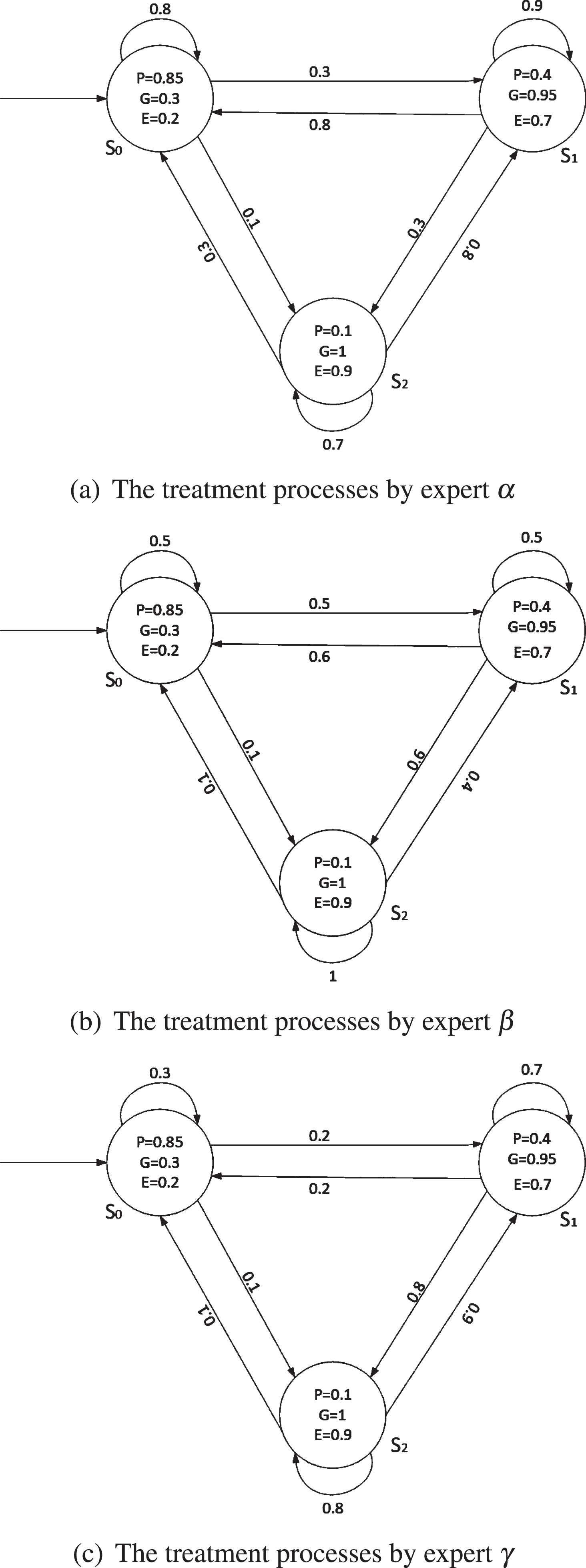
This study extends the existing approach of the generalized possibilistic model checking to solve quantitative reachability problems. Li et al. [17, 18, 21, 22] propose possibility model checking and generalized possibility model checking in combination with measure theory, providing a solution to the existing problems of fuzzy model checking. In [17], the reachability problem based on the possibility measure is given, and the reachability problem is studied by using a possibilistic Kripke structure as a model. In the existing generalized possibilistic model checking, the generalized possibilistic Kripke structure is the formal model of the representation system. However, in real life, a generalized possibilistic Kripke structure cannot describe nondeterministic and concurrent fuzzy systems. For example, suppose three experts want to formulate treatment schemes for a new bacterial infection. Because different experts have different understandings of the disease, each expert has a different scheme. We use a generalized possibilistic Kripke structure K = (S, P, I, AP, L) to model the patient’s treatment process respectively. It describes three treatment processes given by three experts(α, β and γ) in Fig. 1(a), (b), (c). However, the generalized possibilistic Kripke structure can only represent the treatment process of a scheme, cannot describe the joint consultation of three experts. To solve this problem, we propose a generalized possibilistic decision process to describe nondeterministic and concurrent fuzzy systems.
Fig. 1
The treatment processes by three experts.
In this paper, we mainly study the maximum possibility problem and the minimum possibility problem of eventual reachability, always reachability, constrained reachability, repeated reachability and persistent reachability under a generalized possibilistic decision process. First, we propose a generalized possibilistic decision process as the model of fuzzy systems, and deduce the possibilities of sets of paths of the generalized possibilistic decision process relying on defining of schedulers. Then, the fuzzy matrices calculation methods of reachability under a generalized possibilistic decision process are given, and the results show that the compositional operations of the fuzzy matrix is polynomial time, which is better than the exponential level of existing algorithms. Finally, we propose a model checking approach to convert the verification of safety property into the analysis of reachabilities.
The rest of this paper is organized as follows. Section 2 gives some preliminary knowledge. In Section 3, we define generalized possibilistic decision processes. In Section 4, we present the fuzzy matrix calculation methods of eventual reachability, always reachability, constrained reachability, repeated reachability and persistent reachability. In Section 5, we use good prefixes to analyze the possibilistic regular safety property. Section 6 is the conclusion. The proofs of some theorems of this paper can be found in the Appendix.
2Preliminaries
To model and verify fuzzy systems, we provide some necessary knowledge including the fuzzy set, fuzzy set operation, fuzzy matrix operation, closure and others.
Definition 1. [23, 26, 28] Let X be a universal set. A fuzzy set A of X is an function which associates each element in X a value in the interval [0, 1], i.e., A : X ⟶ [0, 1]. For x ∈ X, A (x) is the membership of x in the fuzzy set A.
We use
Definition 2. [26, 28] Let
(A ∪ B) (x) = A (x) ∨B (x) = max {A (x) , B (x)},
(A ∩ B) (x) = A (x) ∧ B (x) = min {A (x) , B (x)},
Ac (x) =1 - A (x).
Definition 3. [26, 28] Let R and S be two fuzzy matrices with m rows and n columns, i.e., R = (rij) m×n, S = (sij) m×n. We introduce some set operators.
R = S if and only if rij = sij for all i, j.
R ⊆ S if and only if rij ≤ sij for all i, j.
R ∪ S = (rij∨sij) m×n.
R ∩ S = (rij ∧ sij) m×n.
Rc = (1 - rij) m×n.
Definition 4. [26, 28] Let R be a fuzzy matrix with m rows and n columns, and S be a fuzzy matrix with n rows and l columns, i.e., R = (rij) m×n and S = (sij) n×l. The composition operation of R and S is R ∘ S = (tij) m×l, where
(R ∘ S) ∘ T = R ∘ (S ∘ T);
(R ∪ S) ∘ T = (R ∘ T) ∪ (S ∘ T).
Let X be a universal set. For the fuzzy matrix R = (R (s, t)) s,t∈X, we use R+ to denote its transitive closure. When X is finite, X has ∣X∣ elements, then R+ = R ∪ R2 ∪ . . . ∪ R∣X∣, where Rk+1 = Rk ∘ R for any positive integer number k. The Kleene closure R* = R0 ∪ R+, for each 1≤ s, t ≤ ∣ S ∣,
Definition 5. [21] Let X be a nonempty set,and Ω be a set composed of some subsets of X elements. We call Ω a σ- algebra, which is closed to countable and take complement set operations. The possibility measure on σ- algebra Ω is a mapping POS : Ω → [0, 1], which satisfies the following conditions:
(1) POS (∅) =0;
(2) POS (X) =1;
(3) If Ei ∈ Ω, i ∈ I, then POS (⋃ i∈IEi) = ⋁ i∈IPOS (Ei)
If only conditions(1) and (3), then POS is called a generalized possibility measure. If POS is a generalized possibility measure on the power set 2X,for any A ⊆ X, there is POS (A) = ⋁ a∈APOS ({ a }).
Definition 6. [18] A Generalized possibilistic Kripke structure(GPKS) is a tuple K = (S, P, I, AP, L), where
(1) S is a countable, nonempty states set;
(2) P : S × S → [0, 1] is the possibility transition distribution, for any states s, there is a state t, such that P (s, t) >0;
(3) I : S → [0, 1] is the initial distribution of possibility and there exists a state s, such that I (s) >0;
(4) AP is a set of atomic propositions;
(5) L : S × AP → [0, 1] is a label function, L (s, a) represents the true value of atomic proposition a in state s.
For a GPKS K, its path is defined as an infinite sequence of states π = s0s1s2 ⋯ ∈ s
ω, for any i so that P (si, si+1) > 0. Let Paths (s) and Pathsfin (s) represent the set of all infinite and finite paths starting from the state s in K. Paths (K) represents the set of all infinite paths in K, Pathsfin (K) represents the set of all finite paths in K, such as
3Generalized Possibilistic Decision Processes
In this section, first, we give the notion of the generalized possibilistic decision process. Then, the definition of the scheduler is proposed to solve the nondeterministic the generalized possibilistic decision process. Finally, we solve the generalized possibility measure problems.
Nondeterminism is absent in GPKS. The generalized possibilistic decision process can be viewed as a variant of GPKS that permits both possibility and nondeterministic choices.
Definition 7. A Generalized possibilistic decision process(GPDP) is a tuple M = (S, Act, P, I, AP, L), where
(1) S is a countable, nonempty set of states;
(2) Act is a set of actions;
(3) P : S × Act × S ⟶ [0, 1] is a function, called possibilistic transition distribution function. For all states s ∈ S and actions α ∈ Act, there exits a state t ∈ S such that P (s, α, t) >0;
(4) I : S ⟶ [0, 1] is a function, there exits states s such that I (s) >0;
(5) AP is a set of atomic propositions;
(6) L : S × AP ⟶ [0, 1] is a possibilistic labeling function, which can be viewed as function mapping a state s to the fuzzy set of atomic proposition, L (s, a) denotes the possibility or truth value of atomic proposition a which is hold in state s.
Furthermore, if the set S, Act and AP are finite sets, then M is a finite GPDP. In this paper, we always assume that GPDPs are finite. A GPDP has a unique initial distribution I. For all states s, t ∈ S and actions α ∈ Act, P (s, α, t) denotes the possibility from state s under action α to state t. An action α is enabled in state s if and only if P (s, α, t) >0. Let Act (s) denote the set of enabled actions in state s. For any states s ∈ S, it is required that Act (s)≠ ∅. Each state t for which P (s, α, t) >0 is called an α-successor of s. The set of direct α-successors of s is defined as:
Post (s, α) = {t ∈ S ∣ P (s, α, t) >0}.
The set of α-predecessors of s is defined by:
Pref (t) = {(s, α) ∈ S × Act (s) ∣ P (s, α, t) >0}.
We also use the P (s, α, T) to denote the possibility from the state s under the action α to the set T of states, that is,
Paths in GPDP M are defined as infinite alternating sequences π = s0
α0s1
α1s2 ⋯ ∈ (S × Act)
ω such that P (si, αi, si+1) >0 for all i ∈ I. Paths (s) denotes the set of all infinite paths in M that start in state s. Similarly, Pathsfin (s) denotes the set of all finite path fragment
Example 1. Let us consider the joint consult of three experts in Fig. 1(a),(b),(c). GPDP in Fig. 2, where states are represented by ovals and transitions by labeled edges, and state names are depicted outside the ovals, and labeling functions of the states are depicted inside the ovals.
Fig. 2
Treatment process by three experts’ consultation.
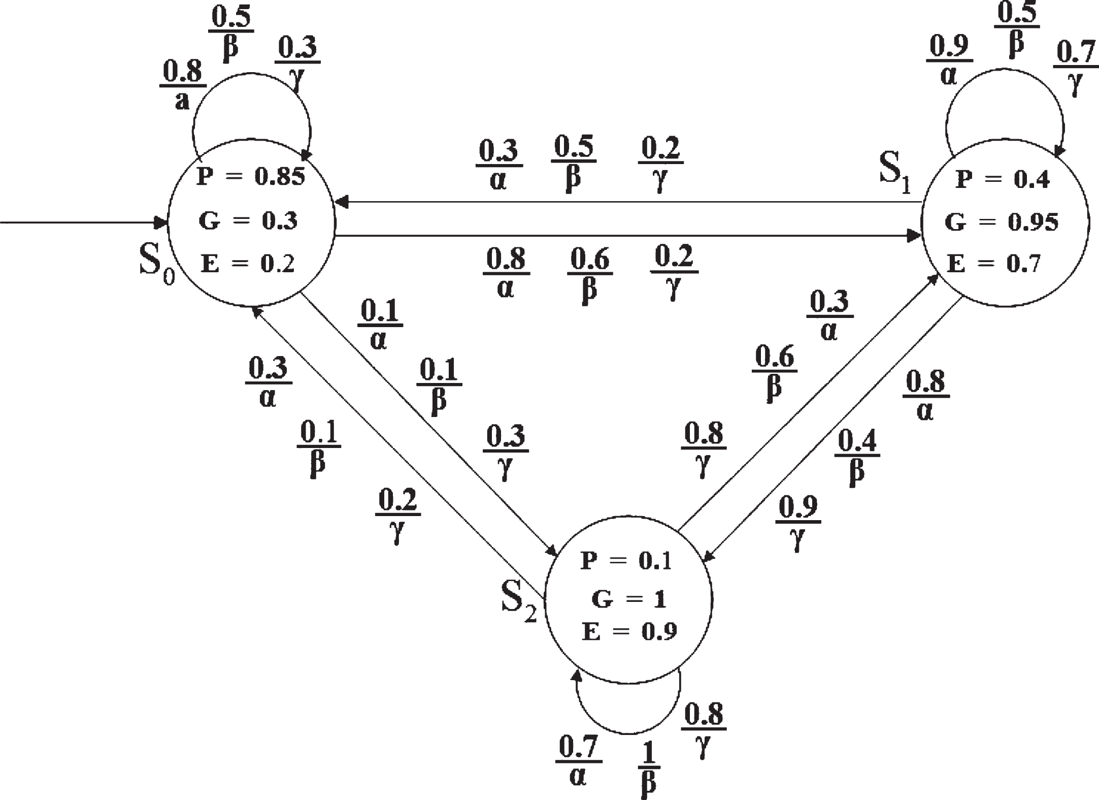
S = {s0, s1, s2}, Act = {α, β, γ}, AP = {P, G, E}. P indicates that the patient is in “bad” health, G indicates that the patient is in “normal” health, E indicates that the patient is in “good” health.
For state s0, the labeling functions are L (s0, P) =0.85, L (s0, G) =0.3, L (s0, E) =0.2. L (s0, P) =0.85 indicates that the degree of “bad” health in state s0 is 0.85. L (s0, G) =0.3 indicates that the degree of “normal” health in state s0 is 0.3. L (s0, E) =0.2 indicates that the degree of “good” health in state s0 is 0.2.
Act (s0) = {α, β, γ}, α, β, γ indicate three different treatment indicates. P (s0, α, s1) =0.8 indicates that the possibility of the patient’s health condition changing from state s0 to state s1 is 0.8 after the expert treats the patient with the α scheme. P (s0, β, s1) =0.6 indicates that the possibility of the patient’s health condition changing from state s0 to state s1 is 0.6 after the expert treats the patient with the β scheme. P (s0, γ, s1) =0.2 indicates that the possibility of the patient’s health condition changing from state s0 to state s1 is 0.2 after the expert treats the patient with the γ scheme.
Post (s0, α) = {s1, s2},Post (s0, α) indicates all α successor states of state s0.
Pref (s0) = {(s0, α) , (s0, β) , (s0, γ) , (s1, α) , (s1, β) ,
(s1, γ) , (s2, α) , (s2, β) , (s2, γ)}, Pref (s0) indicates all predecessor states of state s0.
For the GPKS K, 2Paths (K) is the algebra that is generated by
Definition 8. Let M = (S, Act, P, I, AP, L) be a GPDP, a scheduler for M is a function Adv : S → 2Act so that Adv (s) ⊆ Act (s) for all s ∈ S.
Let PathAdv (s) and
Given a GPDP M = (S, Act, P, I, AP, L), α ∈ Act, possibility distribution function P : S × α × S ⟶ [0, 1] can be represented by a fuzzy matrix. For convenience, the fuzzy matrix is written as P
α, so that P
α = (P (s, α, t)) s,t∈S, called the fuzzy transition matrix of M corresponding to scheduler α. Using fuzzy matrix
Using fuzzy matrix
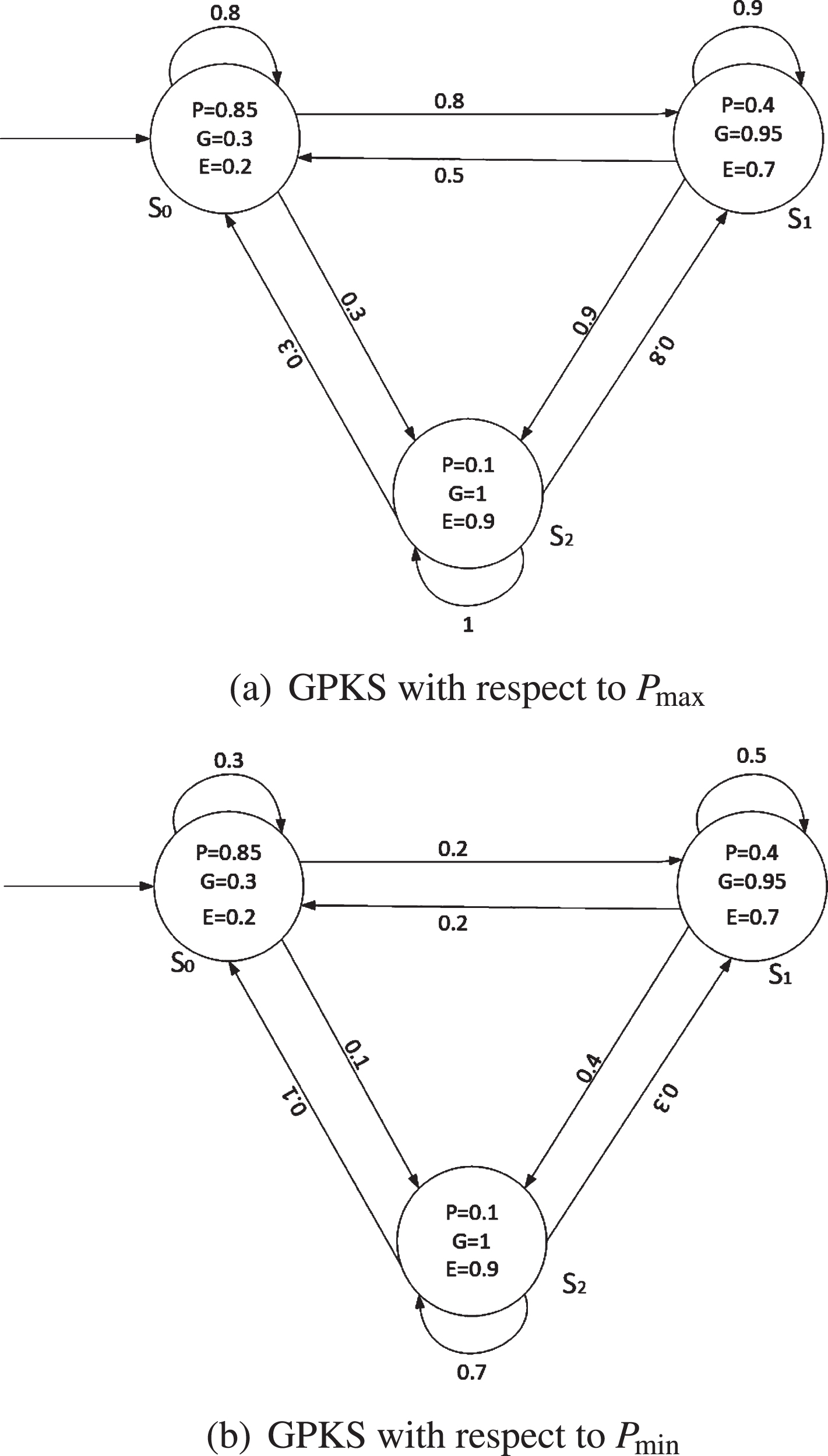
The GPKS Kmax = (S, Pmax, I, AP, L) and GPKS Kmin = (S, Pmin, I, AP, L) can be constructed from matrix Pmax and matrix Pmin respectively.
Example 2. As shown in the Example 1, the order of s0→s1→s2 is used to give the fuzzy matrices Pmax, Pmin.
Figure 3(a) shows the result of GPKS with respect to Pmax, Fig. 3(b) shows the result of GPKS with respect to Pmin.
Fig. 3
GPKS with respect to Pmax and Pmin.
Although GPDP can induce the GPKS under the consideration of some schedulers, reasoning about quantitative reachabilities requires a formalization of the possiblities for sets of paths. This formalization is based on possibility measure theory, in particular possibility spaces and generalized possibility measure theory.
Definition 9. Given a GPDP M = (S, Act, P, I, AP, L), let
(1)
The cylinder set spanned by the finite adv-paths
Definition 10. Let M = (S, Act, P, I, AP, L) be a finite GPDP, the function GPo : PathsAdv (M) → [0, 1] is defined:
(2)
Let M = (S, Act, P, I, AP, L) be a GPDP, s ∈ S, αi ∈ Act, i ≥ 0, rAdv : S → [0, 1] is defined as following, which denotes the maximal possibility measure of all Adv-paths from state s in M:
(3)
The role of the function rAdv is to help us to calculate the possibility of Adv-paths in M. The Theorem 1 gives a fuzzy matrix calculation for rAdv.
Theorem 1. Let M = (S, Act, P, I, AP, L) be a finite GPDP, for any s ∈ S, then we have
(4)
In particular, PAdv is normal iff rAdv (s) =1 for any states s.
Proof. See the Appendix. ■
In the matrix notation, we have
(5)
The computational complexity of rAdv (s) mainly depends on the time of computational possibilistic transition closure. In [30], they gave an optimal algorithm to calculate DAdv, then we get the time complexity is O (n2 log n), where n =∣ S ∣.
Example 3. According to the GPDP in Example 1, for any s ∈ S,rmax and rmin corresponding to the maximal scheduler and the minimal scheduler are given,
rmax (s0) = 0.8 indicates that under the maximal possibilistic scheduler. That is, the maximal possibility of all paths from state s0 is 0.8. rmin (s0) = 0.3 indicates that under the minimal possibilistic scheduler. That is, the maximal possibility of all paths from state s0 is 0.3.
Based on Theorem 1, we can get Theorem 2, which can convert the calculation of generalized possibility measure of infinite path into the calculation of possibility of finite path.
Theorem 2. Let M = (S, Act, P, I, AP, L) be a finite GPDP, then the generalized possibility measure of cylinder set
Proof. See the Appendix. ■
Example 4. According to the GPDP of Example 1, under the maximal possibilistic measure and the minimal possibilistic measure, the generalized possibility measure of cylinder set of the corresponding finite paths
GPomax (Cyl (s0 α0s1) ) = I (s0) ∧ P (s0, α0, s1) ∧ rmax (s1) =0.8
GPomin (Cyl (s0 α0s1)) = I (s0) ∧ P (s0, α0, s1) ∧ rmin (s1) =0.5 .
4Reachability possibility
A typical task for the quantitative analysis of GPDPs is to compute the minimum or the maximum possibility for some reachabilities under consideration of the min or the max scheduler. This corresponds to the worst-case or best-case analysis possibility of GPDPs. Let M = (S, Act, P, I, AP, L) be a finite GPDP and B be a fuzzy set of target states. The fuzzy set B may represent a set of certain bad states that shall be visited with the minimum possibility, or dually, a set of good states that shall be visited with the maximum possibility. Some special reachabilities, such as eventual reachability, always reachability, constrained reachability, repeated reachability and persistent reachability are considered in this section.
4.1Eventual reachability possibility
The event of eventual reachability is denoted ⋄B. We use the B : S ⟶ [0, 1] to represent the fuzzy set of states. For the given GPDP M, π = s0 α0s1 … ∈ PathsAdv (M), ∣∣ ⋄ B (π) ∣∣ = ⋁ i≥0B (si). In the following, the quantitative analysis of eventual reachability is reduced to the computational range for all strategies of the minimum possibility or the maximum possibility of reaching a certain fuzzy set B of states.
Theorem 3. Let M = (S, Act, P, I, AP, L) be GPDP, max corresponds to the maximum possibility scheduler and min corresponds to the minimum possibility scheduler, then we have,
(6)
(7)
Proof. See the Appendix. ■
Example 5. Based on Example 1, consider the generalized possibility of eventual reachability event ⋄B. Given the fuzzy state set B = (L (s, E)) s∈S, only the reachability of the event is considered at this point, and the label function in GPDP is defined as L (s) = s.
Then the maximum possibility and minimum possibility of the event ײ7B are respectively:
∥GPo (◊ ≤7B) ∥ max (s0) =0.8, ∥GPo (◊ ≤7B) ∥ min (s0) =0.2, describes the maximum possibility of the patient’s final state of health with the maximum possibility of “good” being 0.8 and the minimum possibility of “good” being 0.2 after 7 days treatment from state s0.
4.2Always reachability possibility
The event of always reachability is denoted B. We use the B : S ⟶ [0, 1] to represent the fuzzy set of states. For the given GPDPs M, π = s0 α0s1 … ∈ PathsAdv (M), B (π) = ⋀ i≥0B (si). Under the maximum possibility scheduler and the minimum possibility scheduler, the methods of computing GPomax (s ⊨ B) and GPomin (s ⊨ B) are given.
Theorem 4. Let M = (S, Act, P, I, AP, L) be GPDPs, max corresponds to the maximum possibility scheduler and min corresponds to the minimum possibility scheduler, then we have
(8)
(9)
Example 6. Based on Example 1, considering the generalized possibility of always reachability event ≤7B, given the fuzzy state set B = (L (s, E)) s∈S, the maximum possibility and the minimum possibility of all states in M satisfied event ≤7B are respectively:
fz1 = fz2, Therefore
Calculated by the same method
∥GPo ( E) ∥ max (s0) =0.2, ∥GPo ( E) ∥ min (s0) =0.2, it shows that from the state s0, it is unlikely that the patient’s health always reach a “good” state after 7 days treatment.
4.3Constrained reachability possibility
Given the GPDP M, and the fuzzy set of states B, C : S ⟶ [0, 1], consider the event of reaching B via a finite path fragment which ends in a fuzzy state s ∈ B, and visits only states in set of fuzzy states C prior to reaching fuzzy states s. This event is denoted by C ⊔ B. For n ≥ 0, the event C ⊔ ≤nB has the same meaning as C ⊔ B, and it is required to reach B(via fuzzy state C) within n steps. Formally, C ⊔ ≤nB is the union of the basic cylinders spanned by path fragments s0 α0s1 α1 … sm so that m ≤ n with possibility C (si) for all 0 ≤ i ≤ m with possibility B (sk).
Theorem 5. Let M = (S, Act, P, I, AP, L) be a GPDP, max corresponds to the maximum possibility scheduler and min corresponds to the minimum possibility scheduler, then we have
(10)
(11)
Proof. See the Appendix. ■
Example 7. Next, let’s continue to consider the generalized possibility of constrained reachability event C ⊔ ≤7B. Given the fuzzy state set C = (L (s, P)) s∈S, B = (L (s, E)) s∈S, the maximum possibility and the minimum possibility of all states in M satisfying event C ⊔ ≤7B are respectively:
∥GPo (C ⊔ ≤7B) ∥ max (s0) =0.7, ∥GPo (C ⊔ ≤7B) ∥ min (s0) =0.2, which means that the patient’s health state is “bad” at state s0. The expert adopts three treatment schemes after 7 days of treatment, the maximum possibility that a patient’s health states turn to a “good” state is 0.7 and the minimum possibility is 0.2.
4.4Repeated reachability possibility
Let B : S ⟶ [0, 1] be a set of fuzzy states in GPDPs. For the event of repeated reachability, we use the ⋄ B to represent it. The set of all paths that visit B infinitely is often measurable. Let π = s0
α0s1
α1 … ∈ PathsAdv (s0),
Theorem 6. Let M = (S, Act, P, I, AP, L) be a GPDP, B : S ⟶ [0, 1] is a fuzzy set of states, max corresponds to the maximum possibility scheduler and min corresponds to the minimum possibility scheduler. Then we have,
(12)
(13)
Proof. See the Appendix. ■
Example 8. Next, let’s continue to consider the generalized possibility of the repeated reachability event ⋄ B. Given the fuzzy state set B = (L (s, P)) s∈S, the maximum possibility and the minimum possibility of all states in M satisfying event ⋄ B are respectively:
When the state is s0, ∥GPo ( ⋄ B) ∥ max (s0) =0.8, ∥GPo ( ⋄ B) ∥ min (s0) =0.3, indicates that the patients in this state are more likely to relapse. When the state is s2, ∥GPo ( ⋄ B) ∥ max (s2) =0.1, ∥GPo ( ⋄ B) ∥ min (s0) =0.1, indicates that once the patient’s disease in this state is cured, and it basically will not recur.
4.5Persistent reachability possibility
Let us consider persistent reachability properties events of the form ⋄ B. Let π = s0
α0s1
α1 … ∈ PathsAdv (s0) and B : S ⟶ [0, 1] be a fuzzy set of states in GPDPs. Thus,
Theorem 7. Let M = (S, Act, P, I, AP, L) be a GPDP, B : S ⟶ [0, 1] is the fuzzy set of states, max corresponds to the maximum possibility scheduler and min corresponds to the minimum possibility scheduler.
(14)
(15)
Proof. See the Appendix. ■
Example 9. Next, continue to consider the generalized possibility of persistent reachability event ⋄ B. Given the fuzzy state set B = (L (s, E)) s∈S, the maximum possibility and the minimum possibility of all states in M satisfied event ⋄ B are respectively,
The possibility that the patient’s health continue to be “good” after the expert adopts the combination of three schemes. When the state is s0, ∥GPo (⋄ B) ∥ max (s0) =0.2, ∥GPo (⋄ B) ∥ min (s0) =0.2, which indicates that the patient is in a bad state of health and is already in a state of illness. For state s2, ∥GPo (⋄ B) ∥ max (s2) =0.9, ∥GPo (⋄ B) ∥ min (s2) =0.7, which indicates that the patient’s state health has been in a “good” state.
5Reachability in the safety properties
The analysis of safety properties and the techniques for checking safety properties are closely related to reachability. Safety properties are often characterized as “nothing bad should happen”. In classic model checking, safety properties are defined as linear property which does not include a bad prefix, and analyses the eventual reachability and repeated reachability. Since it is difficult to define the notion of a bad prefix in fuzzy logic or possibility logic, Li [21] uses the good prefixes to define the fuzzy safety property, and computes the always reachability possibility and persistent reachability possibility. In the following section, we use the good prefixes to analyze the possibilistic of regular safety property.
For a GPDP M = (S, Act, P, I, AP, L), we assume the alphabet Σ = lAP for some finite subset l ⊆ [0, 1] in the following.
Definition 11.c4:def1 For the safety property Psafe, we define a possibilistic language Gref (Psafe) : Σ* ⟶ [0, 1] as Gpref (Psafe) (θ) = ⋁ {Psafe (θσ) ∣ σ ∈ Σ ω}. For all θ ∈ Σ*, Gpref (Psafe) is called the good prefixes of Psafe.
Psafe is called possibilistic regular safety property if Psafe (σ) = ⋀ {Gpref (Psafe) (θ) ∣ θ ∈ Gpref (σ) }, for all σ ∈ Σ ω, Pref (σ) = {θ ∈ Σ* ∣ σ = θσ′, σ′ ∈ Σ ω} is called the set of prefixes of σ.
We call Psafe a generalized possibilistic regular safety property if Psafe is a generalized possibilistic safety property and Gpref (Psafe) is a fuzzy regular language over Σ.
Definition 12. [22] A fuzzy finite automata is a five tuple A = (Q, Σ, δ, Q0, F), where
(1) Q is a finite nonempty set of states;
(2) Σ a finite nonempty set of input symbols;
(3) δ : Q × Σ × Q ⟶ [0, 1] is a fuzzy transition function. For any p, q ∈ Q, a ∈ Σ, δ (p, a, q) denotes the possibility of state p reaching state Q under the action of input letter a;
(4) Q0 : Q ⟶ [0, 1] represent the fuzzy initial state of fuzzy automata A,for q ∈ Q,Q0 (q) denotes q is the possibility of the initial state;
(5) F : Q ⟶ [0, 1] represent the fuzzy acceptance state of fuzzy automata A,F (q) denotes q is the possibility of the acceptance state;
For a GPDP M = (S, Act, P, I, AP, L) and a fuzzy finite automata A = (Q, Σ, δ, Q0, F), the product of M and A is defined as follows.
Definition 13. Let M = (S, P, Act, I, AP, L) be a GPDP, A = (Q, Σ, δ, Q0, F) be a fuzzy finite automata, M ⊗ A = (S × Q, P′, Act′, I′, AP′, L′), where P′ (< s, q > , α, < s′, q′ >) = P (s, α, s′) ∧ δ (q, L (s′) , q′); Act′ (< s, q >) = Act (s); I′ (< s, q >) = I (s) ∧ ⋁ q0∈QQ0 (q0) ∧ δ (q0, L (s) , q); for all <s, q > ∈ S × Q, AP′ = S × Q; L′ (< s, q >) = < s, q >.
For each path π = s0 α0s1 α1s2 α2 … ∈ PathsAdv (M) in M, TraceAdv (π) = L (s0) L (s1) L (s2)…, the fuzzy automata A has a unique run q0q1q2… and in M ⊗ A there exists π+ =< s0, q1 > α0 < s1, q2 > α1 … corresponding to them.Similarly, the path in M ⊗ A with state <s0, δ (q0, L (s))> also corresponds to the path in M and the run in A.
Theorem 8.Let M = (S, Act, P, I, AP, L) be a GPDP, Psafe is the generalized possibilistic regular safety property accepted by a deterministic fuzzy finite automata A = (Q, Σ, δ, Q0, F), and Adv is the set of all strategies begin state s. We have:
(16)
Proof. See the Appendix. ■
Let GPoAdv ( B) = GPoAdv (s ⊨ B) s∈S, then
GPoAdv ( B) can be solved by the maximum fixed point, where the maximum fixed point of the operator is fB (Z) = B ∧ PAdv ∘ DZ ∘ rAdv. For the scheduler Adv taking the maximum possibility scheduler max and the minimum possibility scheduler min, the maximum possibility and the minimum possibility that the state s satisfies the generalized possibilistic regular safety property P are respectively:
(17)
(18)
Example 10. We use Example 1 as a sample. To discuss the generalized possibility measure of generalized possibilistic regular safety property in the alphabet Σ = lAP, in which
Fig. 4
Finite automata A corresponding to Gref (Psafe).
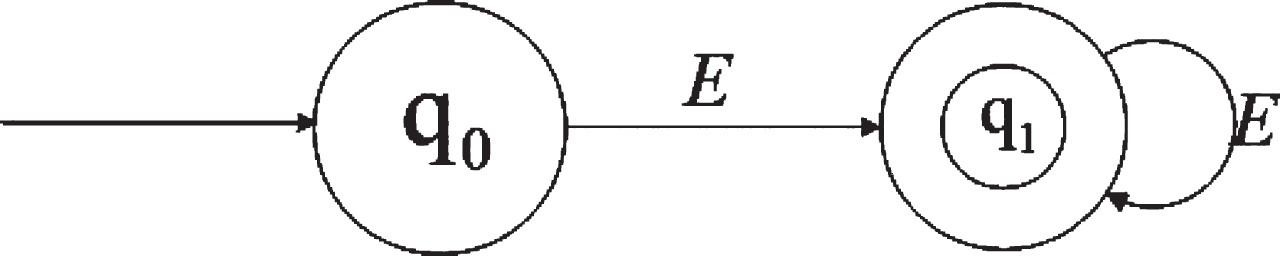
Given a GPDP M and generalized possibilistic regular safety property Psafe = {A0, A1, … ∈ Σ ω ∣ ∀ i ≥ 0, Ai (E) >0}, Adv is the scheduler defined in M. The solution processes of GPomax (s0 ⊨ Psafe) and GPomin (s0 ⊨ Psafe) corresponding to Adv is the maximum scheduler and the minimum scheduler are given.
The product M ⊗ A of a GPDP M and Psafe good prefix Gref (Psafe) corresponding to a finite automata A is shown in Fig. 5. According to formulas 17 and 18, there B = S × {q1} = {1, 1, 1} is
Fig. 5
Product GPDPs M ⊗ A.
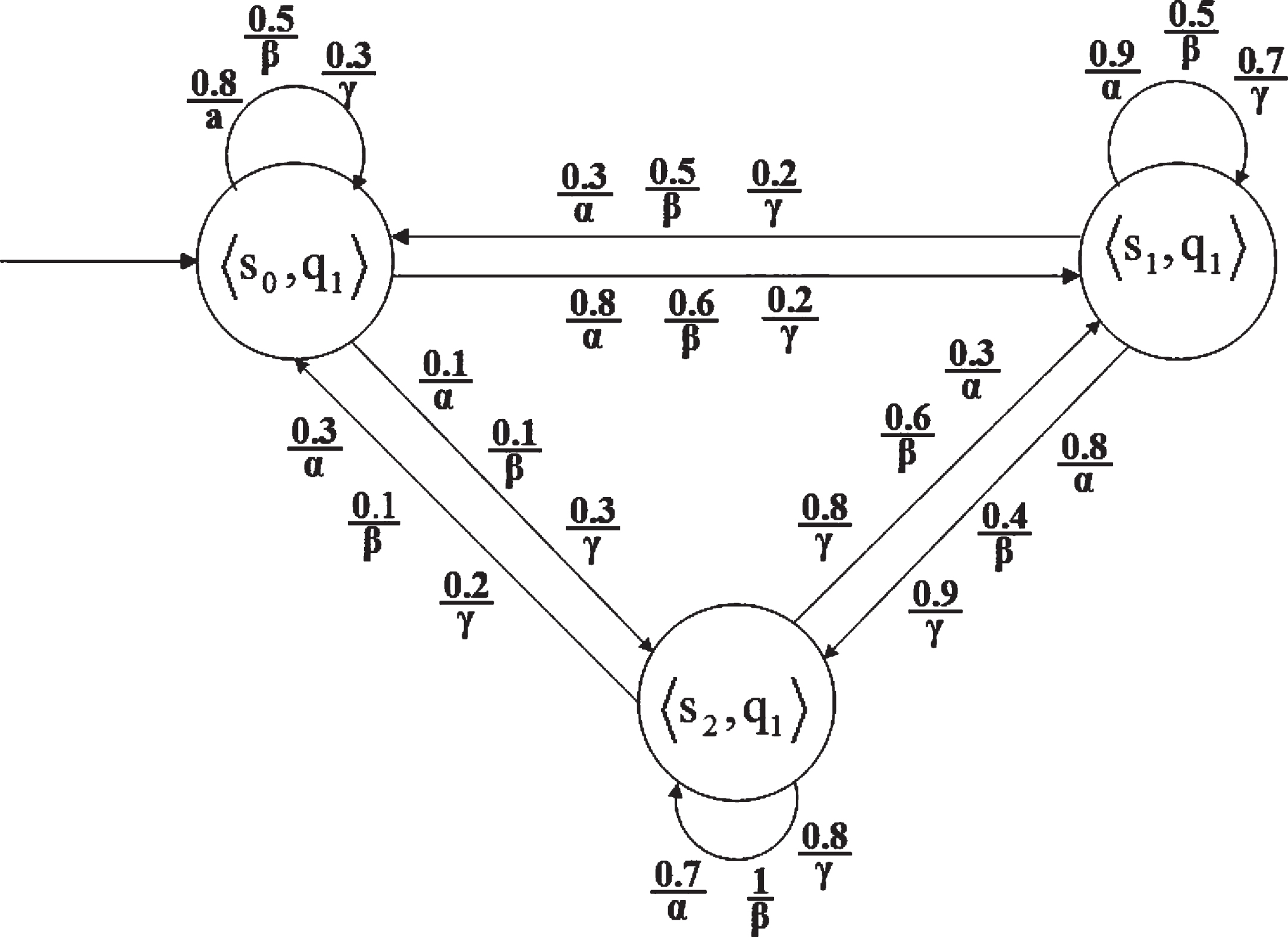
fz1 = fz2, Therefore
Calculated by the same method
GPomax (s0 ⊨ Psafe) =0.8,GPomin (s0 ⊨ Psafe) =0.3 are obtained, which shows that the maximum possibility and minimum possibility of generalized possibilistic regular safety property Psafe in GPDPs M are 0.8 and 0.3.
6Conclusion
In this paper, firstly, we propose GPDPs as the models of nondeterministic and concurrent fuzzy systems. Then, we give fuzzy matrices calculation methods of the maximal possibilities and the minimal possibilities of reachabilities. Finally, we propose a model checking approach to convert the verification of safety property into the analysis of reachabilities. We have given the method of optimization algorithm for reachability. In the future, we will investigate the optimization algorithm for reachability to solve the verification of other properties, such as liveness and fairness in fuzzy systems.
Acknowledgments
The work is partially supported by National Natural Science Foundation of China(Grant No. 61962001), Graduate Innovation Project of North Minzu University(Grant No. YCX22184 and No. YCX22196).
Appendix
Proof. [Proof of Theorem 1]
Since S and Act is finite, given the scheduler Adv, the possibility transition matrix PAdv is also finite. Obviously, the fuzzy meet operator ∧ does not generate new element,so the set
In this case, PAdv (s, α0, s1)∧ PAdv (s1, α1, s2) ∧ ⋯
= PAdv (s, α0, s1) ∧ ⋯ ∧ PAdv (si-1, αi-1, t) ∧ (PAdv (t, αi, si+1)
∧⋯ PAdv (sj-1, αj, t)) ∧ ⋯
≤PAdv (s, α0, s1) ∧ ⋯ ∧ PAdv (si-1, αi-1, t) ∧ (PAdv (t, αi, si+1)
∧ ⋯ ∧ PAdv (sj-1, αj, t))
Hence,
Conversely, for any t ∈ S and schedulers Adv, by the definition of
Let πAdv = s0
α0s1
α1 ⋯ si-1
αi-1tαi (si+1 ⋯ sj αjt)
ω,then
Hence,
Therefore,
Proof. [Proof of Theorem 2]
From
Therefore, GPo (Cyl (s0 α0 ⋯ αn-1sn) )
= ⋁ {GPo (πAdv) ∣ s0 α0 ⋯ αn-1sn ∈ Pref (πAdv)}
Proof. [Proof of Theorem 3]
GPomax (s ⊨ ⋄ B)
= ⋁ π∈Pathsmax(s) (GPomax (π) ∧ ∥ ⋄ B ∥ (π) )
where Pmaxis the maximum possibility transition matrix under the max scheduler, Kleene closure of Pmax is
GPomin (s ⊨ ⋄ B)
= ⋁ π∈Pathsmin(s) (GPomin (π) ∧ ∥ ⋄ B ∥ (π) )
where Pmin is the minimum possibility transition matrix under the min scheduler.
Proof. [Proof of Theorem 5]
GPomax (s ⊨ C ⊔ ≤nB) = ⋁ π∈Pathsmax(s) (GPomax (π) ∧ ∥ C ⊔ ≤nB ∥ (π) )
= ⋁ (⋁ α0∈Act(s0)P (s0, α0, s1) ∧ ⋁ α1∈Act(s1)P (s1, α1, s2)
GPomin (s ⊨ C ⊔ ≤nB)
= ⋁ π∈Pathsmin(s) (GPomin (π) ∧ ∥ C ⊔ ≤nB ∥ (π) )
Proof. [Proof of Theorem 6]
GPoAdv (s ⊨ ⋄ B) = ⋁ π∈PathsAdv(s) (GPo (π) ∧ ∥ ⋄ B ∥ (π) ). Let π = s0 α0s1 α1 … ∈ PathsAdv (s0), inf (π) denotes the set of states that occur infinitely many times on the path π, then ∥ ⋄ B ∥ (π) ≤ ⋁ t∈inf(π)B (t). Furthermore, for any t ∈ inf (π), π ⊨ ⋄ t, we can get GPoAdv (π) ≤ GPoAdv ({π ∈ Pathsfin (s) ∣ π ⊨ ⋄ t} ) , thus GPoAdv (π) ∧ ∥ ⋄ B ∥ (π) ≤ ⋁ t∈inf(π) > (B (t) ∧ GPoAdv (s ⊨ ⋄ t) ) ≤ ⋁ t∈S (B (t) ∧ GPoAdv (s ⊨ ⋄ t) ) . Therefore, GPoAdv (s ⊨ ⋄ B) ≤ ⋁ t∈S (B (t) ∧ GPoAdv (s ⊨ ⋄ t) ) .
Conversely, for any state t ∈ S, and any path π ∈ PathsAdv (s) that satisfies the event ⋄ t,we have B (s) ≤ ∥ ⋄ B ∥ (π). It follows that ⋁t∈S (B (t) ∧ GPoAdv (s ⊨ ⋄ t) ) ≤ ⋁ t∈S (B (t) ∧ GPoAdv (s ⊨ ⋄ t) ), therefore, ⋁t∈S (B (t) ∧ GPoAdv (s ⊨ ⋄ t) ) ≤ GPoAdv (s ⊨ ⋄ B).
In conclusion, GPoAdv (s⊨ ⋄ B) = ⋁ t∈SB (t) ∧
GPoAdv (s ⊨ ⋄ t) .
We can get the method to calculate GPoAdv (s ⊨ ⋄ t) from these results, that is
When the Adv is the maximum possibility scheduler and the minimum possibility scheduler, we can get Theorem 6.
Proof. [Proof of Theorem 7]
GPomax (s ⊨ ⋄ B)
= ⋁ π∈Pathsmax(s) (GPomax (π) ∧ ∥ ⋄ B ∥ (π) )
∧B (si+1) ∧ ⋁ αi+1∈ActP (si+1, αi+1, si+2) ∧ B (si+2) ∧ … )
B (si+2) ∧ … )
∧ (Dmax ∘ Pmax) (si, si+1) ∧ (Dmax ∘ Pmax) (si+1, si+2)
∧ … )
∧rDB∘Pmax (si) )
Pmax (si-1si) ∧ rDB∘Pmax (si) )
GPomin (s ⊨ ⋄ B)
= ⋁ π∈Pathsmin(s) (GPomin (π) ∧ ∥ ⋄ B ∥ (π) )
Proof. [Proof of Theorem 8]
= ⋁ π∈PathsAdv(s) (GPoAdv (π) ∧ Psafe (TraceAdv (π)) )
= ⋁ (GPoAdv (π) ∧ ⋀ j≥0 {L (A) (θ) ∣ θ ∈ Pref (TraceAdv (π)) } )
= ⋁ (GPoAdv (π) ∧ ⋀ j≥0 {F (qj) ∣ qjδ* (q0, L (s) L (s1) … L (sj)) } ) ⋁ (GPoAdv (π) ∧ ⋀ i≥0F (qi) ) .
For π = sα0s1 α1 … ∈ PathsAdv (s), we define the run sequence q0q1q2… of the deterministic fuzzy finite automata by qi+1 = δ (qi, L (si)). Vice versa, for the same run sequence q0q1q2… of the deterministic fuzzy finite automata, we have
= ⋁ π+∈PathsAdv(<s,qs>) (GPoAdv (π+) ∧ ⋀ i≥0B (π+ [i]) )
= ⋁ π∈PathsAdv(s) (GPoAdv (π) ∧ ⋀ i≥0F (qi) ) ,
References
[1] | Mahmood I. A Verification Framework for ComponentBased Modeling and Simulation Putting the pieces together[J], arXiv preprint arXiv:2301.03088, 2023. |
[2] | Pan H. , Li Y. , Cao Y. et al. Model checking fuzzy computation tree logic[J]. Fuzzy sets and Systems 262: ((2015) ), 60–77. |
[3] | Laroussinie F. et al. Principles of Model Checking[J]. The Computer Journal 53: (5) ((2010) ), 615–616. |
[4] | Hansen H.A. , Schneider G. and Steffen M. , Reachability analysis of complex planar hybrid systems[J]. Science of Computer Programming 78: (12) ((2013) ), 2511–2536. |
[5] | Herbert S.L. , Bansal S. , Ghosh S. et al. Reachability-based safety guarantees using efficient initializations[C], 2019 IEEE 58th Conference on Decision and Control (CDC), IEEE, 2019, 4810–4816. |
[6] | Wang J. , Deng Y. and Xu G. , Reachability analysis of real-time systems using time Petri nets. IEEE Trans Syst Man Cybern B Cybern 30: (5) ((2000) ), 725–736. doi: 10.1109/3477.875448. PMID: 18252405 |
[7] | Bouyer P. , Markey N. , Randour M. et al. Reachability in networks of register protocols under stochastic schedulers[J], arXiv preprint arXiv:1602.05928, 2016. |
[8] | Xie D. , Xiong W. , Bu L. et al. Deriving unbounded reachability proof of linear hybrid automata during bounded checking procedure[J]. IEEE Transactions on Computers 66: (3) ((2016) ), 416–430. |
[9] | Ganguli S. , Iyer C.V.K. , Pandey V. Reachability Embeddings: Scalable Self-Supervised Representation Learning from MobilityTrajectories for Multimodal Geospatial Computer Vision[C], 2022 23rd IEEE International Conference on Mobile Data Management (MDM), IEEE, 2022, 44–53. |
[10] | Song Y.H. , Shahid S. and Chung E.S. , Differences in multi-model ensembles of CMIP5 and CMIP6 projections for future droughts in South Korea[J]. International Journal of Climatology 42: (5) ((2022) ), 2688–2716. |
[11] | Li Y. , Droste M. and Lei L. , Model checking of linear-time properties in multi-valued systems[J]. Information Sciences 377: ((2017) ), 51–74. |
[12] | Ma Z. , Li Z. , Li W. et al. Model Checking Fuzzy Computation Tree Logic Based on Fuzzy Decision Processes with Cost[J]. Entropy 24: (9) ((2022) ), 1183. |
[13] | Lee N. , Kim Y. , Kim M. et al. Directed Model Checking for Fast Abstract Reachability Analysis[J]. IEEE Access 9: ((2021) ), 158738–158750. |
[14] | Wang Y. , Yuan Y. , Zhang W. et al. Reachability-Driven Influence Maximization in Time-dependent Road-social Networks[C], 2022 IEEE 38th International Conference on Data Engineering (ICDE), IEEE, 2022, 367–379. |
[15] | Wu D. and Koutsoukos X. , Reachability analysis of uncertain systems using bounded-parameter Markov decision processes[J]. Artificial Intelligence 172: (8-9) ((2008) ), 945–954. |
[16] | Wu D. and Koutsoukos X. , Reachability analysis of uncertain systems using bounded-parameter Markov decision processes[J]. Artificial Intelligence 172: (8-9) ((2008) ), 945–954. |
[17] | Li Y. and Li L. , Model checking of linear-time properties based on possibility measure[J]. IEEE Transactions on Fuzzy Systems 21: (5) ((2012) ), 842–854. |
[18] | Li Y. and Wei J. , Possibilistic fuzzy linear temporal logic and itsmodel checking[J]. IEEE Transactions on Fuzzy Systems 29: (7) ((2020) ), 1899–1913. |
[19] | Jiang J. , Zhang P. and Ma Z. , The μ-calculus model-checkingalgorithm for generalized possibilistic decision process[J]. Applied Sciences 10: (7) ((2020) ), 2594. |
[20] | Am A. , Mp B. , Sr C. et al. Model-checking graded computation-tree logic with finite path semantics[J]. Theoretical Computer Science 806: ((2020) ), 577–586. |
[21] | Li Y. , Quantitative model checking of linear-time properties based on generalized possibility measures[J]. Fuzzy sets and Systems 320: ((2017) ), 17–39. |
[22] | Li Y. and Ma Z. , Quantitative computation tree logic model checking based on generalized possibility measures[J]. IEEE Transactions on Fuzzy Systems 23: (6) ((2015) ), 2034–2047. |
[23] | Ying S. and Ying M. , Reachability analysis of quantum Markov decision processes[J], . Information and Computation 263: ((2018) ), 31–51. |
[24] | Huang S. and Cleaveland R. , A tableau construction for finite linear-time temporal logic[J]. Journal of Logical and Algebraic Methods in Programming 125: ((2022) ), 100743. |
[25] | Quatmann T. , Junges S. , Katoen J.P. Markov automata with multiple objectives[C], International Conference on Computer Aided Verification, Springer, Cham, 2017, 140–159. |
[26] | Shojafar M. , Javanmardi S. , Abolfazli S. et al. FUGE: A joint meta-heuristic approach to cloud job scheduling algorithm using fuzzy theory and a genetic method[J]. Cluster Computing 18: (2) ((2015) ), 829–844. |
[27] | Wei X. and Li Y. , Fuzzy alternating automata over distributive lattices[J]. Information Sciences 425: ((2018) ), 34–47. |
[28] | Madhumangal Pal Fuzzy Matrices with Fuzzy Rows and Columns, 1 Jan. 2016, 561–573. |
[29] | Wang Q. , Li R. , Ying M. Equivalence Checking of Sequential Quantum Circuits[J], IEEE Transactions on Computer-Aided Design of Integrated Circuits and Systems, 2021. doi: 10.1109/TCAD.2021.3117506. |
[30] | Garmendia L. , Salvador , Gonzĺćlez del R. , Campo , Lĺöpez et al. An algorithm to compute the transitive closure, a transitive approximation and a transitive opening of a fuzzy proximity[J]. Mathware and Soft Computing 16: (2) ((2009) ), 175–191. |
[31] | Hartmanns A. , Junges S. , Katoen J.P. et al. Multi-cost bounded reachability in MDP[C], International Conference on Tools and Algorithms for the Construction and Analysis of Systems, Springer, Cham, 2018, 320–339. |
[32] | Chondrogiannis T. , Nascimento M.A. , Bouros P. Relative reachability analysis as a tool for urban mobility planning: Position paper[C], Proceedings of the 12th ACM SIGSPATIAL International Workshop on Computational Transportation Science, 2019, 1–4. |


