Hyperplane-based time-aware knowledge graph embedding for temporal knowledge graph completion

He, Peng; Zhou, Gang; Liu, Hongbo; Xia, Yi; Wang, Ling

doi:10.3233/JIFS-211950

Hyperplane-based time-aware knowledge graph embedding for temporal knowledge graph completion

Article type: Research Article

Authors: He, Peng^{a; b} | Zhou, Gang^{a; *} | Liu, Hongbo^a | Xia, Yi^a | Wang, Ling^a

Affiliations: [a] Information Engineering University, China | [b] Zhengzhou University of Technology, China

Correspondence: [*] Corresponding author. Gang Zhou, Information Engineering University, China. Tel.: +86 371 8162 2551; Fax: +86 371 8162 2551; E-mail: [email protected].

Keywords: Temporal knowledge graph, knowledge graph completion, knowledge graph embedding

DOI: 10.3233/JIFS-211950

Journal: Journal of Intelligent & Fuzzy Systems, vol. 42, no. 6, pp. 5457-5469, 2022

Published: 28 April 2022

Get PDF

Abstract

Knowledge Graph (KG) embedding approaches have been proved effective to infer new facts for a KG based on the existing ones–a problem known as KG completion. However, most of them have focused on static KGs, in fact, relational facts in KGs often show temporal dynamics, e.g., the fact (US, has president, Barack Obama, [2009–2017]) is only valid from 2009 to 2017. Therefore, utilizing available time information to develop temporal KG embedding models is an increasingly important problem. In this paper, we propose a new hyperplane-based time-aware KG embedding model for temporal KG completion. By employing the method of time-specific hyperplanes, our model could explicitly incorporate time information in the entity-relation space to predict missing elements in the KG more effectively, especially temporal scopes for facts with missing time information. Moreover, in order to model and infer four important relation patterns including symmetry, antisymmetry, inversion and composition, we map facts happened at the same time into a polar coordinate system. During training procedure, a time-enhanced negative sampling strategy is proposed to get more effective negative samples. Experimental results on datasets extracted from real-world temporal KGs show that our model significantly outperforms existing state-of-the-art approaches for the KG completion task.

1Introduction

Knowledge Graphs (KGs) collect and store human knowledge as large multi-relational directed graphs where nodes represent entities, and typed edges represent relationships between entities. Examples of real-world KGs include Freebase [1], YAGO [2] and WordNet [3]. Each fact in a KG can be represented as a form of triple such as (US, has president, Barack Obama) where ‘US’ and ‘Barack Obama’ are called head and tail entities respectively and ‘has president’ is a relation connecting them. In the past few years, we have witnessed the great achievement of KGs in many areas, such as natural language processing [4], question answering [5], recommendation systems [6], and information retrieval [7]. Although commonly used real-world KGs contain billions of triples, they still suffer from the incompleteness problem that a lot of valid triples are missing. Therefore, there have been various studies on predicting missing relations or entities based on the existing ones which is an import problem known as KG completion or link prediction. As one of the most effective approaches, KG embedding has state-of-the-art results for KG completion on many benchmarks.

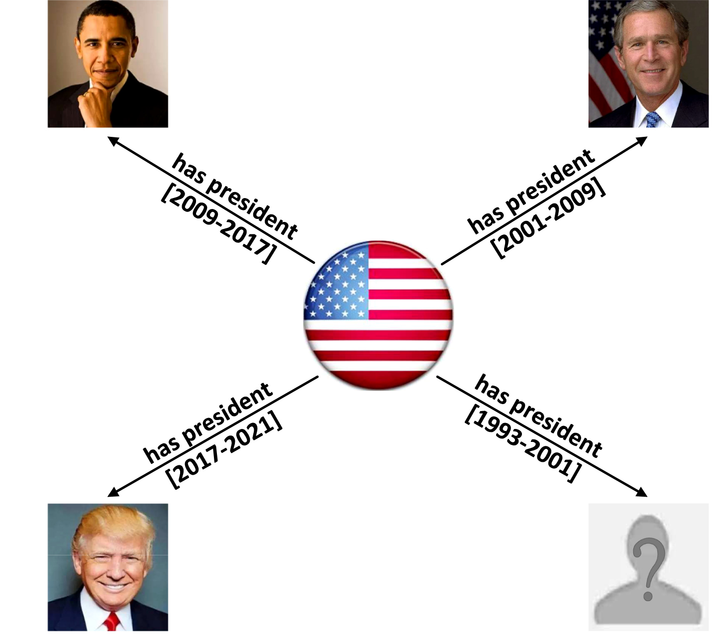
KG embedding is also called KG representation learning, which aims to represent entities and relations in low-dimensional continuous vector spaces, so as to simplify manipulation while preserving the inherent structure and semantics of the KG. Traditionally, a KG is considered to be a static snapshot of multi-relational data. And the traditional KG embedding approaches (see [8–10] for a summary) have been mostly designed for this kind of static KGs, which ignore the availability and importance of temporal aspect while learning vectorial representations (also called embeddings) of entities and relations. However, in several well-known temporal KGs, such as Integrated Crisis Early Warning System (ICEWS) [11], Global Database of Events, Language, and Tone (GDELT) [12], YAGO3 [13] and Wikidata [14], facts are typically associated with timestamps and might only hold for a point in time or a certain time interval. For example, Fig. 1 shows a subgraph of such temporal KG, in which the fact (US, has president, Barack Obama, [2009–2017]) is only valid from 2009 to 2017. As a result, developing embedding learning solely on the basis of static facts as in static KG embedding approaches will confuse entities with similar semantics when conduct KG completion. For example, they may confuse entities such as ‘Barack Obama’ and ‘Bill Clinton’ when predicting the missing tail entity of (US, has president, ?, [1993–2001]). To conquer this problem, several temporal KG embedding approaches have been designed to answer this kind of query accurately. That is, the ranking of the query (US, has president, ?, timestamp) is expected to vary with the different timestamps.

Fig. 1

A sample temporal knowledge subgraph extracted from the Wikidata.

Most of the existing temporal KG embedding models incorporate time information during representation learning explicitly or implicitly by extending static approaches. And the vast majority of them can only deal with time information in the form of points in time but have difficulty in handling time information in the form of time intervals as in Fig. 1. In fact, time information in the form of time intervals is universal and has illustrated a common challenge posed by its time continuity. On the other hand, the success of a KG embedding model is heavily dependent on its ability to model and infer connectivity patterns of the relations, such as symmetry (e.g., marriage), antisymmetry (e.g., filiation), inversion (e.g., hypernym and hyponym) and composition (e.g., my mother’s husband is my father) [15]. However, few existing temporal KG embedding models could model and infer all the above relation patterns. A more detailed description can be referred to in section 3.

To address the above issues, we propose a novel Hyperplane-based Time-aware Knowledge graph Embedding model named HTKE for temporal KG completion. By dividing time information from the input KG into multiple time-specific hyperplanes representing distinct time in points or time periods, and projecting facts to time-specific hyperplanes which they belong to according to their timestamps, our model could incorporate explicitly and utilize time information directly. Meanwhile, our model can deal with timestamps not only in the form of points in time but also in the form of time intervals, and predict temporal scopes for facts with missing timestamps such as (US, has president, Barack Obama, ?). In addition, the proposed model is capable of modeling and inferring all the above four important relation patterns including symmetry, antisymmetry, inversion and composition through mapping facts happened at the same time into a polar coordinate system. We illustrate that the HTKE is scalable to large KGs as it remains linear in both time and space complexity.

We further propose a time-enhanced negative sampling strategy to get more effective negative samples for optimization, which generates negative samples by corrupting both entities and timestamps of known facts. To evaluate the performance and merits of our model, we conduct extensive experiments on temporal datasets extracted from ICEWS and YAGO3 for KG completion and temporal scope prediction tasks. Experimental results show that our method significantly and consistently outperforms the state-of-the-art models.

The organization of the paper is as follows. Section 2 presents some formal background and reviews the related work. In Section 3, we first describe the details of our model. Then, we show that how our model can infer four relation patterns. Finally, we discuss the scalability of our model and the process of optimization. Section 4 reports experimental results and in Section 5, we conclude the paper and discuss future work.

2Background and related work

Notation: Throughout this paper, we present scalars with lower-case letters, vectors with bold lower-case letters and tensors with bold upper-case letters. Let z∈ℝd be a real vector of length d, z∈ℂd be a complex vector of length d. [z] _i represents the i-th entry of a vector z, and ||z||_l represents its l norm.

Temporal Knowledge Graph (Completion): Let E be a finite set of entities, R be a finite set of relation types, and T be a finite set of timestamps. W⊂E×R×E×T represent the collection of all temporal facts which have the form of a quadruple (head, relation, tail, timestamp), or (h, r, t, τ) and (h, r, t, [τ_s, τ_e]) for short, where h,t∈E represents the head and tail entities respectively, r∈R represents relations connecting two entities, τ,[τs,τe]∈T represents timestamps of quadruples. Specifically, the former expresses facts occurred at a specific point in time τ, and the latter expresses facts occurred at an (open) time interval with start time τ_s and end time τ_e. A temporal KG G is a subset of W (i.e., G⊂W ). Temporal KG completion is a problem of inferring W from G . As shown in Fig. 1, the aim of temporal KG completion (i.e. link prediction) is to predict the missing element of the quadruple (US, has president, ?, [1993–2001]) on the basis of all known quadruples including (US, has president, Barack Obama, [2009–2017]), (US, has president, Donald Trump, [2017–2021]), etc.

Relation Patterns: According to the existing literatures [15–19], four types of relation patterns are very important and widely spread in real-world KGs: symmetry, antisymmetry, inversion and composition. We give their formal definition here:

Definition 1. A relation r is symmetric if

(h,r,t,τ)∈W⇔(t,r,h,τ)∈W

Definition 2. A relation r is antisymmetric if

(h,r,t,τ)∈W⇔(t,r,h,τ)∈Wc

where Wc is the complement of W .

Definition 3. A relation r₁ is inverse to relation r₂ if

(h,r1,t,τ)∈W⇔(t,r2,h,τ)∈W

Definition 4. A relation r₁ is composed of relation r₂ and relation r₃ if

(h,r2,e,τ)∈W∧(e,r3,t,τ)∈W⇒(h,r1,t,τ)∈W

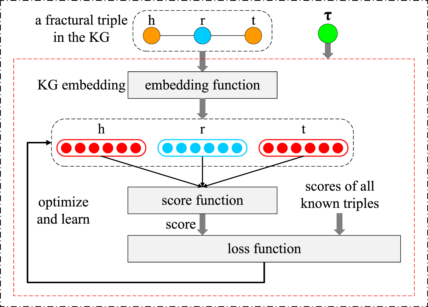
(Temporal) KG Embedding: KG embedding is also called KG representation learning. As Fig. 2 shows, a KG embedding model defines three things: 1- the embedding function for mapping entities and relations to vector spaces, 2- a score function which takes embeddings for h, r and t as input and generates a score as the factuality for the given triple (h, r, t), 3- a suitable loss function to optimize and learn the values of embeddings using all known triples in the input KG. The values of the embeddings are learned using all known facts in the KG. Temporal KG embedding is to incorporate time information available such as timestamps τ during representation learning to improve the performance of embedding.

Fig. 2

A simple illustration of KG embedding.

During the past decade, a variety of KG embedding models have been widely explored for the KG completion task. In the following, we will introduce two lines of them that are closely related to our work. One is the static KG embedding method which learns vectorial embeddings only on the basis of static triples and ignoring available time information; the other is the temporal KG embedding method, which leverages time information associated with known facts during representation learning to improve the performance of embedding. The embedding representations and score functions of several typical static and temporal models are listed in Table 1, where 〈 · , · 〉 is the sum of Hadamard (element-wise) product of vectors [20], t¯ is the complex conjugate of t [16], r^-1 is the inverse relation embedding of relation r, e→,e←∈ℝd and e ∈ {h, t} is the vectorial representations of entities located in the head and tail position respectively [21], ∘ is the element-wise product of vectors [15]. For each τ∈T , τ∈ℝd and τ∈ℂd are vectorial embeddings of timestamps [22, 23]. x_⊥ = x - τ^Txτ where x ∈ {h, r, t} denotes the temporal projection of embeddings [24]. LSTM (·) is an LSTM neural network and r_seq denotes a temporal relation embedding [25]. T∈ℝd3 is the time-specific core tensor [26]. e→t,e←t∈ℝd and e ∈ {h, t} are temporal entity embeddings [27]. For further details on these methods, please refer to recent surveys [28–30].

Table 1

Embedding representations and scoring functions of state-of-the-art static and temporal models

	Model	Embedding representations	Scoring function
Static	TransE (2013)	h,t∈ℝd , r∈ℝd	- ∥ h + r - t ∥ _1/2
	DistMult (2014)	h,t∈ℝd , r∈ℝd	〈h, r, t〉
	ComplEx (2016)	h,t∈ℂd , r∈ℂd	Re (〈h,r,t¯〉)
	SimplE (2018)	h→,h←,t→,t←∈ℝd , r,r-1∈ℝd	12(〈h→,r,t←〉+〈t→,r-1,h←〉)
	RotatE (2019)	h,t∈ℂd , r∈ℂd	-\|\|h ∘ r - t\|\|₁
Temporal	TTransE (2018)	h,t∈ℝd , r∈ℝd,τ∈ℝd	- ∥ h + r + τ - t ∥ _1/2
	HyTE (2018)	h,t∈ℝd , r∈ℝd	-\|\|h_⊥ + r_⊥ - t_⊥\|\|_1/2
	TA-TransE (2018)	h,t∈ℝd,rseq∈ℝd	- ∥ h + LSTM (r_seq) - t ∥ ₂
	TA-DistMult (2018)	h,t∈ℝd,rseq∈ℝd	〈h, LSTM (r_seq) , t〉
	ConT (2019)	h,t∈ℝd , r∈ℝd,T∈ℝd3	〈T, h ∘ r ∘ t〉
	DE-SimplE (2020)	h→τ,h←τ,t→τ,t←τ∈ℝd , r,r-1∈ℝd	12(〈h→τ,r,t←τ〉+〈t→τ,r-1,h←τ〉)
	TComplEx (2020)	h,t∈ℂd , r∈ℂd,τ∈ℂd	Re (〈h,r,t¯,τ〉)

2.1Static KG embedding models

Most of the existing KG embedding approaches are static and can be roughly divided into two categories, translational distance-based models [15, 31–33] and tensor factorization models [16, 20, 21, 34]. Translational distance-based models use the distance between two entities as a metric to measure the plausibility of facts, usually after a translation or rotation carried out by relations. TransE [31] is a typical translational distanced-based model. It maps facts into a real vector space and interprets the relation as a translation from the head to the tail. The score function is defined as the Euclidean distance between the translated head embedding and tail embedding. TransE can implicitly model the antisymmetry, inversion and composition relation patterns, but has difficulty in modeling the symmetry relation pattern which is common in real-world KGs. To overcome this drawback, many variations of TransE have been proposed, such as RotatE [15] and HAKE [32]. Compared with TransE, RotatE maps each triple into a complex vector space instead of a real vector space, and considers the relation as a rotation from the head embedding to the tail embedding in the complex vector space. In this way, RotatE could model and infer all four important types of relation patterns mentioned above. Moreover, HAKE is a slight extension of RotatE. By taking advantage of both the modulus and phrase part of the complex vector, HAKE is able to model not only all of the above relation patterns but also semantic hierarchies between entities.

Apart from translation distance-based models, tensor factorization models are also competitive on many benchmarks, including DistMult [20], ComplEx [16] and SimplE [21]. DistMult defines the same embedding function as in TransE, but the score function is the sum of Hadamard (element-wise) product of embedding vectors. Intuitively, DistMult is a simplified version of the tensor factorization model, which learns a symmetric tensor in the head and tail modes to keep the parameter sharing. As a result, it can only model symmetric relations and cannot infer antisymmetric relations. ComplEx enhances DistMult by mapping elements into a complex space, where head and tail embeddings share the parameters of values but are complex conjugate of each other. SimplE is another tensor factorization approach based on Canonical Polyadic (CP) decomposition [35], which employs inverse relations to associate two embeddings of the same entity locating at different positions. Compared with ComplEx, SimplE avoids computational redundancy and reduces time consumption. Besides, Lacroix et al. [34] also proposed a similar CP decomposition-based model to improve the performance.

Although static models have achieved great success, their representing and modeling capabilities are still limited due to the single static triples. Therefore, all kinds of extensions of static KG embedding models have been developed by infusing rich additional information into the process of representation learning, including time information, entity types, relation paths, etc. Especially time information, which demonstrates the specific time when an event happened or a fact was valid, can effectively avoid entity confusion and improve the performance of KG embedding.

2.2Temporal KG embedding models

Many temporal KG embedding models have been explored and most of them can be seen as extensions of static models. Such as, TTransE [22], HyTE [24] and TA-TransE [25] are extended from TransE, TA-DistMult [25] is the temporal extension of DistMult. Similar to their static versions TransE and DistMult, these temporal KG embedding models have issues with inferring symmetric relations or antisymmetric relations. Recently, TComplEx and TNTComplEx [23] follow CP decomposition to extend ComplEx by adding a new temporal factor vector. Therefore, same as ComplEx, TComplEx and TNTComplEx also involve the problem of redundant computations. DE-SimplE [27] learns entity embeddings that evolve over time by introducing a diachronic entity (DE) embedding function. As an extension of SimplE, DE-SimplE has the capability of encoding domain knowledge by parameter sharing and is the first full expressive temporal KG embedding model. ConT [26] can be seen as an extension of Tucker [36] which replaces the core tensor in Tucker decomposition [37] with a time-specific tensor. Both DE-SimplE and ConT do not take into account facts with time intervals shaped like [2015, 2018] and are hard to predict time scopes for facts missing time information. Moreover, because of the large number of parameters per timestamp, ConT faces a high time complexity and rapid overfits during training. Inspired by RotatE, ChronoR interprets the relation and time together as a rotation from the head entity to the tail entity, and represents entities, relations and timestamps as matrices in real vector space. While the operation of the matrices brings high time and space costs. In contrast, HERCULES [38], which is a time-aware extension of the static model ATTH [39] learns embeddings in hyperbolic spaces rather than Euclidean space. But similar to DE-SimplE and ConT, HERCULES cannot model timestamps with the form of time intervals. On the other hand, recent T-GAP [40] incorporates neural network and additional relation path information to the process of temporal KG embedding, which aims to fully exploit the local neighborhood and facilitate multi-hop reasoning. However, both neural network and path traversal are time-consuming.

In contrast, our proposed model HTKE has merits to conquer these issues. That is, our model could deal with time information not only in the form of points in time but also in the form of time intervals, and predict temporal scopes for facts with missing time information. Furthermore, our model is capable of modeling and inferring all four important relation patterns including symmetry, antisymmetry, inversion and composition with linear time and space consuming.

All of the above temporal KG embedding models, including our method can be classified as the interpolation setting. Under this setting, models attempt to infer missing links at past timestamps. While most recently, several work [41–45] attempt to predict facts in the future, which is called the extrapolation setting. Under the extrapolation setting, models can better support the open-world assumption that missing facts is not necessarily false and may potentially happen in the future, which is also the direction of our future work.

3The proposed HTKE

In this section, we introduce our proposed model Hyperplane-based Time-aware Knowledge graph Embedding model (HTKE). Generally speaking, our model contains two components, one is the time-specific hyperplane, and the other is a polar coordinate system.

3.1Time-specific hyperplane

As mentioned above, temporal KGs provide time information of facts. In order to incorporate these time information directly during KG embedding algorithm, for a KG with time information in the form of points in time, we dismantle it into n disjoint time point subgraphs G = G_τ₁ ∪ G_τ₂ ∪ … ∪ G_{τ_n}, where ∀i≠ j, G_{τ_i} ∩ G_{τ_j} = ∅ and τ_i (i ∈ 1, 2, ⋯ , n) is one of the time points. For a KG with time information in the form of time intervals, we dismantle it into n disjoint time period subgraphs G = G_τ₁ ∪ G_τ₂ ∪ … ∪ G_{τ_n}, where ∀i≠ j, G_{τ_i} ∩ G_{τ_j} = ∅ and τ_i (i ∈ 1, 2, ⋯ , n) is one of the time periods with minimum time min(τ_i), maximum time max(τ_i). Each quadruple belongs to one or more time subgraphs according to its timestamp. Such as, if the timestamp is a specific point in time with the form of τ, then it only belong to one time point subgraph G_{τ_i} when τ = τ_i. While if the timestamp of a quadruple is a time interval with the form of [τ_s, τ_e], then it may belong to one time period subgraph G_{τ_i} or more time period subgraphs G_{τ_i} … G_{τ_j} when min(τ_i) ≤ τ_s ≤ τ_e ≤ max(τ_i) or min(τ_i) ≤ τ_s ≤ max(τ_i) ≤ … ≤ min(τ_j) ≤ τ_e ≤ max(τ_j).

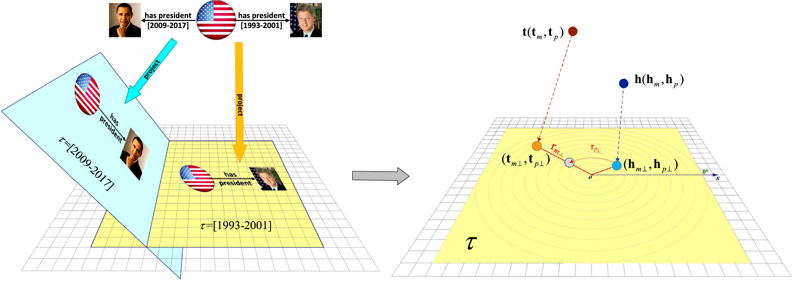
Then, each time subgraph is associated with a time-specific hyperplane represented by a normal vector τ, where τ∈ℝd and ||τ_i||₂ = 1. Thus, we can get n different hyperplanes represented by normal vectors τ₁, τ₂, …, τ_n. That is to say, we can segregate the space into n different time zones with the help of these time-specific hyperplanes.

Subsequently, we project each fact to time-specific hyperplanes which it belongs to. Such as Fig. 3 shows, we project two facts with time information (US, has president, Barack Obama, [2009-2017]) and (US, has president, Bill Clinton, [1993-2001]) onto different time-specific hyperplanes denoted by normal vectors τ = [2009 - 2017] and τ = [1993 - 2001]. In this way, facts happened at different times can be distinguished. Therefore, its easy to conclude the correct answer ‘Bill Clinton’ when answering the the query (US, has president, ?, [1993-2001]) mentioned in section 1.

Fig. 3

Simple illustration of our proposed HTKE.

3.2Polar coordinate system

In order to model and infer four common and important relation patterns introduced in section 2, we further map facts projected on the same time-specific hyperplane into a polar coordinate system. Specifically, we first map each entity e to two parts–the modulus part em∈ℝd and the phase part e_p ∈ [0, 2π) ^d, where the modulus part corresponds to the radial coordinate and the phase part corresponds to the angular coordinate. Thus the projections of entities on the time-specific hyperplane τ can be represented as projected modulus parts:

(1)

em⊥=em-(τ⊤emτ),

and the projected phase part:

(2)

ep⊥=ep-(τ⊤epτ).

On this hyperplane, we consider every dimension of projected entity representation, i.e., ([e_m⊥] _i, [e_p⊥] _i) as a 2D point in the polar coordinate system. Inspired by static models RotatE and HAKE, we interpret each relation as a rotation from the projected head angular coordinate [h_p⊥] _i to the projected tail angular coordinate [t_p⊥] _i plus a scaling transformation form the projected head radial coordinate [h_m⊥] _i to the projected tail radial coordinate [t_m⊥] _i. Therefore, the relation r should also be mapped to two parts rm∈ℝ+d and r_p ∈ [0, 2π) ^d where r_m represents the extent of scalability, r_p represents the rotation angle. These two parts are also projected onto the corresponding time-specific hyperplane. Given a quadruple (h, r, t, τ), we adopt the basic idea of translation distance-based models, using the distance between the head entity transformed by the relation and the tail entity in the polar coordinate system to measure the factuality of this quadruple. Alternatively, for a positive quadruple, we expect that the head entity embedding rotated and scaled by the relation embedding is as close to the tail entity embedding as possible and otherwise, they are expected to be far away. As a result,the score function is defined as

(3)

φ(h,r,t,τ)=-‖hm⊥∘rm⊥-tm⊥‖2-λ‖sin((hp⊥+rp⊥-tp⊥)/2)‖1

where the first part -||h_m⊥ ∘ r_m⊥ - t_m⊥||₂ represents the distance between the head entity after scaling by the relation and the tail entity in the radial coordinate, and the second prat -|| sin((h_p⊥ + r_p⊥ - t_p⊥)/2) ||₁ represents the distance between the head entity after rotation by the relation and the tail entity in the angular coordinate. The smaller the distance, the higher the score. The sin function is used in the second part because the angular coordinates have periodic characteristics and λ∈ℝ is a parameter that is learned by the model. Figure 3 gives an illustration of the proposed model.

Table 2

Time complexity and number of parameters for each model considered, d is the dimension of the embedding vector space

Model	Time complexity	Number of parameters
TTransE	O (d)	d(\|E\|+\|R\|+\|T\|)
HyTE	O (d)	d(\|E\|+\|R\|+\|T\|)
TA-TransE	O (d)	d(\|E\|+\|R\|+\|T\|)
TA-DistMult	O (d)	d(\|E\|+\|R\|+\|T\|)
ConT	O (d³)	d(\|E\|+\|R\|)+d3\|T\|
DE-SimplE	O (d)	d(2(3γ+(1-γ))\|E\|+2\|R\|)
TComplEx	O (d)	d(2\|E\|+4\|R\|+2\|T\|)
HTKE	O (d)	d(2\|E\|+2\|R\|+\|T\|)

3.3Model and inference relation patterns

Our method can model and infer all four important relation patterns including symmetry, antisymmetry, inversion and composition. On time-specific hyperplane τ, similar to RotatE and HAKE, a relation r is symmetric(antisymmetric) if and only if each element of its projected rotation angle [r_p⊥] _i satisfies [r_p⊥] _i = kπ ([r_p⊥] _i ≠ kπ) , k = 0, 1, 2; two relations r₁ and r₂ are inverse if and only if each element of their projected rotation angles is opposite to each other: [r_1p⊥] _i = - [r_2p⊥] _i; a relation r₁ is a combination of other two relations r₂ and r₃ if and only if each element of their projected rotation angle satisfy [r_1p⊥] _i = [r_2p⊥] _i + [r_3p⊥] _i. Figure 3 shows how HTKE models these relation patterns with only 1-dimensional embedding.

Lemma 1. HTKE can infer the symmetry/antisymmetry relation pattern in time-specific hyperplanes.

Proof. If (h, r, t, τ) and (t, r, h, τ) hold in their corresponding time-specific hyperplane τ, we have

(4)

tp⊥=(hp⊥+rp⊥)mod2π∧hp⊥=(tp⊥+rp⊥)mod2π⇒∀i,[rp⊥]i=kπ,k=0,1,2

Otherwise, if (h, r, t, τ) and ¬ (t, r, h, τ) hold, we have

(5)

tp⊥=(hp⊥+rp⊥)mod2π∧hp⊥≠(tp⊥+rp⊥)mod2π⇒∃i,[rp⊥]i≠kπ,k=0,1,2

Lemma 2. HTKE can infer the inversion relation pattern in time-specific hyperplanes.

Proof. If (h, r₁, t, τ) and (t, r₂, h, τ) hold in their corresponding time-specific hyperplane τ, we have

(6)

tp⊥=(hp⊥+r1p⊥)mod2π∧hp⊥=(tp⊥+r2p⊥)mod2π⇒∀i,[r1p⊥]i=-[r2p⊥]i

Lemma 3. HTKE can infer the composition relation pattern in time-specific hyperplanes.

Proof. If (h, r₁, t, τ), (h, r₂, e, τ) and (e, r₃, t, τ) hold in their corresponding time-specific hyperplane τ, we have

(7)

tp⊥=(hp⊥+r1p⊥)mod2π∧ep⊥=(hp⊥+r2p⊥)mod2π∧tp⊥=(ep⊥+r3p⊥)⇒∀i,[r1p⊥]i=[r2p⊥]i+[r3p⊥]i

3.4Time complexity and parameter growth

As described in [46], to scale to the size of current KGs and keep up with their growth, a KG embedding model must have a linear time and space complexity. Models with many parameters usually overfit and present poor scalability. We calculate and analyze the time complexity and the number of parameters for several state-of-the-art temporal KG embedding approaches and our model according to embedding functions and score functions of models, which are listed in Table 2, where d is the dimension of the embedding vector space. Contrary to DE-SimplE, other models do not learn temporal embeddings that scale with the number of entities (as frequencies and biases), but rather embeddings that scale with the number of timestamps. Although our model has more parameters than HyTE, but experiments demonstrate that our model performs better than HyTE because of the ability to model the symmetry relation pattern. All of the temporal models except for ConT have the linear time complexity O (d). The large number of parameters per timestamp (a three-order tensor) makes ConT perform poorly and train extremely slowly. As an extension of ComplEx, TComplEx also involves redundant computations.

Table 3

Statistics on ICEWS14, ICEWS05-15, and YAGO11k

Dataset	\|E\|	\|R\|	\|T\|	\|train\|	\|validation\|	\|test\|
ICEWS14	7,128	230	365	72,826	8,941	8,963
ICEWS05-15	10,488	251	4017	386,962	46,275	46,092
YAGO11k	10,623	10	198	164,000	2000	2000

3.5Optimization

To train the model, we use the negative sampling loss function with self-adversarial training [15]:

(8)

L=∑x∈G+∑y∈G-,

where γ is a fixed margin, σ is the sigmoid function, α is the temperature of sampling and G+ , G- is the set of positive instances and negative instances respectively. y_i is the ith negative sample.

In order to get better performance in link prediction and temporal scopes prediction, besides the common entity negative sampling, we also explore a time-enhanced negative sampling strategy for time information:

Entity negative sampling corrupts head entities or tail entities of positive instances randomly irrespective of timestamps. More formally, negative samples come from the set

(9)

G-={(h′,r,t,τ)|h′∈E,(h′,r,t,τ)∉G+}∪{(h,r,t′,τ)|t′∈E,(h,r,t′,τ)∉G+}.

Time-enhanced negative sampling emphasizes on time. By corrupting timestamps, we get negative samples that do not exist in any timestamps of the temporal KG. Thus we draw negative samples from the set

(10)

G-={(h,r,t,τ′)|τ′∈T,(h,r,t,τ′)∉G+}.

4Experiments

Datasets: Our datasets are subsets of two temporal KGs: ICEWS and YAGO3, which have become standard benchmarks for temporal KG completion. Integrated Crisis Early Warning System (ICEWS) is a repository containing political events that occurred each year from 1995 to 2015. These political events relate head entities to tail entities (e.g., countries, presidents...) via logical predicates (e.g., ‘Make a visit’ or ‘Express intent to meet or negotiate’) and every event has a timestamp when it happened. Naturally, timestamps of quadruples in ICEWS are points in time and have the form of τ. More information can be found at http://www.icews.com/. We use two subsets of ICEWS generated by García-Durán et al. [25]: 1- ICEWS14 corresponding to the events in 2014 and 2- ICEWS05-15 corresponding to the events between 2005 to 2015. In the YAGO3 knowledge graph, some temporally associated facts have meta-facts as (#factID, occurSince, ts), (#factID, occurUntil, te). That is, timestamps of quadruples in YAGO3 are time intervals with the form of [τ_s, τ_e]. By this dataset, we can show that our model can effectively deal with timestamps provided in the form of time intervals. We take a subset of YAGO3 generated by Dasgupta et al. [24]. Table 3 provides a summary of the dataset statistics. It is noteworthy that all entities and relations in validation and test are included in training and how to effectively handle the open-world assumption in which entities and relations in validation and test are unseen in training is our future consideration.

Baselines: We compare HTKE with both static and temporal KG embedding models. From the static KG embedding models, we use TransE, DistMult, ComplEx, SimplE, RotatE and HAKE where time information is ignored. From the temporal KG embedding models, we use TTransE, HyTE, TA-TransE, TA-DistMult, ConT, DE-Simple and TComplEx introduced in Section 2.

Evaluation Metrics: For evaluating the performance of link prediction, we first create two sets of candidate quadruples (h′, r, t, τ) and (h, r, t′, τ) by replacing the head entity h and the tail entity t respectively for each quadruple (h, r, t, τ) in the test dataset with each candidate entity e∈E . Then we rank the candidate quadruples in descending order according to their scores. We evaluate in the filtered setting as in [31]. That is, test quadruples are ranked against all other candidate quadruples not appearing in the train and validation sets. We choose Mean Reciprocal Rank (MRR), which computes the mean of the inverse of the rankings as the evaluation metric:

(11)

MRR=12*|test|∑(h,r,t,τ)∈test(1rankh+1rankt)

where rank_h and rank_t represent the rankings for each test quadruple in corresponding candidate sets replaced by the head entity and replaced by the tail entity respectively. Compared to its counterpart Mean Rank (MR) which is largely influenced by a single bad prediction, MRR is more stable [8]. We also report the proportion of correct quadruples ranked in the top N (Hit@N) which defined as

(12)

Hit@N=12*|test|∑(h,r,t,τ)∈test[C(rankh≤N)+C(rankt≤N)]

where C (x) is 1 if x holds and 0 otherwise. MRR and Hit@N have been standard evaluation measures for the KG completion task [15, 16, 21, 23, 25–27] and higher MRR and Hit@N indicate better possible performance attainable on these datasets.

Table 4

Link prediction results on ICEWS14, ICEWS05-15 and YAGO11. Best results are in bold

	ICEWS14				ICEWS05-15				YAGO11k
Model	MRR	Hit@1	Hit@3	Hit@10	MRR	Hit@1	Hit@3	Hit@10	MRR	Hit@1	Hit@3	Hit@10
TransE	0.280	0.094	-	0.637	0.294	0.090	-	0.663	0.100	0.015	0.138	0.244
DistMult	0.439	0.323	-	0.672	0.456	0.337	-	0.691	0.158	0.107	0.161	0.268
ComplEx	0.470	0.350	0.530	0.700	0.490	0.370	0.550	0.720	0.167	0.106	0.154	0.282
SimplE	0.458	0.341	0.516	0.687	0.478	0.359	0.539	0.708	0.175	0.137	0.179	0.247
RotatE	0.418	0.291	0.478	0.690	0.304	0.164	0.355	0.595	0.167	0.103	0.167	0.305
HAKE	0.437	0.315	0.504	0.701	0.322	0.186	0.380	0.603	0.179	0.187	0.172	0.319
TTransE	0.255	0.074	-	0.601	0.271	0.084	-	0.616	0.108	0.020	0.150	0.251
HyTE	0.297	0.108	0.416	0.655	0.316	0.116	0.445	0.681	0.105	0.015	0.143	0.272
TA-TransE	0.275	0.095	-	0.625	0.299	0.096	-	0.668	0.127	0.027	0.160	0.326
TA-DistMult	0.477	0.363	-	0.686	0.474	0.346	-	0.728	0.161	0.103	0.171	0.292
ConT	0.185	0.117	0.205	0.315	0.163	0.105	0.189	0.272	-	-	-	-
DE-SimplE	0.526	0.418	0.592	0.725	0.513	0.392	0.578	0.748	-	-	-	-
TComplEx	0.560	0.470	0.610	0.730	0.580	0.490	0.640	0.760	0.182	0.118	0.187	0.347
HTKE	0.562	0.471	0.613	0.728	0.581	0.487	0.645	0.763	0.257	0.170	0.255	0.404

Implementation: We implemented our model and the baselines in PyTorch [47]. Given that we used the same data splits and evaluation metrics for the two ICEWS datasets, we reported the results of most baselines from some recent works [23, 27]. For the other experiments on these datasets, for the fairness of results, we followed a similar experimental setup as in [15, 32]. Particularly, when we implement static models on temporal benchmarks, we directly discard the available time information in these datasets and only use static triples to match the static approach. Since DE-SimplE and ConT mainly focus on event-based datasets, they cannot model time intervals which are common in YAGO3. Thus their results on YAGO11k are unobtainable. We used Adam [48] as the optimizer and validated every 20 epochs selecting the model giving the best validation MRR. The ranges of the hyper-parameters for the grid search were set as follows: embedding dimension d ∈ {200, 500, 800, 1000}, batch size b ∈ {500, 800, 1000}, self-adversarial sampling temperature α ∈ {0.5, 1.0}, fixed margin γ ∈ {3, 6, 9, 12}, and learning rate used for SGD lr ∈ {0.0001, 0.0002, 0.001}. Both ICEWS and YAGO11k datasets contain timestamps to the granularity of days. For YAGO11k, we distributed all timestamps, that is, applying a minimum threshold of 300 quadruples per period during construction and we got 61 different time period subgraphs. We chose the highest MRR on the validation set as the best configuration. For both ICEWS14 and ICEWS05-15 datasets, we obtained d = 800, γ = 9, lr = 0.0002, b = 800, α = 0.5. For YAGO11k, we got d = 800, γ = 6, lr = 0.0001, b = 800, α = 0.5.

4.1Link prediction

In this part, we show the performance of our proposed model HTKE against existing state-of-the-art methods. Table 4 lists the results for the link prediction task on ICEWS14, ICEWS05-15 and YAGO11k. According to the results, the temporal models outperform the static models in MRR and Hit@N in most cases which provides evidence for the merit of capturing time information.

Overall, our model matches or beats the competitive methods on all datasets. Specifically, our model significantly outperforms HyTE on all datasets since HTKE can infer all four relation patterns while HyTE cannot infer the symmetry relation pattern which is common in real-world datasets. For instance, YAGO11k dataset contains the symmetric relation ‘isMarriedTo’ and ICEWS contains symmetric relation ‘negotiate’. The superior performance of HTKE empirically shows the importance of modeling and inferring four relation patterns for the task of predicting missing links.

DE-SimplE, together with ConT, cannot get results in YAGO11k datasets, because in YAGO11k, timestamps of quadruples are time intervals and they can’t deal with this form of timestamps. Furthermore, DE-SimplE only considers entities evolving with time and ignores the time attributes of relations and whole facts. Therefore, it cannot achieve results as good as ours on ICEWS14 and ICEWS05-15. Because of the large number of parameters per timestamp, ConT performs poorly on ICEWS as it probably overfits. Apart from affecting the prediction performance, the large number of parameters makes training ConT extremely slow.

As Table 4 shows, our model gives on-par results compared with recent TComplEx on ICEWS14 and ICEWS05-15, but performs better than them on YAGO11k. Since the timestamps on ICEWS14 and ICEWS05-15 are points in time, while on YAGO11k are time intervals with the form of [t_s, t_e], and dealing with timestamps of time intervals is a challenging task. TComplEx samples uniformly between start time and end time at random. In this way, it treats time intervals as discrete points in time and cannot capture the continuity of time. However, in our model, we divide time intervals into time period subgraphs, thus our model could maintain the continuity of time well. This result also validates the merit of our method. On the other hand, both TComplEx and our method encode timestamps with the form of time points as vectorial embeddings. And as a temporal extension of the static model ComplEx, TComplEx also has the powerful capability to model important relation patterns. Therefore, It can achieve comparable results with our model on ICEWS14 and ICEWS05-15. However, like its static version ComplEx, TComplEx faces the problem of computational redundancy. At the same time, TComplEx requires more parameters than ours, which is analyzed in Section 3.4. As a result, our model is more time and space-efficient than TComplEx. Such as, under the same hardware and software conditions, it only takes 3694s for HTKE to finish 100 training epochs, while TComplEx needs 12408s.

4.2Temporal scope prediction

Given the scarcity of time information in temporal KG, predicting missing time information for facts is an important problem. Unlike previous baseline methods, our model can predict the temporal scope for a given quadruple (h, r, t, ?). In this task, the training procedure remains the same as the link prediction task. We project the entities and the relation of the quadruple on all time-specific hyperplanes and check the plausibility of that quadruple on each hyperplane by their scores. We select the time information of the time-specific hyperplane corresponding to the highest score as the temporal scope of that quadruple.

We plot in Fig. 5 the scores along time for facts (Ashley Cole, plays for, {Arsenal F.C. | Chelsea F.C. | A.S. Roma | LA Galaxy}, { | [2006–2014] | [2014–2016] | [2016-?]}) from YAGO11k. The time periods with the highest scores match closely the ground truth of the start and end year of these quadruples which are represented as a colored background. This result shows that our model can correctly predict temporal scopes along time periods. We also can infer the temporal scope of the end time missing in the fact (Ashley Cole, plays for, LA Galaxy, [2016-?]). From the result, we get the highest score for this fact in [2016–2019] period, and the true end time is 2019 learned from Wikipedia which matches our results very well. This result also shows that our model is effective in temporal scope prediction.

Fig. 4

Illustrations how HTKE models relation patterns with only 1 dimension of embedding.

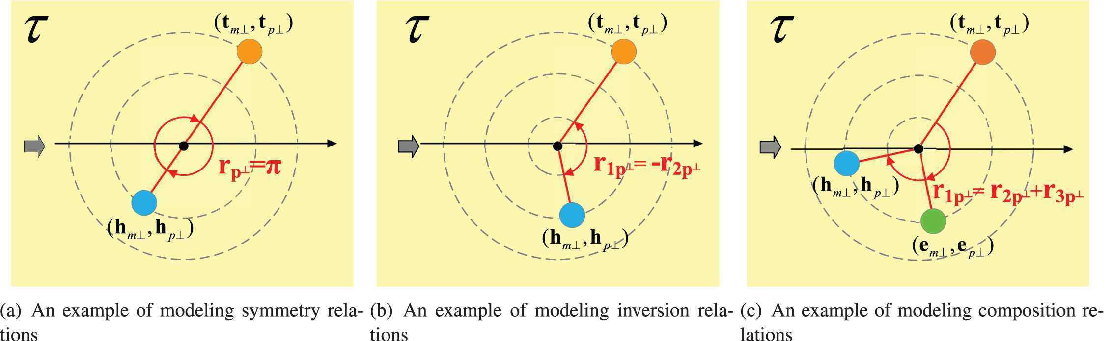
Fig. 5

Scores for facts (Ashley Cole, plays for, {Arsenal F.C. | Chelsea F.C. | A.S. Roma | LA Galaxy}, {[1999-2006] | [2006-2014] | [2014-2016] | [2016-?]}).

4.3Analysis on relation inference

In this part, we show that HTKE could implicitly represent the symmetric relation pattern by analyzing the projected rotation angle of relation embeddings.

The symmetry relation pattern requires the symmetric relation to have each element of its projected rotation angle satisfy [r_p⊥] _i = kπ, k = 0, 1, 2. We investigate the relation embeddings from a 500-dimensional HTKE trained on YAGO11k. Figure 6a gives the distribution histogram of the average angle of each element projected on all time-specific hyperplanes of the symmetric relation embedding ‘isMarriedTo’. We can find that the rotation angles are 0, π or 2π. It indicates that the HTKE does infer and model the symmetry relation pattern. Figure 6b is the histogram of relation ‘wasBornIn’, which shows that the embedding of a general relation does not have such kπ pattern.

Fig. 6

Distribution histograms of two relations embedding phases that reflect the same hierarchy. The x-axis represents the value of entry [r_p⊥] _i, the y-axis represents the number of entry [r_p⊥] _i.

5Conclusion and future work

Temporal knowledge graph (KG) completion is an important problem and has been the focus of several recent studies. We propose a Hyperplane-based Time-aware Knowledge graph Embedding model HTKE for temporal KG completion, which incorporates time information directly to representation space by developing time-specific hyperplanes, and maps facts in the same time-specific hyperplane into a polar coordinate system for modeling and inferring important relation patterns such as symmetry, antisymmetry, inversion and composition. Experiments on three real-world temporal KG datasets show that our model outperforms existing state-of-the-art methods on the KG completion task. Furthermore, our model adapts well to the various time forms of these datasets: points in time, time intervals with beginning and ending. A further investigation shows that HTKE is capable of predicting time scopes for facts with missing time information. In the future, we plan to incorporate type consistency information to further improve our model and also integrate HTKE with open-world knowledge graph completion [49].

References

[1]	Bollacker K. , Evans C. , Paritosh P. , et al., Freebase: a collaboratively created graph database for structuring human knowledge, in: Proceedings of the 2008 ACM SIGMOD international conference on Management of data, 2008, pp. 1247–1250.
[2]	Fabian M. , Gjergji K. , Gerhard W. , et al., Yago: A core of semantic knowledge unifying wordnet and wikipedia, in: 16th International World Wide Web Conference, WWW, 2007, pp. 697–706.
[3]	Miller G.A. , Wordnet: a lexical database for english, Communications of the ACM 38: (11) ((1995) ), 39–41.
[4]	Zhang Z. , Han X. , Liu Z. , et al., Ernie: Enhanced language representation with informative entities, in: Proceedings of the 57th Annual Meeting of the Association for Computational Linguistics, 2019, pp. 1441–1451
[5]	Yasunaga M. , Ren H. , Bosselut A. , et al., Qa-gnn: Reasoning with language models and knowledge graphs for question answering, arXiv preprint arXiv:2104.06378 (2021).
[6]	Wang X. , He X. , Cao Y. , et al., Kgat:Knowledge graph attention network for recommendation, in: Proceedings of the 25th ACM SIGKDD International Conference on Knowledge Discovery & Data Mining, 2019, pp. 950–958.
[7]	Xiong C. , Power R. and Callan J. , Explicit semantic ranking for academic search via knowledge graph embedding, in: Proceedings of the 26th International Conference on world wide web, 2017, pp. 1271–1279.
[8]	Nickel M. , Murphy K. , Tresp V. , et al., A review of relationalmachine learning for knowledge graphs, }(1) 11–, Proceedings of theIEEE 104: ((2015) ), 33.
[9]	Wang Q. , Mao Z. , Wang B. , et al., Knowledge graph embedding: Asurvey of approaches and applications, (12) –, IEEE Transactions onKnowledge and Data Engineering 29: ((2724) ), 2743.
[10]	Nguyen D.Q. , An overview of embedding models of entities and relationships for knowledge base completion, arXiv preprint arXiv:1703.08098 (2017).
[11]	Ward M.D. , Beger A. , Cutler J. , et al., Comparing gdelt and icewsevent data, Analysis 21: (1) ((2013) ), 267–297.
[12]	Leetaru K. and Schrodt P.A. , Gdelt: Global data on events, location, and tone, 1979–2012, in: ISA Annual Convention Vol. 2, Citeseer, 2013, pp. 1–49.
[13]	Mahdisoltani F. , Biega J. and Suchanek F.M. , Yago3: A knowledge base from multilingual wikipedias, 2013.
[14]	Erxleben F. , Günther M. , Krötzsch M. , et al., Introducing wikidata to the linked data web, in: Proceedings of the 13th International Semantic Web Conference-Part I, 2014, pp. 50–65.
[15]	Sun Z. , Deng Z. , Nie J. , et al., Rotate: Knowledge graph embedding by relational rotation in complex space, in: International Conference on Learning Representations, 2018.
[16]	Trouillon T. , Welbl J. , Riedel S. , et al., Complex embeddings for simple link prediction, International Conference on Machine Learning (ICML), 2016.
[17]	Toutanova K. and Chen D. , Observed versus latent features for knowledge base and text inference, in: Proceedings of the 3rd Workshop on Continuous Vector Space Models and their Compositionality, 2015, pp. 57–66.
[18]	Guu K. , Miller J. and Liang P. , Traversing knowledge graphs in vector space, arXiv preprint arXiv:1506.01094 (2015).
[19]	Lin Y. , Liu Z. , Luan H. , et al., Modeling relation paths for representation learning of knowledge bases, arXiv preprint arXiv:1506.00379 (2015).
[20]	Yang B. , Yih W. , He X. , et al., Embedding entities and relations for learning and inference in knowledge bases, arXiv preprint arXiv:1412.6575 (2014).
[21]	Kazemi S.M. and Poole D. , Simple embedding for link prediction in knowledge graphs, in: Proceedings of the 32nd International Conference on Neural Information Processing Systems, 2018, pp. 4289–4300.
[22]	Leblay J. and Chekol M.W. , Deriving validity time in knowledge graph, in: Companion Proceedings of the The Web Conference 2018, 2018, pp. 1771–1776.
[23]	Lacroix T. , Obozinski G. and Usunier N. , Tensor decompositions for temporal knowledge base completion, arXiv preprint arXiv:2004.04926 (2020).
[24]	Dasgupta S.S. , Ray S.N. and Talukdar P. , Hyte: Hyperplane-based temporally aware knowledge graph embedding, in: Proceedings of the 2018 Conference on Empirical Methods in Natural Language Processing, 2018, pp. 2001–2011.
[25]	Garcia-Duran A. , Dumančić S. and Niepert M. , Learning sequence encoders for temporal knowledge graph completion, in: Proceedings of the 2018 Conference on Empirical Methods in Natural Language Processing, 2018, pp. 4816–4821.
[26]	Ma Y. , Tresp V. and Daxberger E.A. , Embedding models for episodicknowledge graphs, , Journal of Web Semantics 59: ((2019) ), 100490.
[27]	Goel R. , Kazemi S.M. , Brubaker M. , et al., Diachronic embedding fortemporal knowledge graph completion, in: Proceedings of theAAAI Conference on Artificial Intelligence 34: (2020) , pp. 3988–3995.
[28]	Kazemi S.M. , Goel R. , Jain K. , et al., Representation learning fordynamic graphs: A survey, Journal of Machine Learning Research 21: (70) ((2020) ), 1–73.
[29]	Ji S. , Pan S. , Cambria E. , et al., A survey on knowledge graphs: Representation, acquisition and applications, arXiv preprint arXiv:2002.00388 (2020).
[30]	Li B. and Pi D. , Network representation learning: a systematic literature review, Neural Computing and Applications (2020), 1–33.
[31]	Bordes A. , Usunier N. , Garcia-Duran A. , et al., Network representation learning: a systematic literature review, Neural Computing and Applications (2020), 1–33.
[32]	Zhang Z. , Cai J. , Zhang Y. and Wang J. , Translating embeddings for modeling multi-relational data, in: Advances in Neural Information Processing Systems, 2013, pp. 2787–2795.
[33]	Liu H. , Bai L. , Ma X. , Yu W. and Xu C. , Projfe: Prediction of fuzzyentity and relation for knowledge graph completion, , Applied Soft Computing 81: ((2019) ), 105525.
[34]	Lacroix T. , Usunier N. and Obozinski G. , Canonical tensor decomposition for knowledge base completion, in: Proceedings of the 35th International Conference on Machine Learning, PMLR, 2018, pp. 2863–2872.
[35]	Hitchcock F.L. , The expression of a tensor or a polyadic as a sum ofproducts, Journal of Mathematics and Physics 6: (1-4) ((1927) ), 164–189.
[36]	Balažević, I. , Allen C. and Hospedales T.M. , Tucker: Tensor factorization for knowledge graph completion, arXiv preprint arXiv:1901.09590 (2019).
[37]	Tucker L.R. , Some mathematical notes on three-mode factor analysis, Psychometrika 31: (3) ((1966) ), 279–311.
[38]	Montella S. , Rojas-Barahona L. and Heinecke J. , Hyperbolic temporal knowledge graph embeddings with relational and time curvatures, arXiv preprint arXiv:2106.04311 (2021).
[39]	Chami I. , Wolf A. , Juan D.-C. , Sala F. , Ravi S. and Ré C. , Low-dimensional hyperbolic knowledge graph embeddings, in: Proceedings of the 58th Annual Meeting of the Association for Computational Linguistics, 2020, pp. 6901–6914.
[40]	Jung J. , Jung J. and Kang U. , Learning to walk across time for interpretable temporal knowledge graph completion, in: Proceedings of the 27th ACM SIGKDD Conference on Knowledge Discovery & Data Mining, 2021, pp. 786–795.
[41]	Gracious T. , Gupta S. , Kanthali A. , Castro R.M. and Dukkipati A. , Neural latent space model for dynamic networks and temporalknowledge graphs, in: Proceedings of the AAAI Conference onArtificial Intelligence 35: ((2021) ), 4054–4062.
[42]	Zhu C. , Chen M. , Fan C. , Cheng G. and Zhang Y. , Learning fromhistory: Modeling temporal knowledge graphs with sequentialcopy-generation networks, in: Proceedings of the AAAIConference on Artificial Intelligence 35: ((2021) ), 4732–4740.
[43]	Han Z. , Chen P. , Ma Y. and Tresp V. , Explainable subgraph reasoning for forecasting on temporal knowledge graphs, in: International Conference on Learning Representations, 2021.
[44]	Bai L. , Ma X. , Zhang M. and Yu W. , Tpmod: A tendency-guidedprediction model for temporal knowledge graph completion, ACMTransactions on Knowledge Discovery from Data 15: (3) ((2021) ), 1–17.
[45]	Bai L. , Yu W. , Chen M. and Ma X. , Multi-hop reasoning over paths intemporal knowledge graphs using reinforcement learning, , {AppliedSoft Computing 103: ((2021) ), 107144.
[46]	Bordes A. , Usunier N. , Garcia-Duran A. , et al., Irreflexive and hierarchical relations as translations, arXiv preprint arXiv:1304.7158 (2013).
[47]	Adam P. , Sam G. , Soumith C. , et al., Automatic differentiation in pytorch, in: Proceedings of Neural Information Processing Systems, 2017.
[48]	Kingma D.P. and Ba J. , Adam: A method for stochastic optimization, arXiv preprint arXiv:1412.6980 (2014).
[49]	Shi B. and Weninger T. , Open-world knowledge graph completion, Association for the Advancement of Artificial Intelligence, (2018).