Robust adaptive fuzzy control design for nearspace vehicle
Abstract
In this paper, a T-S fuzzy model of the NSV (Nearspace Vehicle) kinematic model is established based on fuzzy approximation theory, and a new fuzzy robust tracking control law is designed in reference to the feedforward control of the linear system. In order to account for a case in which no augmented matrix is introduced, the control law is designed as a compound form of feedback and feedforward, and the gains of feedback and feedforward are solved by LMI (Linear Matrix Inequalities). The strategy is applied to the anti-interference control of NSV attitudes, and the convergence of tracking errors is analyzed according to the Lyapunov method. Simulation results based on the NSV demonstrate the validity of the proposed method.
1Introduction
It is well known that the fuzzy control technique provides a means of collecting knowledge and expertise. Over the past decade, it has proved to be very useful in many applications [8, 10, 13, 14, 19]. It is not surprising that T-S fuzzy models have become one of the most useful control approaches for complex nonlinear systems. Many nonlinear systems can be represented by T-S fuzzy systems, allowing designers to take advantage of conventional linear system methods to for design and analysis [2, 4, 6, 7, 18, 21, 22]. The fuzzy adaptive control can not only automatically adjust to control rules in the face of change in performance and parameters of the controlled object, but also enhance the adaptive ability to deal with environmental changes and realize the purpose of control.
The control design of NSVs has attracted increasing attention in recent years. The primary reason is that they have potential and promising applications in both military and civilian fields. Since a Nearspace vehicle is a complex dynamic system, it is difficult to study according to traditional control methods. To overcome this limitation, a T-S fuzzy control scheme has been considered to cope with such problems. The major advantage of this scheme is that an accurate mathematical model is not necessary, and consequently, the T-S fuzzy control theory is suitable for the design of the flight control system of an NSV [5, 15]. However, the Nearspace hypersonic vehicle dynamics are severely nonlinear, time-varying, highly uncertain and strongly coupled. It also suffers from different external disturbances and uncertainties due to changes in the flight environment. Therefore, ensuring the robust stability of the NSV flight is challenging. To date, this subject has not been fully investigated.
This paper proposes the design of a feedback and feedforward control for T-S fuzzy systems, which has been applied to the tracking control of attitude angle of the NSV. The organization of the paper is as follows: Section 2 describes design formulation. Section 3 describes the tracking controller design of the NSV, and presents the design of an anti-interference composite controller, as well as the calculation method of feedforward gain and feedback gain by LMI. The simulation results which demonstrate the effectiveness of the proposed approaches are presented in Section 4, followed by conclusions in Section 5.
2Problem formulation
The mathematic model of the NSV developed at NASA (National Aeronautics and Space Administration) Langley Research Center is given asfollows:
(1)
where α is the angle of attack, β is the sideslip angle, μ is the bank angle, p is the roll rate, q is the pitch rate and r is the yaw rate.
According to singular perturbation theory, the six equations can be divided into the fast loop and the slow loop, respectively. The above attitude motion equations can thus be rewritten as follows:
(2)
(3)
According to the following: x(t) = [ω(t)T, Ω(t)T], u(t) = TC , y(t) = ω(t) system (2) can also be represented as follows:
(4)
3The tracking controller design for NSV
3.1Stability analysis
In recent years, many important results regarding stability analysis for T-S fuzzy control systems have been reported [1, 3, 5, 9, 15]. In this section, the following T-S fuzzy model of the NSV is considered, and which is composed of a set of fuzzy implications. The ith rule of this T-S fuzzy model is of the following form. Then, based on the Lyapunov stability theorem, a sufficient condition is derived in terms of LMIs, which can guarantee the stability of the closed-loop control system.
(5)
According to fuzzy principles, system (5) can be described as follows:
(6)
For all t, therefore:
Nij (z (t)) is the grade of membership of Nik.
For a dynamic system, the feedback controller can be represented as follows:
(7)
The H∞ gain is defined for the system anti-interference characteristics as follows:
(8)
Theorem 1. Considering system (6), for i, j = 1, 2, … , r, Ei and Ej are the known real constant matrices of appropriate dimensions. If rate of decay λ and a symmetric positive definite matrix P exist, then any set of state feedback control gains Kj must meet the following matrix inequality:
(9)
Proof. Choose the Lyapunov function candidate
(10)
The time derivative (10), the following is obtained:
Integrating both sides with respect to time:
Due to V ( x (t)) ≥0, then
Therefore
3.2The robust controller design
In order to design a control law to guarantee the stability of the closed-loop system and to eliminate the effect of external disturbances and uncertainties. the composite controller of NSV, system (4), can be described as follows:
(11)
(12)
In accordance with T-S fuzzy theory, the control rules can be designed as follows:
(13)
In order to prove the stability of the track, the following lemma is given.
Lemma 1. [17] Let
X be a symmetric matrix given by:
The following conditions are equivalent:
(i) X < 0
(ii) X11 < 0 and
(iii) X22 < 0 and
Assumption 1. There exists a known bounding matrix Ξπ satisfying ∥ψ (t)∥ ≤ ∥ Ξπ ∥, where ψ (t) is the external disturbance in system (11).
Assumption 2. There exists a known bounding matrix Ξ such as ∥ d ( x (t))∥ ≤ ∥ Ξ ∥, where d ( x (t)) is the unknown bounded uncertainty in system (11).
Based on the above analysis, the robust adaptive control of the vehicle can be surmised according to the following theorem.
Theorem 2. For i, j = 1, 2, ⋯ , r, there exists a real symmetric positive definite matrix P, which satisfy the following the inequality.
(14)
Theorem 3. For i, j = 1, 2, …, r, ( D, Fj) satisfying condition
(15)
According to the solutions of ( D, Fj), the feedforward control gains Kcj are obtained.
4Simulation
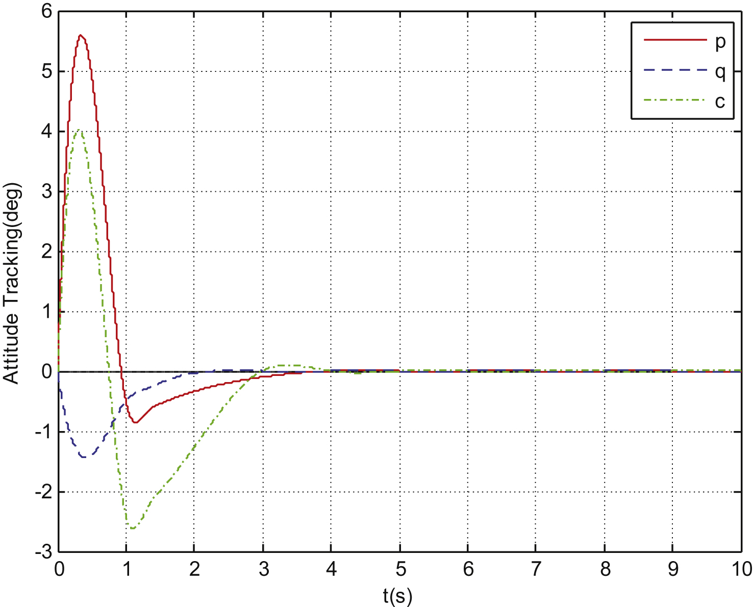
In this section, simulation results are presented in order to illustrate the effectiveness of the proposed robust control scheme. Considering the nonlinearity of NSV dynamics, the aerodynamic coefficients are taken as the nominal cruising flight; the nominal flight of an NSV occurs at a trimmed cruise condition (V = 2500 m/s, H = 45 km); the initial attitude angle conditions are chosen as α = 1°, β = -1°, μ = -1°; the body-axis angular rate is assumed to be p = q = r = 0°/s; the reference commands are αc = 3 .4°, βc = 0°, and μc = 1 .2°, respectively. The external disturbance of the NSV system is 2 × 10⁵ · [sin(2t) , sin(2t) , sin(2t)] T Nm, and the system exists – 20% aerodynamic parameter perturbation.
According to Theorem 2, the feedback control gains Kj can be obtained as follows:
The reference model is given as follows:
In Theorem 3, Kcj = Fj - Kj D were obtained.
The simulation results indicate the following conclusions. Figure 1 depicts the tracking curve of the angle of attack α; Fig. 2 represents the tracking curve of the sideslip angle β; Fig. 3 depicts the tracking curve of the bank angle μ; and Fig. 4 shows the p, q, r state response curve (p is the roll rate, q is the pitch rate and r is the yaw rate.). The variables αc, βc, μc are the reference commands of attitude angle α, βμ, respectively.
As shown in Figs. 1 through 4, the closed-loop system is asymptotically stable under the proposed robust compound controller. Thus, the proposed fuzzy control scheme based on feedback control and feedforward control is validated.
5Conclusion
T-S fuzzy control schemes have been developed for the NSV system with functional uncertainty and external disturbance. Feedforward and feedback composite control is adopted to eliminate the external disturbance of the NSV. The controller design has been implemented in a unified manner in which gains are solved according to a set of LMIs. Simulation results have demonstrated the effectiveness of the proposed model. NSV is a complex dynamic system; future work will take random factors and stochastic noises in developments of NVS models into accountance [11, 12, 16], and will study attitude tracking control and accommodation approaches to NSVs with functional uncertainty and external disturbance.
Acknowledgments
The authors wish to thank the editor and anonymous reviewers for useful comments and suggestions, especially for Mr. Bryn Jones who is a British gas turbine combustion specialist. This work is partially supported by JSUT Research Funding (Granted Numbers: KYY13001 and KYY13017), Foundation items: The Natural Science Foundation of Jiangsu Province (BK2012584 and BK20130234), Chang Zhou Science and Technology Support Program (CE20145056) and Innovation Team Funding (Granted Number: TDZD13003).
References
1 | Kole A (2015) Design and stability analysis of adaptive fuzzy feedback controller for nonlinear systems by Takagi–Sugeno model-based adaptation scheme Soft Computing 19: 6 1747 1763 |
2 | Peng C, Han QL, Yue D, Tian E (2011) Sampled-data robust H (∞) control for T–S fuzzy systems with time delay and uncertainties Fuzzy Sets and Systems 179: 1 20 33 |
3 | Huang CP (2014) Stability analysis and controller synthesis for discrete uncertain singular fuzzy systems with distinct difference matrices in the rules Internat J Systems Sci 45: 9 1830 1843 |
4 | Jiang CS, Wu QX, Fei SM (2012) Harbin Institute of Technology Press, Harbin Modern Nonlinear Robust Control System |
5 | Chen GY, Ning L, Li SY (2010) The stability of a class of T-S fuzzy control system analysis and design Control Theory and Application 27: 3 310 316 |
6 | Škrjanc I, Blažič S, Matko D (2002) Direct fuzzy model-reference adaptive control International Journal of Intelligent Systems 17: 10 943 963 |
7 | Dong JX, Wang YY, Yang GH (2011) H (∞) and mixed H (2)/H (∞) control of discrete-time T–S fuzzy systems with local nonlinear models Fuzzy Sets and Systems 164: 1 1 24 |
8 | Chen M, Jiang CS, Wu QX (2011) Disturbance-observer-based robust flight control for hypersonic vehicles using neural networks Advanced Science Letters 4: 1771 1775 |
9 | Meda-Campana JA, Rodriguez-Valdez J, Hernandez-Cortes T, Tapia-Herrera R (2015) Analysis of the fuzzy controllability property and stabilization for a class of T-S fuzzy models IEEE Transactions on Fuzzy Systems 23: 2 291 301 |
10 | Chang MK, Liou JJ, Chen ML (2011) T–S fuzzy model-based tracking control of a one-dimensional manipulator actuated by pneumatic artificial muscles Control Engineering Practice 19: 12 1442 1449 |
11 | Malinowski MT, Agarwal RP (2013) Some properties of strong solutions to stochastic fuzzy differential equations Information Sciences 252: 62 80 |
12 | Malinowski MT, Agarwal RP (2015) On solutions to set-valued and fuzzy stochastic differential equations Journal of the Franklin Institute 352: 3014 3043 |
13 | Shen Q, Jiang B, Cocquempot V (2012) Fault-tolerant control for T–S fuzzy systems with application to near-space hypersonic vehicle with actuator faults IEEE Transactions on Fuzzy Systems 20: 4 652 665 |
14 | Zhou Q, Li HY, Shi P (2015) Decentralized adaptive fuzzy tracking control for robot finger dynamics IEEE Transactions on Fuzzy Systems 23: 3 501 510 |
15 | Precup RE, Tomescu ML, Preit S (2009) Fuzzy logic control system stability analysis based on Lyapunov’s direct method International Journal of Computers, Communications & Control 4: 4 415 426 |
16 | Yacoub RR, Riyanto T, Bambang A, Harsoyo J (2014) Sarwono, DSP implementation of combined FIR-functional link neural network for active noise control International Journal of Artificial Intelligence 12: 1 36 47 |
17 | Boyd S, Ghaoui LE, Feron E (1994) Linear Matrix Inequalities in System and Control Theory, SIAM, Philadelphia |
18 | Senthilkumar T, Balasubramaniam P (2011) Robust H (∞) control for nonlinear uncertain stochastic T–S fuzzy systems with time delays Applied Mathematics Letters 24: 12 1986 1994 |
19 | Wang YH, Wu QX, Jiang CS (2009) Reentry attitude tracking control based on fuzzy feedforward for reusable launch vehicle International Journal of Control, Automation, and on Systems 7: 4 503 511 |
20 | Chen ZF, Aghakhani S, Man J, Dick S (2011) ANCFIS: A neurofuzzy architecture employing complex fuzzy sets IEEE Transactions on Fuzzy Systems 19: 2 305 322 |
21 | Yu ZJ, Xu YN (2014) Research of adaptive fault-tolerant control based on T-S fuzzy model International Journal of Modeling and Optimization 4: 1 62 66 |
Figures and Tables
Fig.1
Angle of attack α tracking curve.
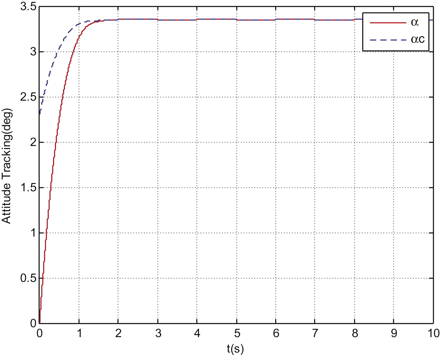
Fig.2
Sideslip angle β tracking curve.
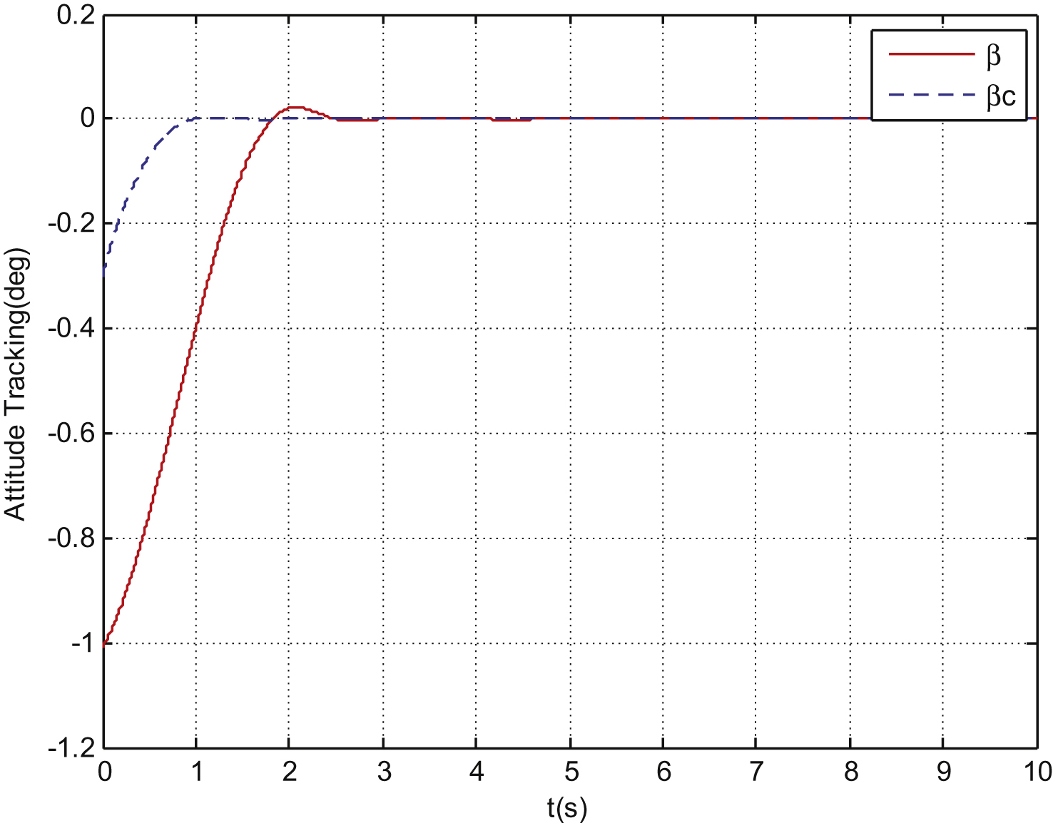
Fig.3
Bank angle μ tracking curve.
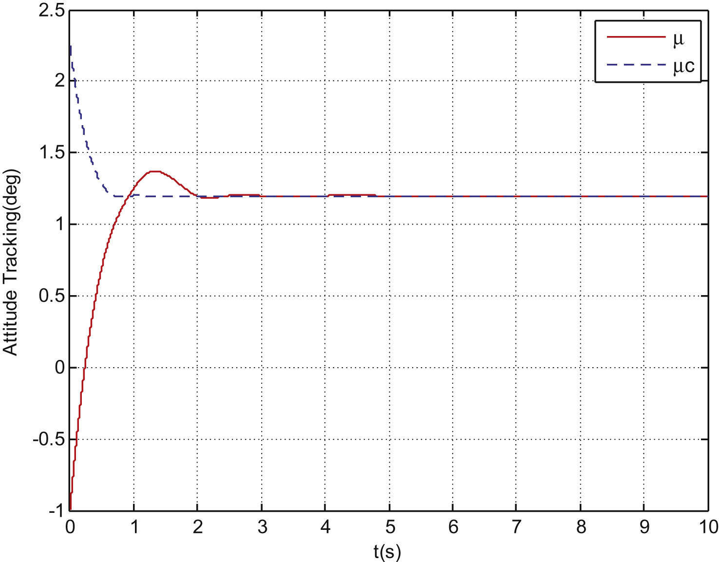
Fig.4
Angular rate p, q, r state response curve.