
Attitude control based on fuzzy logic for continuum aircraft fuel tank inspection robot
Abstract
With a compliant structure and excellent bending properties, continuum robot has hyper-redundant degrees of freedom, and can be used in space-constrained environments as the aircraft fuel tank. Therefore, a continuum robot is designed to help crews inspect aircraft fuel tanks, which can improve maintenance efficiency and reduce the intensity of crews. According to the requirements of aircraft fuel tank inspection, the compliant and extensible drive mechanisms of the continuum robot are designed. The kinematic models of single joint segment and multi-joint segments of continuum robot are analyzed, and homogeneous transformation matrices are obtained. To improve control performance, a closed-loop fuzzy controller based on attitude feedback is proposed. The attitude sensor is installed on the top of each joint segment of a snake-like arm to form a closed-loop control system, and a fuzzy controller is designed to achieve fast and accurate control of the robot. The prototype platform of the continuum robot is built, and practical experiments are implemented on the platform. The effectiveness and stability of the fuzzy controller based on attitude feedback are verified.
1Introduction
Currently, inspections of fuel tanks in civil aviation are primarily performed manually during aircraft maintenance, and the crews often have to enter the fuel tank for inspection. As the operating space in the tank is small and it is difficult to determine the position of leakages and corrosions, the checking efficiency is low. Furthermore, a tank with fuel vapor inside is a flammable and explosive environment, posing a threat to the health of the crews.
A continuum robot has redundant degrees of freedom, can move flexibly and has a large workspace. Thus, the robot has structural advantages whenworking within strict space constraint. This paper presents a design for an aircraft fuel tank inspection robot (AFTIR) with a continuous structure to assist crews in conducting efficient and risky fuel tank inspection operations.
Several research teams have studied topics related to continuum robots, mostly applied to the medical field, particularly for minimally invasive surgery (MIS). Continuum robots designed to enter a given operative position have been proposed in previous studies [10, 11]. These robots were driven by cables. Kinematics models have been built and analyzed. The approach for compliant motion control that does not require explicit estimation of interaction forces has also been presented in previous studies [1, 2]. A continuum robot with a coupled tendon drive has been developed for use in the examination of human heart disease [4]. The authors presented a method of controlling a tendon-driven continuum manipulator by specifying the shape configuration. The basis for the control was a linear beam configuration model that transformed the beam configuration into tendon displacement by modelling the internal loads of the compliant system [5]. In previous studies based on the analysis of continuum robots, a novel and simplified kinematics for cable-driven continuum robots was presented using geometric analysis [8, 9]. The mapping relationships between simple joint drive space, joint space, and operation space were analyzed, and the 3D workspace wasintroduced.
In order to make continuum robots perform tasks, improvements to control performance indices are necessary, such as the control accuracy of endpoint. Open-loop control mode is adopted in traditional control of continuum robots, and the control performance depends on building complex kinematics and dynamics models. At present, some scholars have studied the feedback of the flexible mechanism of continuum robot. Yoel Shapiro [14, 15] and others have designed a continuum robot whose shape can be measured with several film piezoelectric polymer deflection sensors consisting of polyvinylidene fluoride (PVDF). With the bending feedback of the flexible arm, a closed-loop controller was adopted and control accuracy was improved. Beobkyoon Kim [3], Seok Chang Ryu [13] etc. designed a project in which a 3D space shape of a continuum robot was achieved based on the optical sensor feedback of fiber bragg grating (FBG) to implement the closed-loop control of a flexible manipulator.
Worldwide, there are fewer reports in the study of aircraft fuel tank inspection robots. The robotics institute of Civil Aviation University of China have conducted sustaining research, and created an experimental prototype system with the continuous structure [6]. The inspecting portion of the system entering the fuel tank was the continuous snake arm, and a cable-driven control mode was adopted. Wang Lei, et al. [12] researched the path-planning problem in the tank inspection by a continuum robot, and a path-planning algorithm based on goal orientation was imposed. The path-planning algorithm based on a projection strategy was proposed for aircraft fuel tanks under obstacle environment [7]. However, the robot was controlled by an open-loop mode, resulting in less control precision.
In summary, in order to improve the control performance of a continuum robot, there are typically two methods: (1) establish accurate kinematic and dynamic models; (2) design a closed-loop feedback control system. Due to the high complexity of the continuum robot modeling, the design of closed-loop system is adopted to obtain better control precision in this paper.
2Mechanism design of AFTIR
Considering the environmental features of aircraft fuel tanks, a flexible continuous structure is used in the design of AFTIR, primarily composed of a mobile platform, a telescopic mechanism, a snake-like arm mechanism (SLA), a drive mechanism and a control unit, as shown in Fig. 1. It is easy to realize the free movement of the robot by a mobile platform.
The telescopic mechanism includes a linear module and a DC motor, and can provide one degree of freedom to realize translation motions of the SLA which must enter or exit the aircraft fuel tank. The SLA is a carrier for entering the fuel tank in order to perform inspection operations, with redundant degrees of freedom. The drive mechanism provides power for movement of the SLA. The control unit is the core of the system, primarily consisting of the main control computer, motion control cards and drive cards, sensor acquisition modules, etc., to achieve the movement planning and control functions of the SLA. The core design of the system structure is the SLA mechanism, and the design details are as follows:
The SLA mechanism is composed of a series of several joint segments (JS). The shape of the SLA is cylindrical and demonstrates excellent bending performance. The cable-driven mode is used to drive the SLA. Each JS consists of a flexible backbone, a base disc, an end disc, several support discs, and three driving cables, as shown in Fig. 2. The base disc, the end disc and several support discs are connected by the flexible backbone at their centers, so that the motion characteristics are governed by elastic deflections of the backbone. For 2-DOF JS, the flexible backbone is comprised of carbon fiber rods, and its structure is designed so that it possesses a very high tensional stiffness to prevent twisting around the backbone axis. As a result, the JS with the flexible backbone will only produce 2-DOF motions. To simplify SLA analysis, all JSs are assumed to be identical. The attachment points of the three driving cables are symmetrically arranged at 120°on both discs. Each drive cable is controlled by one motor.
3Kinematic analysis of AFTIR
3.1Kinematic analysis of single JS
The SLA of AFTIR is composed of several JSs, and each JS has identical characteristics; therefore, the first JS of SLA is taken as an example for kinematic analysis. The base frame {1} and the end frame {2} are separately established based on the disc center o 1 and o 2. The z 1 axis of frame {1} and z 2 axis of frame {2} are respectively perpendicular to the circumference plane of the discs, and point to the tangent direction of the JS.
The movement of the JS is driven by three cables, and can be decomposed into bending movement and rotational movement, rotating by axis z 1, respectively designated as the bending DOF and rotational DOF.
The kinematic model of the single JS is shown in Fig. 3. The curve of the JS is a continuous smooth curve with equal curvature, and the bending angle is a central angle θ corresponding to the bending arc, ranging from 0 to π. The rotation angle is φ, which is the angle between the plane oo 1 o 2 and plane x 1 o 1 z 1, ranging from 0 to 2π. As terminal coordinates and attitudes of the JS are determined by θ and φ, so θ and φ are called joint variables.
The homogeneous transfer matrix T of frame {2} with respect to {1} can be described by Formula (1).
(1)
3.2Kinematic analysis of multi-JS
The nearest JS of the base is the first JS(JS1), followed by the second JS (JS2), the third JS (JS3), etc. Frame {n } (n = 1, 2, 3, 4, ⋯) at the center of the base disc of each JS is established, and frame {n + 1 } (n = 1, 2, 3, 4, ⋯) at the center of the end disc of each JS is also established. The z n axis of frame {n} is perpendicular to the disc. Since the end disc of each JS is connected to the base disc of the next JS, the two coordinates can be considered coincidental.
The bending angle and the rotation angle of the n-th JS are defined as (θ n , φ n ), and the homogeneoustransformation matrix from frame {n + 1} to frame {1} is expressed as:
(2)
3.3Mapping from joint space to drive space
The flexible SLA of the continuum robot is controlled by drive cables. Therefore, it is necessary to calculate the length variation of drive cables, and the mapping from the joint space to the drive space must be analyzed.
The backbone of the SLA is made of a carbon fiber rod, and the bending model can be approximated as an arc with equal curvature. While the drive cables through the discs are shown in a polyline state when the SLA bends, errors of drive cables in each JS will be accumulated.
The bending angle of a single JS is θ, and the rotation angle is φ. The bending model is shown in Fig. 4. The drive cables between adjacent discs are polylines; because the discs are equally spaced, the lengths of these polylines are identical. The lengths of a single-segment polyline can be calculated by Equation (3) through a geometric relationship.
(3)
Through the geometric relationships, these equations are obtained as follows:
(4)
(5)
(6)
Equation (7) can be obtained from Equations (3) through (6).
(7)
Assume that the SLA is comprised of N (N ≥ 1) joint segments, and the threading holes are numbered counterclockwise. The distribution is shown in Fig. 5, and the angle between two adjacent holes is represented by α.
(8)
The joint variables of the i# joint are set as (θ i , φ i ), and the cable length variation ΔL ij of the drive cable which threads the j# hole is expressed as follows:
(9)
When the multiple JS move, the length variation of each drive cable in each segment must be calculated; then, the total length variation
(10)
4The design of fuzzy controller based on attitude feedback
4.1Attitude feedback system design of continuum robot
A predetermined position of the SLA can be obtained by changing the length of the drive cables according to fit the established SLA model of continuum AFTIR. However, the position control error of the SLA may be very large according to the influence of such factors as transmission error, the different tensile strengths of drive cables, or inaccurate control models. Therefore, a fuzzy logic controller based on attitude feedback is designed, to improve system reliability and accuracy of position control.
When the SLA is bending, the frame attitude of the end JS can be represented by joint variables, and a definite function can be found between the end position of the JS and joint variables. Therefore, a position closed-loop controller of the SLA is proposed with the end attitude of JS serving as feedback.
A 9-axis inertial navigation module JY - 901 is adopted to measure the attitude of the SLA. Dynamics calculation and a dynamic kalman filter algorithm are realized using a high-performance microprocessor, and can quickly solve the attitude angle in real time.
4.2Attitude angle transformation
The rotation transformation of the end coordinate system relative to the base is in accordance with Z-Y-Z order based on the model of single JS. However, attitude angles measured by the sensor are RPY angles, which represent Euler angles by Z-Y-X rotation orders. Therefore, it is necessary to convert Euler angles of ZYX to ZYZ angles as current joint variables of SLA are demanded to achieve a closed-loop control.
The transformation of coordinate systems can be achieved by the rotation of different orders, so that the rotation transformation matrices are the same. ZYX Euler angles, measured by the attitude sensor, can be used to solve the transformation matrix, and then ZYZ Euler angles can be determined.
Define ZYX Euler angles of a coordinate transformation for (ω, ξ, ψ); the corresponding relationship to RPY angles is as follows:
(11)
The rotational transformation matrix can be obtained as follows:
(12)
Set ZYZ Eeuler angles of a coordinate transformation for (α, β, γ); the rotation transformation matrix is as follows:
(13)
Let R (α, β, γ) = R (ω, ξ, ψ), and then ZYZ Euler angles (α, β, γ) can be calculated. For simplicity, R (ω, ξ, ψ) can be written as follows:
(14)
When sβ ≠ 0, ZYZ Euler angles (α, β, γ) can be calculated as follows:
(15)
When β = 0°, ZYZ Euler angles (α, β, γ) can be determined as follows:
(16)
When β = 180°, ZYZ Euler angles (α, β, γ) can be determined as follows:
(17)
The rotation angles by ZYZ axes at the end JS coordinate system relative to the head coordinate system are (φ, θ, - φ). By analyzing the kinematics model of a single JS, they fulfill the following equation:
(18)
The angle should satisfy the relationship as presented in Equation (18):
(19)
As the angle of ω as measured by attitude sensors is easily influenced by the initial magnetic field calibration and environmental magnetic field, it can lead to large measuring error, and the accuracy is reduced in solving for α. However, the measurement accuracy is higher when disregarding ω when solving β and γ; therefore, (β, - γ) is employed as feedback for joint variables (θ, φ) in the attitude control of a single JS.
4.3The design of fuzzy controller
The traditional PID control algorithm has less capability to achieve rapid accuracy during the entire workspace (for each JS, the range of bending angle is [0, π], and the range of rotation angle is [0, 2π). The fuzzy control can be adjusted to the control in a wide range based on fuzzy control rules. Therefore, fuzzy logic control is used to improve the dynamic and steady performance of the SLA control.
Figure 6 shows the control block diagram of a fuzzy controller based on attitude feedback of a single JS.
Desired joint angles (θ, φ) of the JS are used as the system inputs, and the end attitudes of JS as measured by attitude sensors are used as feedback signals, which have been converted to joint variables by Euler angle transformations. The drive cable length deviation e L is obtained by analyzing the difference between the system inputs and feedback signals in the kinematic model of JS. Then, the fuzzy controller is designed as follows:
(1) Determine input and output of fuzzy controller
A 2-D fuzzy controller is adopted; input variables of the fuzzy controller are the maximum value of the deviation e Lmax among deviations e L of three drive cables and the maximum amount of deviation variation de Lmax/dt, and the output of the fuzzy controller is the speed of the drive cable v.
According to the bending and rotation ranges of JS, the range of drive cable deviation e Lmax is defined as [–5 mm, 5mm], the range of the drive cable deviation variation is defined as [–4 mm/s, 4 mm/s], the range of drive cable speed is defined as [–4 mm/s, 4 mm/s].
(2) Design of fuzzy control rules
(a) Design of fuzzy variable
Define fuzzy variables error E, error variation EC and output U, corresponding to the fuzzy controller inputs and output. Their ranges are all defined as { - 3, - 2, - 1, 0, 1, 2, 3}. The values of the fuzzy variables are all defined as follows:
{NB, NM, NS, ZO, PS, PM, PB}.
(b) Define membership functions of linguistic values
The triangle membership function is chosen to express all of the language variables including error E,error variation EC and output U,as shown in Fig. 7.
(c) Fuzzy reasoning method
Fuzzy logic control is a computer-controlled system based on fuzzy set theory, in which the experience of skilled operators and the knowledge of experts are summed up into the control rules in the form of “IF…THEN…”.
The designed fuzzy control rules are shown in Table 1. The Mamdani fuzzy reasoning algorithm is adopted to compute the output of the fuzzy controller.
(3) Defuzzification
The area centroid method is used to conduct defuzzification of output variables.
Quantization factors and scale factors are used during the translation of universes. Quantization factors k e and k ec are used to transform the inputs of the fuzzycontroller from the basic universe into the fuzzy universe; the scale factor k u is used to transform the output from the fuzzy universe to the basic universe. The values of k e , k ec and k u are 0.07, 0.75 and 1.33, respectively.
The velocity of each drive cable is adjusted by a strategy with equal running time for each drive cable of a single JS. The velocity of the drive cable as solved by the fuzzy controller is the maximum value of the three drive cables of a single JS, then set as the velocity of the maximum deviation of the drive cables. The velocities of other drive cables are solved according the principle of equal time.
5Control experiments of AFTIR
In order to verify the fuzzy control effect of a continuum robot based on attitude feedback, a prototype platform with two segments is designed and built, as shown in Fig. 8. The SLA is composed of two JSs. Lengths of both JSs are identical at 250 mm, and the diameters are 35 mm (JS1) and 30 mm (JS2). A JY-901 attitude sensor and three IM-S-1-C10 film pressure sensors are fixed to the end of each JS.
The tension of each drive cable is detected by the control system in real time, and the limit control is implemented. When the tension is lower than the set minimum value, the drive cable will be pulled; when the tension is greater than the set maximum value, the drive cable will be relaxed. Drive cables of the SLA are neither loose nor excessively tight in the movingprocess according to the tension limit control of the drive cables, ensuring reliable operation of the SLA.
In order to verify the fuzzy controller, the experiments are conducted as follows. The SLA is controlled to conduct a bending motion as shown in Table 2, separately conducted for two cases. One case is tested in the absence of attitude feedback, and one is conducted with feedback. The initial bending angle of the SLA in each experiment is 0°, and the attitude angles of the sensors are recorded before and after the attitude correction. For convenience of the experiment, the rotation angles of the SLA are set to 0. Since JS2 bends on the basis of JS1, when the two joint segments move in the same plane, the attitude angle measured by the sensor of JS2 represents the sum of the actual bending angles of the two joints.
Experimental results indicate that a large angle error will be caused by a system model, transmission error and other factors without feedback, and that the error will increase with an increase in the bending angle. However, the set angle can be reached accurately with feedback control, with a steady error less than 0.5°.
The fifth experiment in Table 2 is taken as an example to study the dynamic response during the control process, and the response curve is shown in Fig. 9.
Figure 9(a) shows the curves of bending angles of two segments by fuzzy control and PID control algorithms, respectively, where parameter tuning of the PID regulator had been done as accurately as possible. The attitude angles of JS2 represent the sum of the actual bending angles of the two joint segments. Compared to PID control, fuzzy control can decrease the overshoot and the transient time; the details are shown in Table 3. The velocity change curves of each drive cable in two joints by fuzzy control method are respectively described in Fig. 9(b) and (c). The output of the fuzzy controller is the maximum velocity of the drive cables in each JS, and then other velocities of drive cables are solved according to the velocity control strategy. Figure 9 demonstrates that the output velocity is large and the rise time is short when the angle error is large. When the feedback angle is close to the setting angle, the output velocity reduces.
Experimental results indicate that adjusting the drive cable velocity by the fuzzy controller can obtain good dynamic response and a small steady error.
Experimental figures of groups 1–4 in Table 2 are shown in Fig. 10. The background curves are drawn at a ratio of 1:1, and demonstrate that the center line of the SLA can be well coincided to the theoretical curves.
The experiments verify that the fuzzy control based on attitude feedback demonstrates good control effect, and can rapidly and accurately drive the SLA to reach the setting position.
6Conclusion
A continuum robot used for aircraft fuel tank inspection is designed, and a cable-driven remote control mode is adopted. A flexible mechanism of the robot is designed. In order to improve the accuracy of SLA control, a closed-loop fuzzy control method based on attitude feedback is proposed. An attitude sensor is installed on the top of each JS of the SLA to form a closed-loop control system. The velocity of cables can be adjusted online by the designed fuzzy rule base in order to achieve fast and accurate control. A prototype platform of the continuum robot is built to implement the motion control experiment of two joint segments, and results verify the rapidity and accuracy of fuzzy control based on attitude feedback.
Acknowledgments
This work has been funded by Tianjin Research Program of Application Foundation and Advanced Technology (Youth Foundation #14JCQNJC04400). The supports by Robotics Institute of Beihang University and Robotics Institute of Civil Aviation University of China are acknowledged.
References
1 | Bajo A, Simaan N (2012) Kinematics-based detection and localization of contacts along multisegment continuum robots IEEE Transactions on Robotics 28: 2 291 302 |
2 | Bajo A, Goldman RE, Wang L, Fowler D, Simaan N (2012) Integration and preliminary evaluation of an insertable robotic effectors platform for single port access surgery Proceedings of IEEE International Conference on Robotics and Automation 3381 3338 |
3 | Kim B, Ha J, Park FC (2014) Optimizing curvature sensor placement for fast, accurate shape sensing of continuum robots Proceedings of IEEE International Conference on Robotics and Automation 5374 5379 |
4 | Camarillo DB, Milne CF, Carlson CR, Zinn MR, Salisbury JK (2008) Mechanics modeling of tendon-driven continuum manipulators IEEE Transactions on Robotics 24: 6 1262 1273 |
5 | Camarillo DB, Carlson CR, Salisbury JK (2009) Configuration tracking for continuum manipulators with coupled tendon drive IEEE Transactions on Robotics 25: 4 798 808 |
6 | Niu GC, Zheng ZC, Gao QJ (2013) A novel design of aircraft fuel tank inspection robot Telkomnika- Indonesian Journal of Electrical Engineering 11: 7 3684 3692 |
7 | Niu GC, Zheng ZC, Gao QJ (2014) Collision free path planning based on region clipping for aircraft fuel tank inspection robot Proceedings of IEEE International Conference on Robotics and Automation 3227 3233 |
8 | Hu HY, Wang PF, Zhao B, Li MT, Sun LN (2009) Design of a novel snake-like robotic colonoscope IEEE International Conference on Robotics and Biomimetic 1957 1961 |
9 | Hu HY, Wang PF, Sun LN, Zhao B, Li MT (2010) Kinematic analysis and simulation for cable-driven continuum robot Journal of Mechanical Engineering 46: 19 1 8 |
10 | Ding J, Xu K, Goldman RE, Allen PK, Fowler DL, Simaan N (2010) Design simulation and evaluation of kinematic alternatives for insertable robotic effectors platforms in single port access surgery Proceedings of IEEE International Conference on Robotics and Automation 1053 1058 |
11 | Xu K, Simaan N (2010) Intrinsic wrench estimation and its performance index of multi-segment continuum robots IEEE Transactions on Robotics 26: 3 555 561 |
12 | Gao QJ, Wang L, Niu GC (2013) Path planning for continuum robot based on target guided angle Journal of Beijing University of Aeronautics and Astronautics 39: 11 1486 1490 |
13 | Ryu SC, Dupont PE (2014) FBG-based shape sensing tubes for continuum robots Proceedings of IEEE International Conference on Robotics and Automation 3531 3537 |
14 | Shapiro Y, Wolf A, Kósa G (2013) Piezoelectric deflection sensor for a bi-bellows actuator IEEE/ASME Transactions on Mechatronics 18: 3 1226 1230 |
15 | Shapiro Y, Kósa G, Wolf A (2014) Shape tracking of planar hyper-flexible beams via embedded PVDF deflection sensors IEEE/ASME Transactions on Mechatronics 19: 4 1260 1267 |
Figures and Tables
Fig.1
Schematic diagram of AFTIR structure.
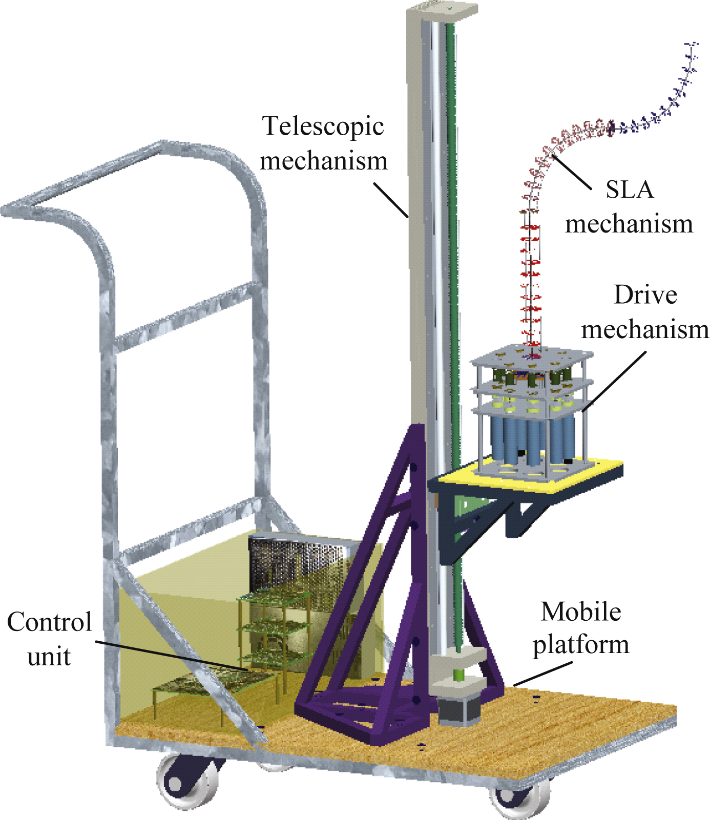
Fig.2
SLA of AFTIR.
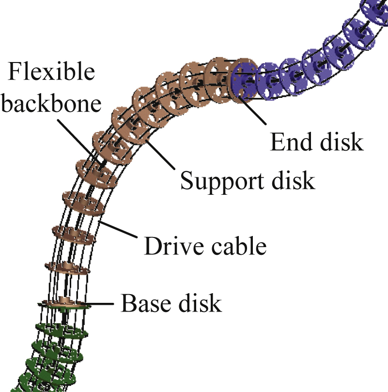
Fig.3
Kinematic model of single JS of SLA.
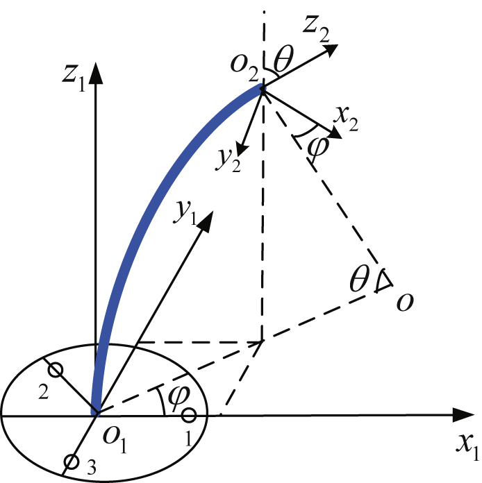
Fig.4
The bending model of JS.
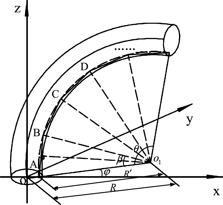
Fig.5
Distribution of threading holes in a disc of JS.
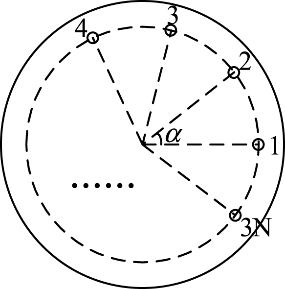
Fig.6
Control block diagram of fuzzy controller.
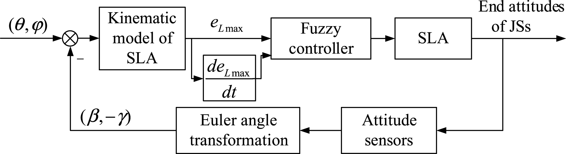
Fig.7
Triangle membership function curve of fuzzy variables.
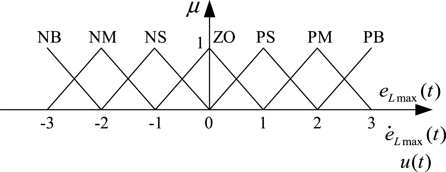
Fig.8
Experimental prototype of a continuum AFTIR.
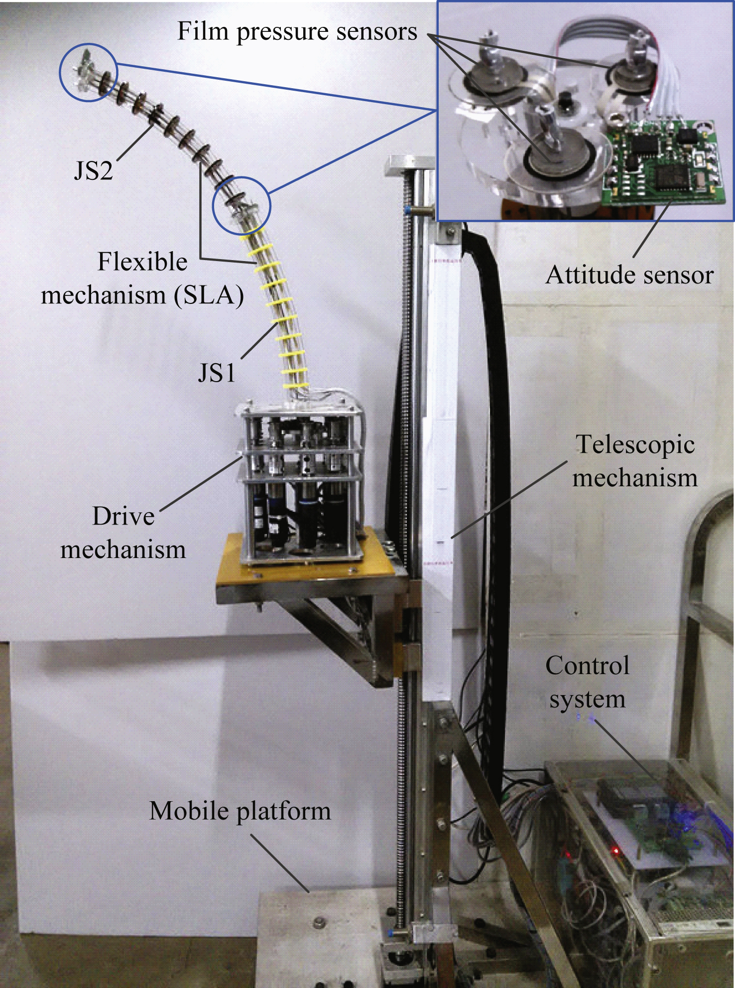
Fig.9
Response curves of SLA.
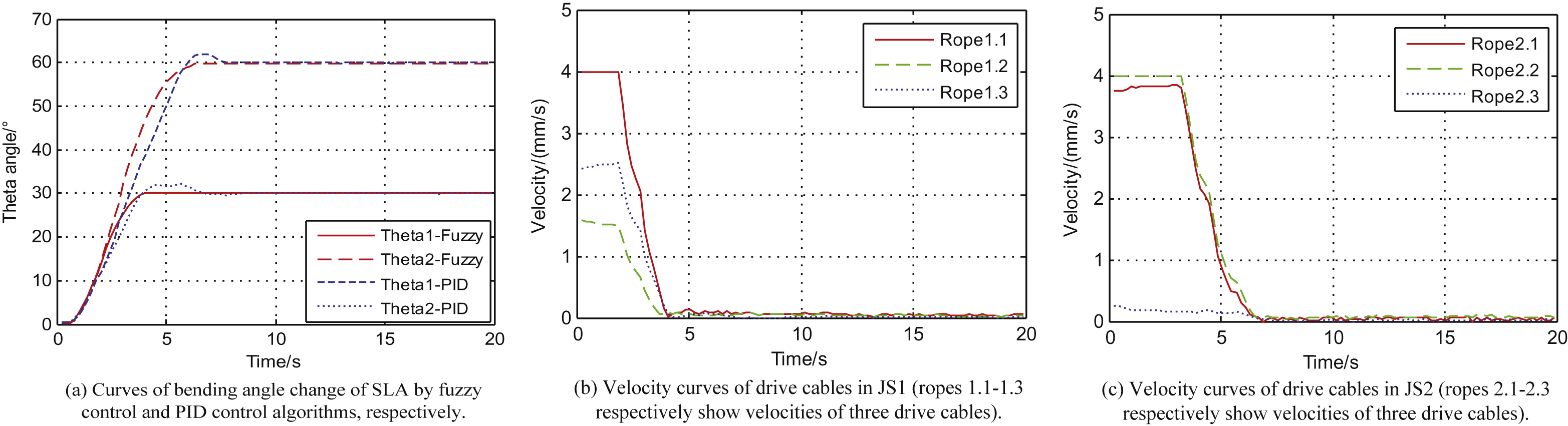
Fig.10
Coplanar bending experiments of two joint segments.
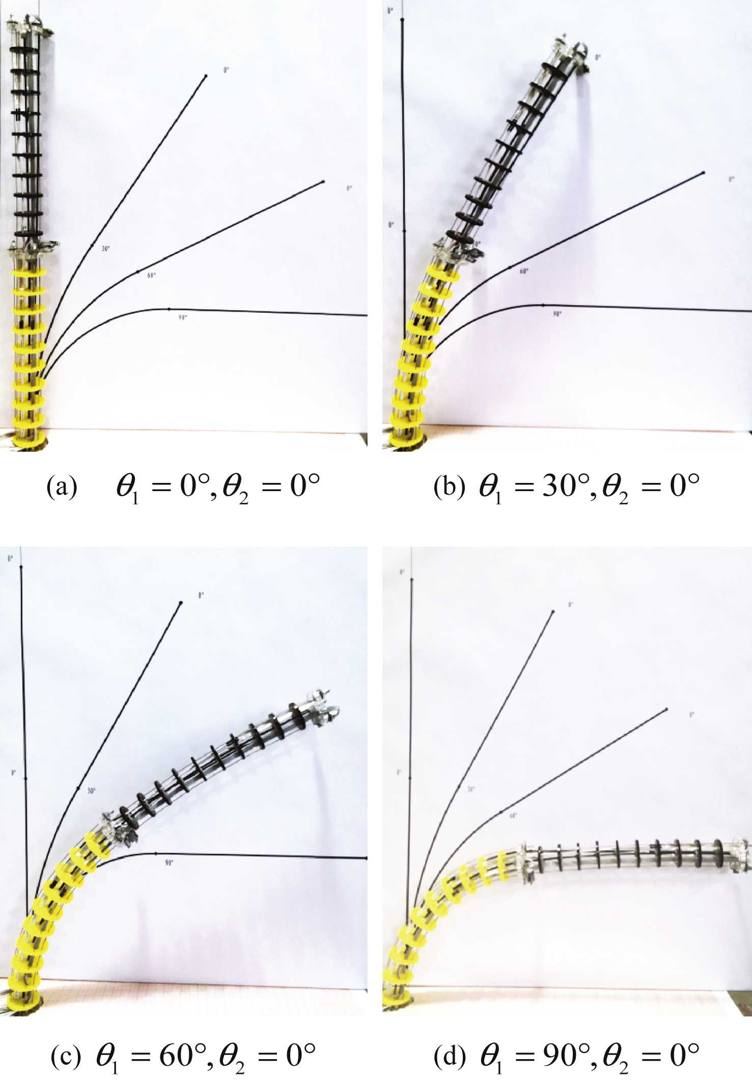
Table 1
Fuzzy control rule base
|
| e Lmax (t) | ||||||
| NB | NM | NS | ZO | PS | PM | PB | |
| NB | PB | PB | PM | PS | NM | NM | NM |
| NM | PB | PB | PM | PS | NM | NS | NM |
| NS | PB | PM | PS | ZO | NS | NM | NM |
| ZO | PM | PS | PS | ZO | NS | NS | NM |
| PS | PM | PM | PS | ZO | NS | NM | NB |
| PM | PM | PM | PM | NS | NM | NB | NB |
| PB | PM | PM | PM | NS | NM | NB | NB |
Table 2
Experiments of bending movement for SLA
| NO. | Set bending angle (°) | Actual angle without correction (°) | Actual angle with correction (°) | |||
| θ 1 | θ 2 | θ 1 | θ 2 | θ 1 | θ 2 | |
| 1 | 0.00 | 0.00 | 0.41 | 1.25 | 0.01 | 0.07 |
| 2 | 30.00 | 0.00 | 28.19 | 34.82 | 29.92 | 30.09 |
| 3 | 60.00 | 0.00 | 56.27 | 69.90 | 59.85 | 60.30 |
| 4 | 90.00 | 0.00 | 84.07 | 104.04 | 89.81 | 90.27 |
| 5 | 30.00 | 30.00 | 29.94 | 62.48 | 30.08 | 59.77 |
| 6 | 30.00 | 60.00 | 31.40 | 87.30 | 30.17 | 89.53 |
| 7 | 30.00 | 90.00 | 32.74 | 113.03 | 30.20 | 119.63 |
Table 3
Performance contrast between fuzzy control and PID control algorithm
| Control | Angle (°) | Rise | Settling | Over |
| algorithm | time (s) | time(s) | shoot (%) | |
| Fuzzy control | θ 1 | 2.24 | 3.46 | 0.70 |
| θ 2 | 3.45 | 5.29 | – | |
| PID control | θ 1 | 2.44 | 3.65 | 7.33 |
| θ 2 | 4.06 | 5.69 | 3.28 |


