
A line planning approach based on harmony search for high-speed rail: From the perspective of service accessibility
Abstract
Service accessibility can be used to describe the travel time of passengers between different nodes, and opportunities to get transportation services in the high-speed railway (HSR) system. Based on the traditional train line planning theory, this paper introduces the transportation service accessibility index, and propose a new nonlinear passenger train line planning model, which aims to maximize the service accessibility, as well as minimize the operational cost of railway company. The model is transformed into a single-objective model, and then we design a harmony search algorithm to solve it. Finally, the model is validated by a numerical example. The results of this model as well as the scenarios of the single-objective models for minimizing operational costs and maximizing service accessibility are compared. From the perspective of service frequency and accessibility of each nodes, we know that the proposed method can balance conflicts between average speed between large nodes and service frequency of small and medium size nodes in high-speed railway network.
1Introduction
Over the past 12 years, China has built the largest high-speed rail network in the world. By the end of 2019, HSR lines operated 35,000 km across the country. In an attempt to optimize the network capacity in order to meet passenger demand, the line planning problem (LLP) is crucial to mitigate the operational issues faced by the rail company. The line plan specifies the routes between origin and destination station, stops and service capacity [12]. The LLP determines the stops, frequencies of train service, as well as train makeup, for services based on passenger demand. Additional information regarding the capacity of each section and station should be utilized efficiently. The LLP operated under the HSR network in China is complicated and difficult to manage in comparison to other countries, such as Germany and Japan, due to its larger size of the network and higher volume of transport demand. The basic objective function of LLP is to minimize the total traveling cost of passenger, maximize the benefits of rail enterprise, and maximize the total passenger that can be transported. While, some shortages are generated from traditional approaches, for example, trains with frequent stations, are organized in this manner to service the demand of intermediate nodes, the total travel time between origins and destinations (ODs) inevitably extends. Due to differences of GDP, population and transport demand among cities along the rail line, service frequencies vary considerably. For example, the average service frequency of small nodes between Beijing and Shanghai HSR is about 6.9 (about two-thirds of the nodes along the line), which means that accessibility of those nodes can be improved. The average travel speed between large-size nodes (such as Beijing, Jinan, Nanjing and Shanghai) is approximately 248 km/h, even though the maximum speed reaches 350 km/h.
In this paper, the service accessibility is presented to evaluate the line plan of rail network, try to get a better line plan for high speed railway by means of balancing the relationship between two conflicting problems, which are improve the travel time among large nodes, and increase service frequencies of middle and small nodes. The paper is organized as follows. Section 2 reviews related line planning literature. Section 3 and Section 4 present a model and algorithm for line planning problem and consider service accessibility. Section 5 is devoted to the evaluation of the numerical experiments. The final section presents major conclusions and gives an outline of future research tasks.
2Literature review
The LPP can be categorized by two typical objective functions of related line planning models: cost-oriented and customer-oriented. Cost-oriented models function to optimize line plan by minimizing operation cost of rail companies and are primarily concerned with the number of trains. Customer-oriented models determine line plan with the objective of optimizing passenger benefits. The model focuses on determining the number of passengers that can be transported and travel cost (such as ticket price and cost of travel time).
Claessens et al. [5] presented integer programming models with cost-oriented objective. Goossen et al. [8, 9] improved upon the model proposed by Claessens, and introduced a branch-and-cut algorithm to solve the LPP. Goerigk et al. [7] further designed a heuristic approach for this problem. Bussieck et al. [1] presented the LPP model to maximize the number of direct travelers. While Scholl [17] remarked that Bussieck’s model may lead to more transfers for travelers and further developed a new model by considering the number of transfers. Guan et al. [10] proposed a new model by minimizing the cost, total passenger and travel time simultaneously, with additional focus on the number of transfers. The researchers follow a similar policy of optimizing train frequencies with pre-given stops. Another policy to solve the LPP, provides an approach that simultaneously optimizes train frequencies and stops. Chang et al. [3] formulated a multi-objective model that minimizes the operation cost, travel time and presents a fuzzy mathematical approach to form a policy that would assist in solving LLP for Taiwan HSR system. Kaspi and Raviv [15] proposed an approach that integrates the line planning, cyclic timetabling, and routing as a new model. Fu et al. [12] presented a hierarchical line planning approach for China HSR network. Su et al. [21] formulated a bilevel optimization model and considered the train operational cost and passenger travel cost in the upper level and passenger assignment in the lower level. Some research focused on algorithm for LPP, such as Column Generation algorithm [19], Simulated Annealing [11].
| Set | |
| G = (S, E) | is the high-speed rail network. |
| Gf = (N, A) | is the service network of line plan. |
| S | is the set of stations/nodes, indexed by s ∈ S. |
| N | is the set of passenger demand nodes, indexed by n ∈ N. |
| E | is the set of sections between stations, indexed by e ∈ E. |
| A | is the set of the service arcs that pass through the corresponding arc of the physical network, indexed by a ∈ A. |
| R | is the set of the potential train service, indexed by r ∈ R. |
| D | is the set of passenger transport demand, indexed by d, d (i, j) ∈ D. |
|
| is the set of arcs that origin from node i. |
|
| is the set of arcs that transport to node i. |
| Parameters | |
| ∂r,i | Boolean parameter, equal to 1 if train service r stops at origin node i, 0 otherwise. |
| ∂r,k | Boolean parameter, equal to 1 if train service r stops at transfer node k, 0 otherwise. |
| ∂r,j | Boolean parameter, equal to 1 if train service r stops at destination node j, 0 otherwise. |
| ϖ | Boolean parameter, equal to 1 if there are transportation services between i and j, and 0 otherwise. |
|
| is the shortest travel time between node i and j. |
| nij | is the number of direct services of type r between i and j. |
| tij | is the shortest direct travel time between i and j. |
| tk | is the average transfer time of node k. |
|
| is the time span of plan horizon. |
| Tij | is the shortest travel time with transfer. |
| lij | is the distance between i and j. |
| v | is the average travel speed of trains. |
| tstop | is the average stop time of trains. |
|
| is the number of stops of service r. |
| m1 | is the operating cost of each train. |
| m2 | is the cost of per kilometer of train operation. |
| m3 | is the cost of train stopping at each station. |
| lr | is the travel distance of service r. |
| xstop,r | means the stop times of intermediate station of line r from i to j. |
| Gj | is the GDP of node j. |
| Pj | is the population of node j. |
| Qd | is the volume of passenger demand d. |
| kr | is the service capacity of service r, that is the makeup and number of seat of trains. |
| Ce | is the passing capacity of section e. |
| ηe | is the correction coefficient of carrying capacity of section e. |
| θra | Boolean parameters, = 1 if service r passing through arc a, and = 0 otherwise. |
| ϑea | Boolean parameters, = 1 arc a belongs to section e. |
| ωrs | Boolean parameters, = 1 if s is the origin station of service r, and = 0 otherwise. |
| ɛr,s | Boolean parameters, = 1 if s is the destination station of service r, and = 0 otherwise. |
| ξr,s | Boolean parameters, = = 1 if service r stops at station s, and = 0 otherwise |
|
| is the capacity for departing trains. |
|
| is the capacity for receiving trains. |
| od | is the origin of demand d. |
| ed | is the destination of demand d. |
| M | is a very large positive number. |
| Decision variables | |
| qda | means the passenger flows that pass through service arc a |
| fr | determines the number of service r during the plan horizon |
There are few researches on the comprehensive optimization of LPP of intercity high-speed railway in network state rather than single line state. Due to the rapid development of urban scale and high-speed railway, the research on the latest development situation of railway network is still insufficient. With the large number of stations and large passenger flow OD, the train operation paths are very large. Therefore, this paper adapts to the actual needs and carries out more in-depth research on the LPP of high-speed railway under the network state.
Accessibility has been a central issue in transport geography and has been broadly used in various fields during the past decades [2, 13, 14]. But there is no research on LPP in HSR based on accessibility. The accessibility can be measured by different indicators that typically measure travel time and quality/quantity. For example, weighted average travel time, daily accessibility, potential accessibility etc, Most of the studies focus on the accessibility of physical transport network. The total travel time of trains is used to calculate such indicators. While this travel time is calculated by minimum on-train time, waiting time for trains (determined by services frequency) at station is unaccounted for. The application of proposed approaches is difficult while measuring the accessibility of service network that presented by line planning of HSR.
3Proposed line planning approach
There are several ways to describe network accessibility, for example, accessibility based on transportation cost, travel time and number of services offered [4, 16, 20]. While, almost all of the research focuses on the accessibility of physical network, in this paper, the SA-HSRLP model based on the service accessibility of high-speed railway line plan is established. This paper takes into consideration the number of services provided and travel time to the destination of a node, in the service network during the plan horizon. The number of services is determined by train frequencies of LPP. Travel time is summation of waiting time at origin station and total travel time to destination. The timespan of planning horizon divided by the train frequencies is the average waiting time and total travel time equal to the travel time between station plus stop time at intermediate stations. From the perspective of HSR network accessibility, different line plans with different train frequency and stops will lead to differentiated service accessibility.
The related notations involved in the SA-HSRLP model are defined as follows:
(1) Multi objective function
Objective function 1: maximization of service accessibility
The high-speed rail network can be set as G = (S, E). The service network of line plan is described as Gf = (N, A). Assume that the stops of line plan are given, we can know the potential train services for each OD. Equation (1) was put forward by Wang et al. [20], which was used to measure the service accessibility of node i. Then the service accessibility F1 of can be formulated as objective function (2) by accumulating all the service accessibility of nodes in one region. The value of
(1)
(2)
The economic and population level of the destination node j is the geometric average of GDP and population
a. the shortest direct travel time between i and j.
Assume that there is only one transfer between any two nodes and if there is more than one node that can be used to transfer during travel time, the one with the shortest transfer time is chosen. Then tij by expression (3) is gotten.
(3)
Where,
(4)
b. the shortest travel time with transfer between i and j:
In order to meet the requirements of fast commuting and ensure the convenience and comfort of passengers, it is assumed that all passengers have at most one transfer during the journey. Considering that there can be multiple transfer points between, the transfer point with the smallest transfer time is taken as the transfer point.
For any transfer node k, the number of direct services to the destination i is:
(5)
After a transfer at station k, the shortest travel time from the start node i to the destination node j is:
(6)
That is, if transfer at node k between node i and j, then node k should have direct service to node j, so
c. the shortest travel time between i and j:
The shortest travel time is the smaller value of direct travel time and travel time with transfer.
(7)
d. convert the shortest travel time to a Boolean value ϖ:
(8)
Objective function 2: minimizing train operation cost:
(9)
We model the LLP with policy of optimizing train frequencies with pre-given stops. The makeup of trains is assumed to be fixed, and passengers always choose the service with shortest travel time with no more than one transfer for the whole trip if there are no direct services. The model of LPP by considering service accessibility is formulated as follows.
(2) constraints of station capacity:
Carrying capacity:
(10)
The actual number of trains passing through the section shall be less than the carrying capacity of the line.
Station capacity of departure:
(11)
The number of departing trains at a station should be less than the departure capacity of the station.
Station capacity of receiving:
(12)
The number of receiving trains at a station should be less than the receiving capacity of the station.
(3) constraints of passenger flow distribution:
Flow conservation:
(13)
In the service network of high-speed railway operation, except for the starting node and the end node, the outflow flow and inflow flow of the intermediate node are equal.
Transportation capacity:
(14)
The number of passengers that are assigned to each arc should not exceed the service capacity of this arc and the service capacity equals to the sum of the number of seats of all trains that pass through each arc.
(4) constraint of integer:
(15)
4Harmony search algorithm
The proposed model is nonlinear, and line planning is a system optimization problem and is extremely complex, especially with the continuous expansion of the current HSR network scale. Some exact solutions are inspirational [24], while there are difficult to apply to this model. Intelligent optimization algorithm is needed to solve the problem. Therefore, according to the characteristics of line planning problem, it is of great practical significance to study and select the appropriate optimization algorithm, so as to quickly obtain satisfactory train operation scheme. Compared with ILOG, Gurobi and other optimization software, although heuristic algorithm cannot guarantee the optimality of the solution, and even cannot explain its approximation to the optimal solution in most cases, it can find the feasible solution in the acceptable cost and time range. This is consistent with the requirements of train operation plan preparation: to obtain a feasible plan within an acceptable time.
According to the characteristics of the model, this paper uses harmony search algorithm (HS) to solve the model. Compared with traditional heuristic algorithms such as genetic algorithm (GA), ant colony algorithm and simulated annealing algorithm, harmony search algorithm has the characteristics of easy understanding, simple steps, novel solution construction, easy programming and calculation, and less adjustment parameters.
Compared with the traditional GA, the initial solution generation of HS algorithm is random, and both of them have the evaluation mechanism of fitness function. HS algorithm has crossover and mutation operations similar to GA, so it has most of the advantages of GA. At the same time, because the HS algorithm produces a new solution clearly, only one new solution is generated in each iteration, so the complexity is low. In view of the advantages of HS algorithm, this paper intends to use HS algorithm to solve the line planning problem.
The model proposed in the previous section is a multi-objective nonlinear integer programming model. To tackle it, we first transform this model into a single-objective one and then design an algorithm based on Harmony Search [6, 18] to resolve it.
The solution can be presented as (16, where fr is a positive integer, which means that the frequency of pre-given service is r. We generate initial solution by getting a number randomly in the interval [0, Ce] for each r. If the size of Harmony Memory (HM) set to be HMS, then get the HM as shown as (17).
(16)
(17)
During the iteration, new solutions can be generated as follows. First, get a random number from [0,1], note as rand, compare rand with HMCR (probability to choose a solution from HM). If rand < HMCR, then select a solution from HM randomly. Disturb this selected solution with probability of PAR, and disturbance strategies include, reduction of one time of service of any r. If its frequency is more than 1, or add one time of service of any r if its frequency is no more than Ce – 1. If rand≥HMCR, generate a new solution as the way to get the initial solution.
For multi-objective optimization problems, Nyoman [22] introduced the scalarization method to convert the problem to a single-objective one. As Liu [23] did, the multi-objective function is converted as (18).
(18)
For each solution that in HM or new generated, we need to assign passenger flow to those services. We first search the K-shortest path for each OD based on the total travel time. We assume the passenger chooses the direct trains with priority and select the service with shortest travel time among those direct trains. If there are no direct trains, passengers can choose the transfer service with the shortest travel time. We can assign the passenger flow to the shortest path (service) based on all-or-nothing policy. Finally, the penalty function is used to deal with the infeasible solution if the passenger flow cannot be assigned to the service network.
The procedure of this algorithm then can be presented as follows;
Step 1: parameter initialization.
Step 2: generation of the initial HM and calculation of the values of objective function of solution in HM.
Step 3: generation of a new solution.
Step 4: compare the value of the new solution and that’s the solution in HM, and then update the HM.
Step 5: end for pre-given number of iteration steps, or back to Step 3.
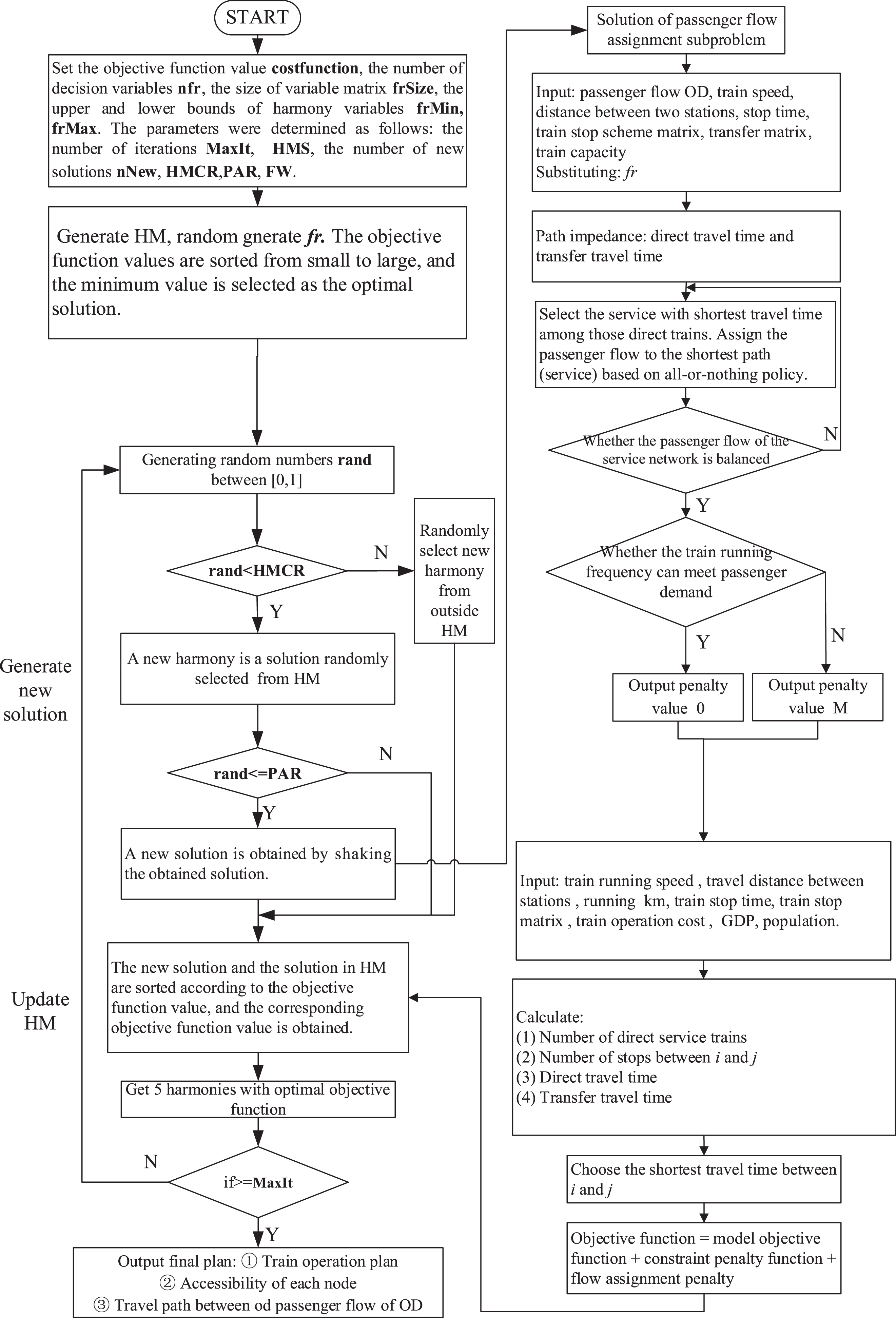
The complete algorithm flow is shown in Fig. 1.
Fig. 1
Algorithm flow.
5Numerical experiments
We now present the numerical experiment of the above line planning approach that consider service accessibility. The HSR network and pre-given train services are shown as under Fig. 2. The section mileage, GDP and population of each node, the passenger demands are present in Tables 1 to 3.
Fig. 2
HSR network and pre-given line plan.
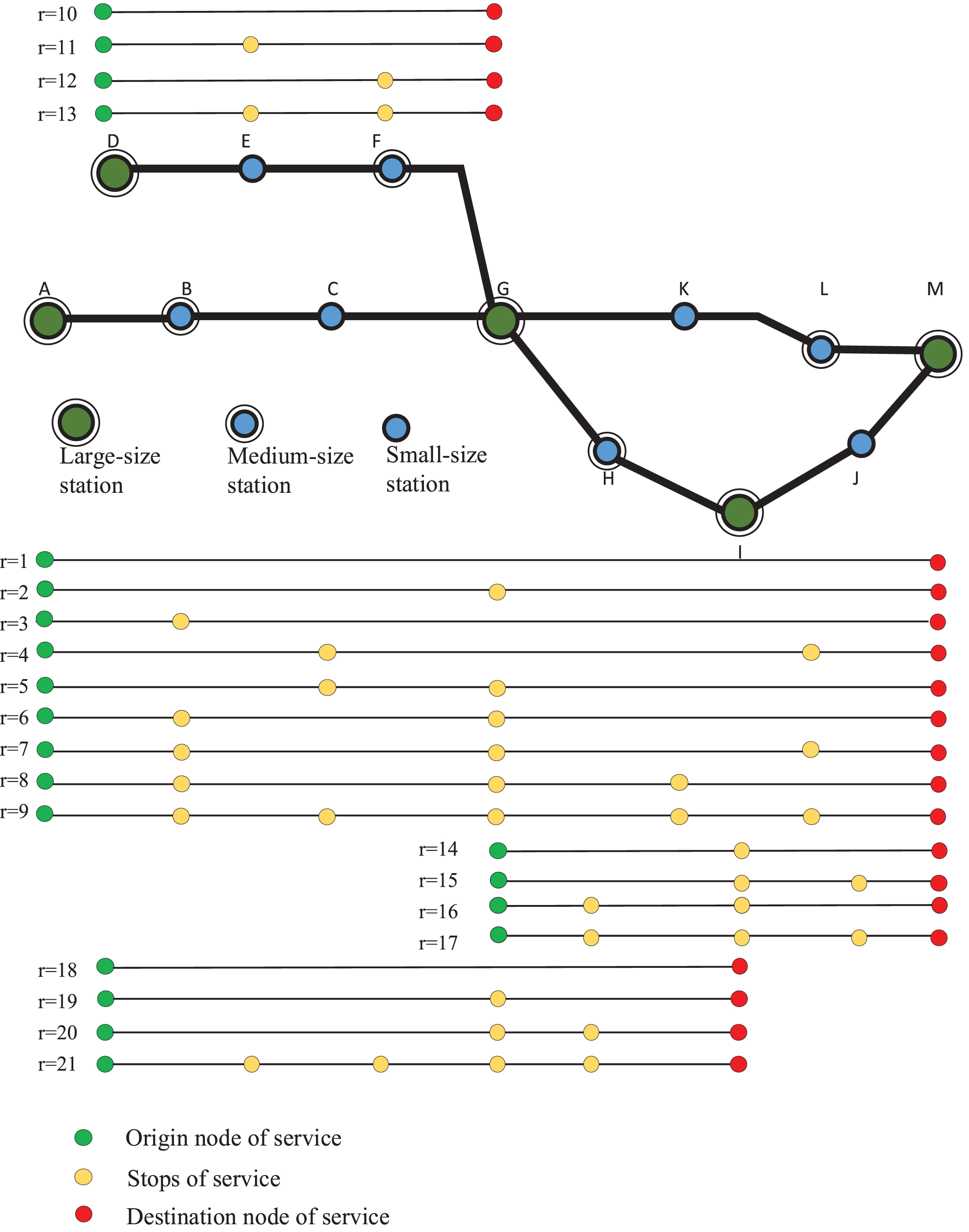
Table 1
Mileage of each section
| No. | Sections | Length(km) | No. | Sections | Length(km) |
| 1 | (A, B) | 47.3 | 8 | (E, F) | 45.2 |
| 2 | (B, C) | 47.5 | 9 | (F, G) | 49.1 |
| 3 | (C, G) | 46.5 | 10 | (G, H) | 47.3 |
| 4 | (G, K) | 48.2 | 11 | (H, I) | 45.4 |
| 5 | (K, L) | 45.7 | 12 | (I, J) | 47.7 |
| 6 | (L, M) | 48.7 | 13 | (J, M) | 47.4 |
| 7 | (D, E) | 47.8 |
Table 2
GDP and population of each node
| Node No. | GDP (100 million) | Population (10 thousand) | Node No. | GDP (100 million) | Population (10 thousand) |
| A | 28000 | 21700 | H | 623 | 2670 |
| B | 277 | 760 | I | 10002 | 18520 |
| C | 145 | 570 | J | 149 | 570 |
| D | 5465 | 11790 | K | 102 | 480 |
| E | 87 | 400 | L | 348 | 1490 |
| F | 324 | 1230 | M | 6460 | 10780 |
| G | 1119 | 30000 |
Table 3
Passenger flow of each OD on the down bound of the HSR network
| O/D | A | B | C | D | E | F | G | H | I | J | K | L | M |
| A | 0 | 634 | 192 | 0 | 0 | 0 | 1534 | 253 | 335 | 11 | 122 | 425 | 2753 |
| B | 0 | 53 | 0 | 0 | 0 | 513 | 124 | 62 | 5 | 103 | 364 | 445 | |
| C | 0 | 0 | 0 | 0 | 117 | 18 | 29 | 4 | 36 | 235 | 326 | ||
| D | 0 | 43 | 132 | 645 | 426 | 1324 | 123 | 24 | 33 | 1314 | |||
| E | 0 | 123 | 575 | 262 | 734 | 5 | 53 | 6 | 132 | ||||
| F | 353 | 232 | 642 | 17 | 14 | 135 | 231 | ||||||
| G | 0 | 474 | 637 | 24 | 23 | 76 | 856 | ||||||
| H | 0 | 134 | 58 | 0 | 0 | 161 | |||||||
| I | 0 | 88 | 0 | 0 | 656 | ||||||||
| J | 0 | 0 | 0 | 25 | |||||||||
| K | 0 | 67 | 236 |
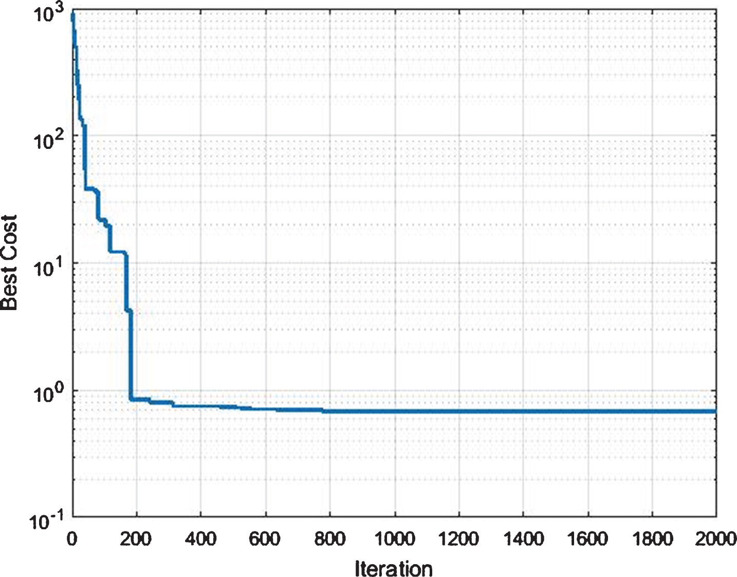
This algorithm is written in Matlab and run on an Intel i3 with 4 G Ram. After several time tests, we set the parameters of this algorithm as: HMS = 35, HMCR = 0.9, PAR = 0.1, the maximum iterations are 2000. After near 800 iterations in 180 seconds, the final solution as shown in Fig. 3, 13 services are selected from pre-given 21 potential choices, and the total number of trains are 23. The iterative convergence is shown in Fig. 4.
Fig. 3
Final solution of this multi-objective function model.
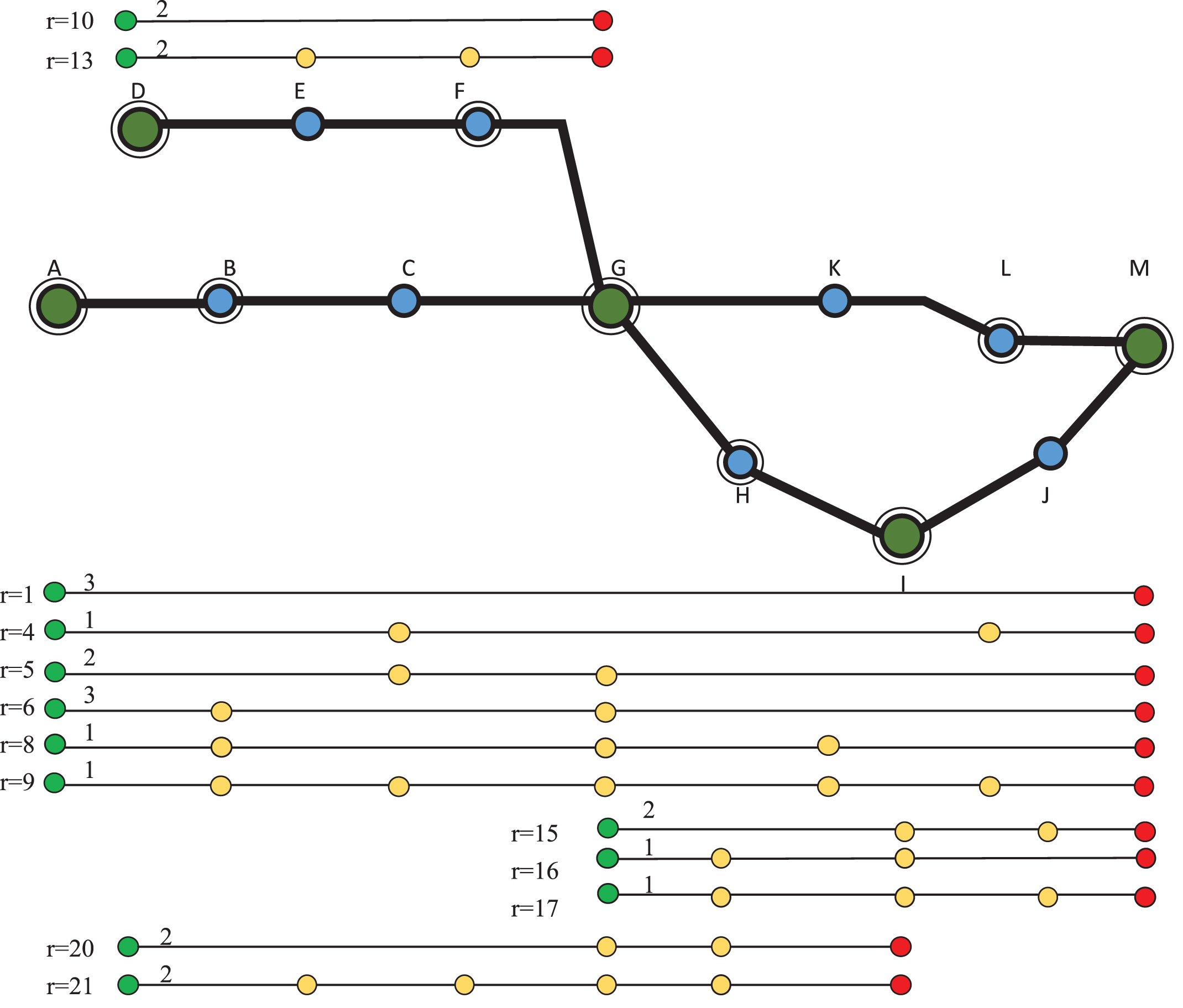
Fig. 4
Iterative convergence of algorithm.
Results analysis of the numerical experiments.
(1) Number of trains under different objective function.
The waiting time at the origin station can be reduced by adding more trains for service. While, from the perspective of operator, more trains under operation means larger cost. The experiment tested and compared the solution of modes with multi-objective function (M), with the single objective function of minimizing operation cost (SC) and the best service accessibility (SA). The results are shown in Table 4. The number of trains in the three scenarios are 23, 19 and 28 respectively. In order to minimize operation cost, the rail company can organize trains that have more stops, which will compromise the level of service of HSR. So we add the cost of each stop in the objective function, in order to adjust the number of trains with poor level of service, such as the train that stop at all of the intermediate stations.
Table 4
Result comparison among different objective function
| Scenarios | r | 1 | 2 | 3 | 4 | 5 | 6 | 7 | 8 | 9 | 10 | 11 |
| M | fr | 3 | 0 | 0 | 1 | 2 | 3 | 0 | 1 | 1 | 2 | 0 |
| SA | fr | 0 | 0 | 0 | 4 | 0 | 4 | 0 | 0 | 4 | 0 | 0 |
| SC | fr | 3 | 0 | 0 | 1 | 0 | 3 | 1 | 0 | 1 | 0 | 1 |
| r | 12 | 13 | 14 | 15 | 16 | 17 | 18 | 19 | 20 | 21 | ||
| M | fr | 0 | 2 | 0 | 2 | 1 | 1 | 0 | 0 | 2 | 2 | |
| SA | fr | 0 | 0 | 3 | 0 | 0 | 3 | 4 | 0 | 0 | 6 | |
| SC | fr | 0 | 0 | 0 | 1 | 0 | 2 | 0 | 3 | 2 | 1 |
Under scenario SA, train services of 9, 17 and 21 have been planed 4, 3 and 6 train during the plan horizon. For the scenario of SC, the number are 1, 2 and 1, respectively. So, we know that, more trains with more stops can improve the service accessibility of nodes and network. While, the transport demand of large nodes in the network will spend more time on trains. Under scenario M, more trains that service large nodes and have small number of stop at intermediate nodes have been organized. For example, we planned train service r = 1 and r = 10, which are direct trains just service large node. And trains service r = 5 and r = 15 that origin and terminate at large nodes and stops at a small number of the other node are planned simultaneously. The travel time for the passenger from large nodes and service opportunity for passenger from intermediate and small nodes can be well balanced.
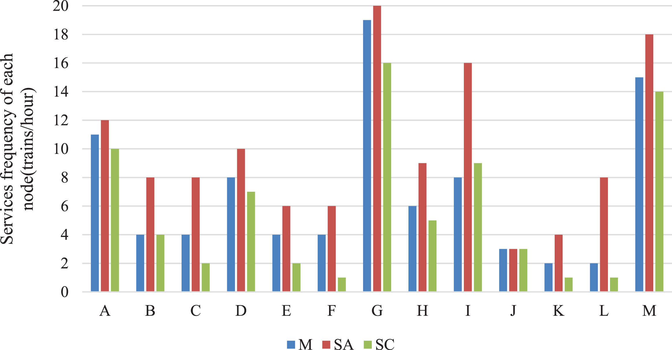
(2) Service frequencies of nodes under different objective function.
The result is shown in Fig. 5. Compare to the scenario SC, the service frequencies of nodes A, C, D, E, F, G, H, K, L and M are increased in scenario M. Some of the medium-size node, such as C, E and F, the service frequencies increased 2 trains, 2 trains and 3 trains per hour.
Fig. 5
Service frequencies of nodes.
(3) Service accessibility of nodes and network.
The accessibility of network of scenario M, SC and SA are 9.35, 10.81 and 7.34 respectively. The service accessibility of nodes is shown in Table 5. We know that service accessibility of nodes under scenario M is better than that of scenario SC, as none of the nodes service accessibility of scenario SC is better than scenario M, 71.4% of those nodes are medium and small nodes.
Table 5
Service accessibility of nodes
| Scenarios | A | B | C | D | E | F | G | H | I | J | K | L |
| M | 1.06 | 0.96 | 0.88 | 0.99 | 0.90 | 0.69 | 0.63 | 0.85 | 0.69 | 0.47 | 0.76 | 0.47 |
| SA | 0.97 | 0.83 | 0.68 | 0.79 | 0.78 | 0.56 | 0.56 | 0.47 | 0.56 | 0.33 | 0.47 | 0.33 |
| SC | 1.08 | 0.96 | 0.80 | 1.19 | 1.41 | 0.84 | 0.63 | 0.81 | 0.57 | 0.63 | 0.80 | 1.08 |
6Conclusions
This paper introduces service accessibility into tradition line planning problem of HSR. The service accessibility is determined by the number of services, trip time to the destination of a node and the service network during the planned horizon. From the perspective of line plan, service accessibility depends on the trains frequencies and stops. The study proposed a multi-objective nonlinear model for HSR line planning problem which aims to balance the travel time between large-size nodes and the service accessibility of medium and small size nodes in HSR network. A heuristic based on Harmony Search is designed after transformation of the model into a single-objective function one. The results of numerical experiment show that proposed approach can improve service accessibility of the whole network and most of the medium and small size nodes, as compared to the model with single objective function of minimizing the operation cost.
In practice, there may be more than one transfer when the transportation of large HSR network as China is considered. The study intends to further enhance its model by contemplating a transport system through more than one transfer when no direct trains are available. In addition, further case studies with real world data will be utilized to test the model and algorithm and will be discussed further.
Acknowledgments
This research was jointly supported by National Key R&D Program of China (2018YFB1201402), and National Natural Science Foundation of China (No. 71701014).
References
[1] | Bussieck M. , Optimal Lines in Public Rail Transport, Ph.D. Thesis, TU Braunschweig, Germany. (1998). |
[2] | Cao J. , Liu X.C. , Wang Y. and Li Q. , Accessibility impacts of China’s high-speed rail network, Journal of Transport Geography 28: ((2013) ), 12–21. |
[3] | Chang Y.H. , Yeh C.H. and Shen C.C. , A multi-objective model for passenger train services planning: application to Taiwan’s high-speed rail line, Transportation Research Part B 34: ((2000) ), 91–106. |
[4] | Chen Z. and Haynes K.E. , Impact of high-speed rail on regional economic disparity in China, Journal of Transport Geography 65: ((2017) ), 80–91. |
[5] | Claessens M.T. , van Dijk N.M. and Zwaneveld P.J. , Cost optimal allocation of passenger lines, European Journal of Operational Research 110: ((1998) ), 474–489. |
[6] | Geem Z.W. , Kim J.H. and Loganathan G.V. , A New Heuristic Optimization Algorithm: Harmony Search, Simulation 76: (2) ((2001) ), 60–68. |
[7] | Goerigk M. , Schachtebeck M. and Schöbel A. , Evaluating line concepts using travel times and robustness, Public Transport 5: ((2013) ), 267–284. |
[8] | Goossens J. , van Hoesel S. and Kroon L. , A branch-and-cut approach for solving railway line planning problems, Transport Science 38: ((2004) ), 379–393. |
[9] | Goossens J. , van Hoesel S. and Kroon L. , On solving multi-type railway line planning problems, European Journal of Operational Research 168: ((2006) ), 403–424. |
[10] | Guan J.F. , Yang H. and Wirasinghe S.C. , Simultaneous optimization of transit line configuration and passenger line assignment, Transportation Research Part B 40: ((2006) ), 885–902. |
[11] | Su H.Y. , Shi F. , Deng L.B. , et al., Time-dependent Demand Oriented Line Planning Optimization for the High-speed Railway, Journal of Transportation Systems Engineering and Information Technology 16: (5) ((2016) ), 116–116,135. |
[12] | Fu H.L. , Nie L. , Meng L.Y. , et al., A hierarchical line planning approach for a large-scale high-speed rail network: The China case, Transportation Research Part A 75: ((2015) ), 61–83. |
[13] | Wang L.H. , Liu Y.X. , Sun C. and Liu Y.H. , Accessibility impact of the present and future high-speed rail network: A case study of Jiangsu Province, China, Journal of Transport Geography 54: ((2016) ), 161–172. |
[14] | Jiao J.J. , Wang J. , Jin F.J. and Dunford M. , Impacts on accessibility of China’s present and future HSR network, Journal of Transport Geography 40: ((2014) ), 123–132. |
[15] | Kaspi M. and Raviv T. , Service-oriented line planning and timetabling for passenger trains, Transportation Science 47: (3) ((2013) ), 295–311. |
[16] | Moyano A. , Martinez H. and Coronado J.M. , From network to services: A comparative accessibility analysis of the Spanish high-speed rail system, Transport Policy 63: ((2018) ), 51–60. |
[17] | Scholl S. , Customer-oriented Line Planning, Ph.D. Thesis, University of Kaiserslautern, Germany. (2005). |
[18] | Shahraki A. and Ebrahimi S.B. , A new approach for forecasting enrollments using harmony search algorithm, Journal of Intelligent and Fuzzy Systems 28: (1) ((2015) ), 279–290. |
[19] | Pu S. , Lv H.X. , Chen D.J. , et al., High Speed Railway Passenger Train Line Planning Optimization Based on Improved Column Generation Algorithm, Journal of the China Railway Society 36: (9) ((2015) ), 1–7. |
[20] | Wang L. , Liu Y. , Sun C. , et al., Accessibility impact of the present and future high-speed rail network: A case study of Jiangsu Province, China, Journal of Transport Geography 54: ((2016) ), 161–172. |
[21] | Su H.Y. , Tao W.C. and Hu X.L. , A Line Planning Approach for High-Speed Rail Networks with Time-Dependent Demand and Capacity Constraints, Mathematical Problems in Engineering 2019: Article ID 7509586. ((2019) ). |
[22] | Nyoman G. and Qingsong A. , A review of multi-objective optimization: methods and its applications, Cogent Engineering. (2018). |
[23] | Liu X.C. , Research on Product Design and Collection Distribution System Organization in Railway Freight Corridor Based on improvement of Transport Capacity, Beijing Jiaotong University, Beijing, (2015), 102–103. |
[24] | Ali M. and Ma W. , New Exact Solutions of Nonlinear (3+1)-Dimensional Boiti-Leon-Manna-Pempinelli Equation, Advances in Mathematical Physics (2019), 1–7. |


