
Boris Kovalerchuk, Visual Knowledge Discovery and Machine Learning Springer, Cham, Switzerland, 2018
What we humans want. We want to learn the current state of the world, we want to predict the future state of the world, and we want to find out what decisions and actions we need to undertake to make this future state the most beneficial to us.
For all these tasks, we need to know the dependence between different quantities. How can we do it? Let us start with how we learn the current state of the world. To know the current state of the world means to know the values of all the quantities that describe this state. Some of these quantities we can simply measure: e.g., we can measure the temperature at any given location on Earth. Other quantities are not so easy to measure directly – e.g., there is no way to directly measure the temperature on the surface of the Sun, or, more generally, on a surface of a star.
To learn the values of such difficult-to-measure quantities y, we need to find some easier-to-measure quantities x1, …, xn that are related to the desired quantity y by a known dependence y = f (x1, …, xk). Then, we can measure these auxiliary quantities xi, and use the results xi of these measurements and the known dependence between xi and y to estimate the value of y.
Similarly, to predict the future state of the world means to predict the values of all the quantities y that describe this future state. To predict each of these value y based on the current state of the world – i.e., based on the current values x1, …, xn of different quantities, we need to know how y depends on xi, i.e., we need to know the dependence y = f (x1, …, xn) between the current and the future values of different quantities.
To find the decisions or actions which will lead to most beneficial future, we need to find out how the quality y of the future state will depend on the parameters xi describing our actions.
In all these cases, we need to know the dependence y = f (x1, …, xn) between different quantities. In some cases, we already know this dependence, but in many other cases, we need to determine this dependence based on the known results of measurements and observations. Usually, we have some cases k = 1, …, K in which we know the values
Need to supplement machine learning with visualization. In general, finding the dependence based on examples is the main objective of machine learning. In many cases, machine learning techniques have indeed successfully found the desired dependence. However, in spite of all the successes, machine learning is not (yet) a panacea. There are many practical situations where its methods do not succeed.
So, a natural idea is to use our own abilities to help machine learning algorithms – or even to find the dependencies ourselves, without the help of these algorithms. How can we do it? If we simply look at the numbers that form the data, we will most probably not come up with any ideas. A natural idea is to plot – i.e., visualize – the data points, this often helps.
For example, if we are interested in the dependence of y on only one variables x1 (i.e., if n = 1), then we can plot the observed pairs (x1, y) and see if the resulting points form one of the known dependencies. Often, to see this dependence, we need to re-scale the data. We need to re-scale, if the dependence is too close to a constant. After that, we sometimes immediately see that the resulting dependence is close to a linear or to a quadratic dependence. Sometimes, we need to apply a non-linear re-scaling: e.g., the way to recognize power laws y = c · xa is to use the fact that in this case, ln(y) = a · ln(x) + ln(c) and thus, in the log-log scale, we will have a linear dependence between re-scaled variables
But how can we visualize multi-D data? In most practical problems, the number n is large. Can can we visualize such a dependence?
Sometimes, the set of all the points
One of the possibilities is to use Parallel Coordinates: to represent (n + 1)-dimensional data, we draw n vertical lines corresponding to n + 1 variables and represent each point
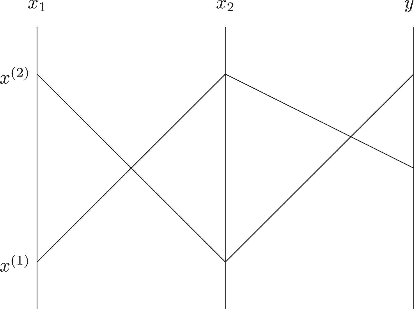
Similarly to the 2-D case, we can appropriately re-scale each of the values xi and y. We can place lines at some angle to each other. We can also use the curved lines to represent each of the values xi and y, and we can use the curved lines to connect the corresponding points.
In some cases, variables can be naturally divided into pairs. In this case, each pair can be represented as a point on the plane, and points corresponding to different pairs can be connected, e.g., by straight lines. For example, if x1 is naturally connected with x2, and x3 is naturally connected with y, then we can represent a multi-D point (x1, x2, x3, y) by drawing two points (x1, x2) and (x3, y) and connecting them by a straight line segment.
All such representations are called General Lines Coordinates (GLC). Studying such representation is the main topic of the book.
What the book does. The book describes different GLCs, studies their properties, provides algorithms for generating GLCs and for detecting basic dependencies based on such representations. It describes the results of user-based experiments which show which GLCs are better and when. It also shows how to combine these techniques with machine learning.
And it lists many applications to practical problems, where the corresponding visual analysis indeed helps. These example range from the study of the Challenger disaster to the analysis of World hunger data, health monitoring and computer-aided medical diagnostics, image processing, text classification, and prediction of the currency exchange rate.
Who should read this book. First, practitioners. The author’s examples show that the corresponding visualization can help in various applications. Clearly, this is something to try when you encounter new multi-dimensional data. Second, researchers. The book has many interesting results, but it also lists many open problems. In the reviewer’s opinion, one of the main open problems is: how to select the best GLC representation? There are many of them, each of them is known to be useful in some problems, it would be nice to have a general guidance of when each of them should be used.
Finally, students (and their teachers). This is a well-written book, with plenty of material that will help students in their future work.


