
Application of semantic location awareness computing based on data mining in COVID-19 prevention and control system
Abstract
Because of the global spread of COVID-19 in 2020, the analysis of activities and travel behavior of urban residents is the key for the prevention and control of epidemic situation. Based on this, the research on track data mining and semantic location perception is conducted. The analysis of travel behavior characteristics of urban residents is helpful to carry out epidemic prevention activities scientifically. However, the traditional manual survey and statistical analysis cannot meet the needs of the rapid development of urbanization. On the other hand, with the application and development of information technology such as communication, location and storage, a large number of mobile trajectory data of urban residents can be collected and stored. These trajectory data contain rich spatiotemporal semantic information. Through mining and analysis, a lot of valuable travel information can be get and then the daily behavior of individual users and the spatial distribution characteristics of group users’ movement can be found. The results can effectively serve the current epidemic prevention work and can be applied to the infection tracking in the process of epidemic prevention.
1Introduction
The activity and travel behavior of urban residents is an important part of urban activity mobile system. The analysis of the characteristics of urban residents’ travel behavior is conducive to the scientific urban planning and traffic management, especially during the period of COVID-19. The prevention and control mechanism is the most important for the monitoring of infected people and their close contacts. However, the traditional manual survey and statistical analysis cannot meet the needs of the rapid development of urbanization. On the other hand, with the application and development of information technology such as communication, location and storage, a large number of mobile trajectory data of urban residents can be collected and stored, which contains rich spatiotemporal semantic information. Through mining and analysis, a lot of valuable travel information can be obtained, and then the daily behavior rules of individual users and group user mobility can be found. The results can effectively serve the fields of intelligent transportation and urban planning [1–5].
In the past few years, some service applications still stay in the simple location-based service applications such as recommending the stores near the user’s surroundings according to the user’s current GPS fixed point, without further digging the track information before the user to provide more convenient and intelligent services for the user. At present, the research of trajectory mining is also in the stage of theoretical research based on some research data, which is limited to the overall trajectory data information environment.
This paper is devoted to the research of spatiotemporal trajectory data mining method and its application in the analysis of urban residents’ travel behavior pattern [4–10]. Firstly, the spatiotemporal trajectory data model is constructed, and a method of outlier detection based on the public segment subsequence is proposed, and the abnormal route is analyzed by combining with the personal travel trajectory data of city A; secondly, the trajectory clustering method based on the multi feature similarity measurement model is designed and verified by the analysis of the residents’ routine travel routes; secondly, the information entropy and multi feature are proposed Finally, based on the taxi track data set of city a, this paper analyzes the travel spatial characteristics of urban residents from multiple perspectives, such as hot spot distribution and mobile mode, and proposes a hot spot location mining method based on neighborhood association quality clustering, and through the analysis of residents’ travel commuting and outgoing The detection of hot spot area of car rental is verified by an example [11–13].
2System design and implementation
Road network refers to the road system composed of various roads in a certain area and interwoven into a network distribution. The road network in the urban area is called urban road network. The road network can be represented as a directed graph G = (V, E) , V = {n1, n2, ⋯ , nVN} representing the set formed by the end points of VN road sections in the road network space, E = {e1, e2, ⋯ , eEN} representing the set formed by the EN road sections between the end points of road sections, each directed edge is recorded as
This experiment is based on the implementation of a city vector electronic map data on ArcGIS platform. Figure 1 shows part of the road network in the central city of Beijing vector electronic map. Among them, the basic data of road network is road section, and a road is a collection of several road sections.
Fig. 1
A road network data of downtown area.
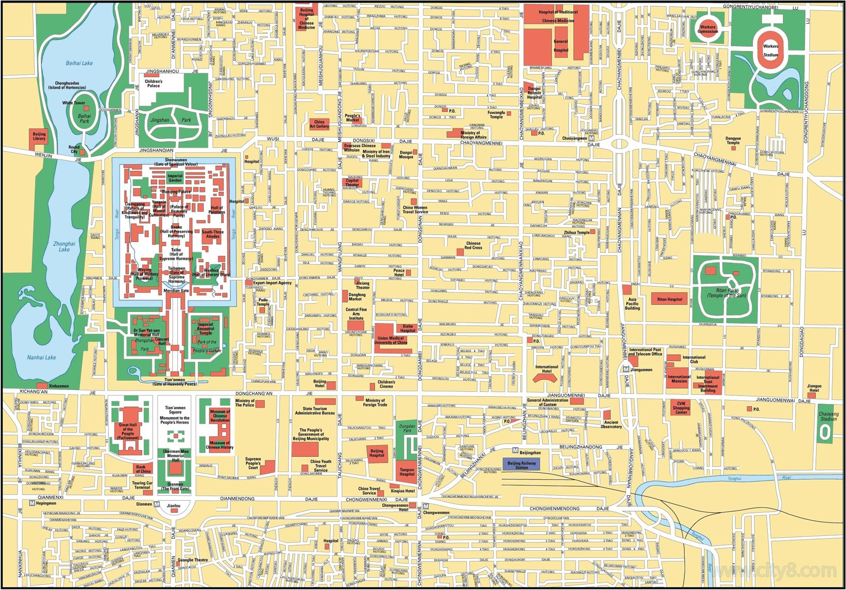
The map shows the end points of urban expressway and Township Village Road. The attribute data of the section highlighted in blue in the middle is shown in Table 1, where id is the number of the selected section, (SX, SY) and (ex, ey) represent the longitude and latitude coordinates of the starting point and the ending point of the section respectively.
Table 1
Some attribute data of the selected section
| ID | MAPID | NAME | SX | SY | EX | EY |
| 404796 | 595679 | Second ring | 119.0637 | 93.4396 | 118.0808 | 37.2200 |
Based on the above information, the track map matching algorithm is constructed, and the map matching algorithm is divided into two stages. They are road network division and extraction of road segment information in grid, aiming at road network matching of each track.
The first stage: road network division and road segment information extraction in grid. There are two stages;
STAGE 1: Grid the road network data.
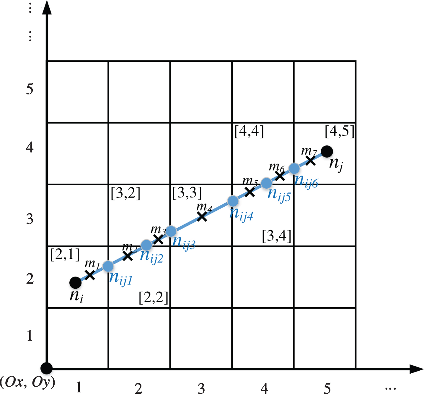
Step 1: Grid the road network data. Take the coordinate point of the lower left corner of the road network map as the origin of the road network grid coordinate system (ox, oy), set the coordinate point of the upper right corner of the road network map to (Mx, My), and take gridlat and gridlong as the unit degrees respectively Grid the latitude and longitude directions. The road network map is divided into [(My - oy)/gridlat] × [(Mx - ox)/gridlong] grid, where the number of each two-dimensional grid is jointly represented by the sequence number of the row and column in which it is located. For example, the grid number with row number of 2 and column number of 1 is [2,1]. For any location point (xk, yk) in the road network, its grid number is recorded as [Gki, Gkj], which can be calculated as follows:
(1)
(2)
Step 2: Get the road information in each grid of the road network.
After the road network map is divided into a series of two-dimensional grids, the grid sequence of each road section and the road section information contained in each grid can be obtained.
In order to obtain the information of each road segment in each grid of the road network, we can first calculate the grid that each road segment passes through, and then carry out the road segment statistics for each grid. As shown in Fig. 2, <ni, nj> is a road section in the road network. The grid it passes through includes [2,1], [2,2], [3,2], [3,3], [3,4], [4,4], [4,5]. Take this section as an example to describe the specific method of obtaining the grid of the section in this paper:
(1) Calculate the intersection point nij1, nij2, ⋯ , nij6 of section <ni, nj> and all grid lines, and divide the section into 7 sub sections <n1, nij1> , < nij1, nij2 > , ⋯ , < nij6, nj >;
(2) Calculate the center point m1, m2, ⋯ m7 of each sub section, where
and so on.(3)
(3) According to formula (1) and formula (2), the grid numbers of starting and ending point ni, nj and central point m1, m2, ⋯ , m7 of sub section are calculated respectively, and all grid information of section <ni, nj> is obtained.
Fig. 2
A road network data of downtown area.
After extracting the grid information of all road sections in the road network, we can count and record the road section number contained in each grid, so as to obtain the road section information, and record the road section information in each grid of the road network in the gridsinfo table.
STAGE 2: Road network matching for each track.
Set the input as an original track and the output as a new track after map matching. For each location point in the original track, find the grid where it is and all the sections in the adjacent grid, and calculate the projection point of the location point on the most matching section as its map matching point. Specific steps:
Step 1: Calculate the grid number B of the first location point a.
Step 2: Based on the information in gridsinfo, extract all sections of [G1i, G1j] and its adjacent grid, calculate the distance between (x1, y1) and its projection point on each section, and find the section projection point closest to (x1, y1) as the map matching point.
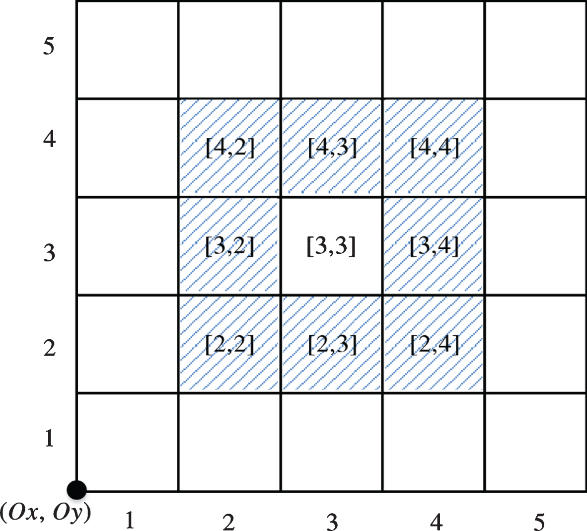
The adjacent grid of grid [G1i, G1j] refers to eight adjacent grids, which are
For example, the nearest neighbor grid of grid [3,3] refers to eight grids [2,2], [3,2], [4,2], [2,3], [4,3], [2,4], [3,4], [4,4], as shown in Fig. 3.
Fig. 3
Example of nearest neighbor grid.
Step 3: Starting from the second location point, calculate the grid number of each location point in turn, extract all sections of the grid and its adjacent grid, get the set of projection points of the location point on each section, and calculate the previous map matching point to the points based on the combined section table. The shortest path length of each projection point in propoints is taken as the map matching point of the current location point.
Step 4: Repeat step 3 until all position points in the track are processed.
3Detailed design scheme of the system
3.1Database design
The Table 2–8 shows the parameter setting process.
Table 2
User Table G-user
| Column name | data type | |
| Un | Int | Primary key |
| Uname | Nchar (20) | |
| Uphone | Nchar (20) |
Table 3
Track route Table G-line
| Column name | data type | |
| In | Int | Primary key |
| Gstar | Int | |
| Gend | Int | |
| Un | Int | Foreign key (G-user) |
Table 4
Track data sheet G-data
| Column name | data type | |
| Dn | Int | Primary key |
| Time | Int | |
| x | Int | |
| y | Int |
Table 5
Address Table
| Column name | data type | |
| a-id | int | Primary key |
| a-name | ncbar | |
| a-count | int |
Table 6
Location data sheet address
| Column name | data type | |
| a-d-id | int | Primary key |
| a-d-x | int | |
| a-d-y | int |
Table 7
Relation Table
| Column name | data type | |
| r-id | int | Primary key |
| r-value | nchan(50) |
Table 8
Location relationship Table AR
| Column name | data type | |
| a-r-id | int | Primary key |
| a-id | int | Foreign key (address) |
| r-id | int | Foreign key (relation) |
The above is the database design of the system proposed in this paper. At the same time, we write the database related methods in the “Data Base About.java” File, easy to manage and call.
3.2Database design
This system uses the GUI in Java to carry on the visual design, the main idea is a control window plus a display window to complete the operation and display of the system. The idea of data storage is to first use num[] data to represent the number of each line point, u[] array to represent the user of each track line, count to represent how many track lines there are, and then use two-dimensional array x[][], y[][], t[][] to represent the x, y, t attributes of each data point of each line.
The system uses the public void paint (graphicsg) to realize the drawing of graphics, that is to say, through the g.setcolor method to complete the color setting, the g.filloval method to draw circles, and the g.draw □line method to connect.
At the same time, in order to display more intuitively, the system adds a corresponding map as the display background, that is,
Input Stream stream = new File Input Stream A;imageimage=ImageIO. read (stream);
Note that bg.bmp is placed in the same project folder, otherwise, please use the absolute address.
3.3Close range point merging and residence time screening
The approximate design of close range point merging is to input the distance interval threshold d after clicking the button in the control window, and transfer other corresponding parameter calls Join.java Method f in. In the F method, each data point of each line is compared with the adjacent data points. If the distance between the two data points is less than the distance interval threshold D, the two points are combined, and the time stamp is the time of the earlier data point.
The general principle of residence time screening is the same as that of close range point merging.
3.4Determination of data point and location
If a user’s track enters a location area, it should be judged whether each data point of the track is in the polygon of this area. In this system, the judgment of point and polygon is written in Polygon Calculation. The method is called by passing different parameters through the loop to complete the judgment. The general principle is as follows:
To judge the position relationship between a point and a polygon, we need to distinguish two kinds of polygons: convex polygon and concave polygon.
In order to distinguish two kinds of polygons, it is necessary to calculate the sum of acute angles of each included angle formed by connecting the given point and each vertex of the polygon. If the sum of acute angles is less than 2*Math.PI radian, then the polygon will be deformed into convex polygon, otherwise it will be concave polygon. (because of the precision error after the circle rate is forced to take float, the error is 0.00000 1 when judging radian and total to reduce the error,(total+0.000001)< (float)(n-2)*Math.PI).
According to the position relationship between a given point and two kinds of polygons, their properties are different:
Convex polygon: if the sum of the angles from the point to the adjacent sides of each point of the polygon is 360 degrees, the point is in the convex polygon; if it is less than 360 degrees, it is outside the convex polygon.
Concave polygon: if the given point is (a, b), make ray x = a (Y > b), and calculate the number of intersections with the polygon. If the number of intersections is odd, it is in the concave polygon, otherwise it is outside the concave polygon.
(Note: the point on the polygonal boundary is not discussed.).
Two types of calculation ideas are introduced in detail:
(1) Relationship between fixed point and convex polygon: cosine formula:
(4)
Among them, a and b are the adjacent edges, c is the included angle of ab, and C is the opposite edge of angle C. The included angle of the adjacent edge obtained from the connection of the point and each vertex of the convex polygon is obtained respectively. The included angle and sum are compared with 2*Math.PI. if sum < 2*Math.PI, the point is outside the convex polygon; if sum = 2*Math.PI, the point is inside the convex polygon. It should be noted that the angle is in radian system, and the Math.PI-circumference is an infinite acyclic decimal. When the radian and sum are stored in double type, the accuracy error will be generated. To reduce the error, sum and 2*Math.PI are forced to be converted into float type after multiple tests and corrections.
(2) The relationship between fixed point and concave polygon: fixed point (a, b), ray x = a(y > b) and concave polygon edge intersection, and the number of intersection points are determined. Compare the X coordinate of each point of concave polygon with a in turn. There are three situations as follows:
1)
2) X [n] = a
Then judge:
If it is true, the ray passes through the polygon vertex. One of the left and right vertices is on the left side of the given point, and the other is on the right side of the given point, and one intersection is recorded; otherwise, two intersections are recorded;
3) If x [n] = a & x [n + 1] = a, then the ray is coincident with the concave polygon edge. Judge the position relationship between the vertex of the upper edge of the coincident polygon edge and the next vertex of the lower edge and the given point X coordinate.
If it is true, record 2 intersections, otherwise 1;
It is judged whether the cumulative intersection point is odd. If it is odd, the point is in the concave polygon. Otherwise, the point is outside the concave polygon.
4Analysis on the abnormal travel path of urban residents
In order to analyze the characteristics of residents’ travel, the track data set of the same resident user on the designated working day or the designated rest day in a year (August 2018 to July 2019) was selected. Because the tracking data of users 154 and 164 are the most comprehensive, the tracking data sets of these two users are selected in this part of the experiment. Delete the data outside the longitude and latitude range of city a, and extract two groups: 154 and 164 user average speed data sets and number of location points. The relevant characteristics is shown in Table 9.
Table 9
Data set features
| user | Data set name | Number of tracks | Maximum track length | Minimum track length | Average track length |
| User154 | User154mon | 28 | 3032 | 154 | 1032 |
| User154tue | 32 | 7640 | 146 | 1289 | |
| User154wed | 33 | 3858 | 138 | 1129 | |
| User154thu | 33 | 1938 | 163 | 908 | |
| User154fri | 35 | 3378 | 98 | 1040 | |
| User154sat | 0 | – | – | – | |
| User154sun | 20 | 6059 | 133 | 1247 | |
| User154work | 161 | 7640 | 98 | 1079 | |
| User154rest | 20 | 6059 | 133 | 1247 | |
| User164 | User164mon | 35 | 4858 | 179 | 856 |
| User164tue | 34 | 1747 | 1677 | 736 | |
| User164wed | 34 | 1474 | 265 | 702 | |
| User164thu | 34 | 1938 | 319 | 649 | |
| User164fri | 35 | 3145 | 179 | 828 | |
| User164sat | 0 | – | – | – | |
| User164sun | 23 | 1999 | 200 | 760 | |
| User164work | 172 | 4858 | 167 | 755 | |
| User164rest | 23 | 1999 | 200 | 760 |
Both users did not generate track data on Saturday, so user 154’s rest day track data set u154rest is his (her) Sunday track data set u154sun, and user 164’s rest day track data set u164rest is his (her) Sunday track data set u164sun.
Figures 4–7 is a line chart of the average speed change of 154 user in 24 time periods of a day with track data of all working days and all rest days in a year.
Fig. 4
The average speed of user154’s track data set over 24 time periods of a day.
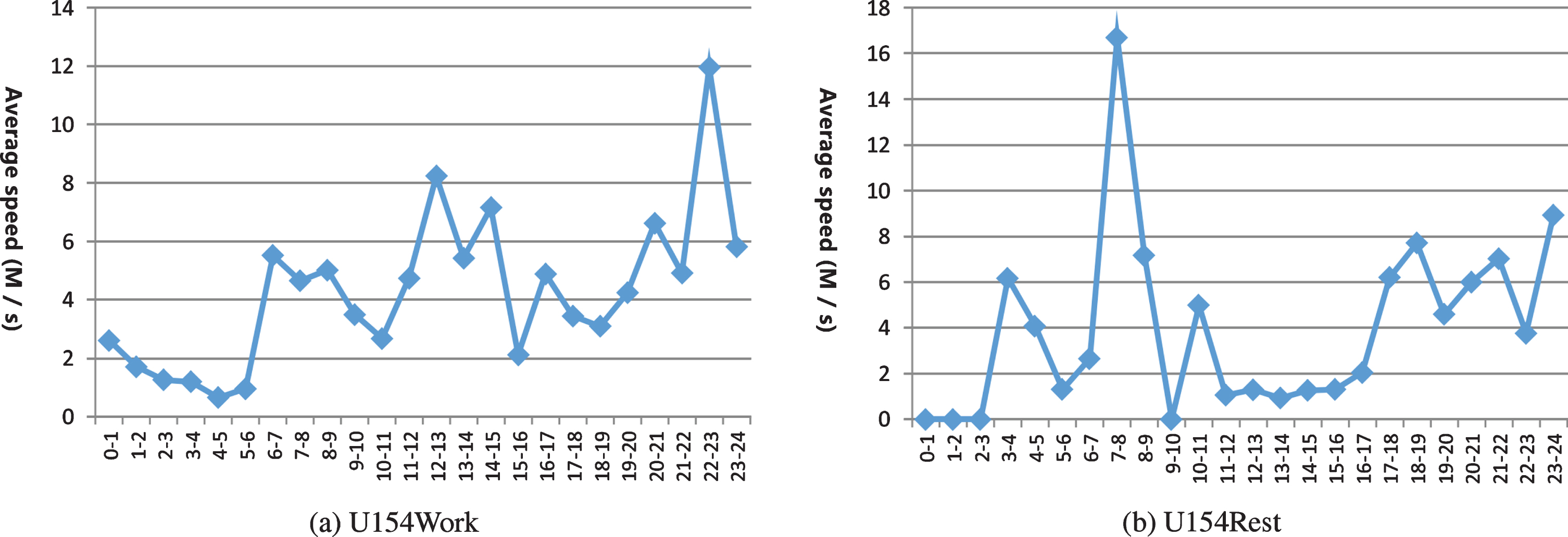
Fig. 5
The average speed of user164’s track data set over 24 time periods of a day.
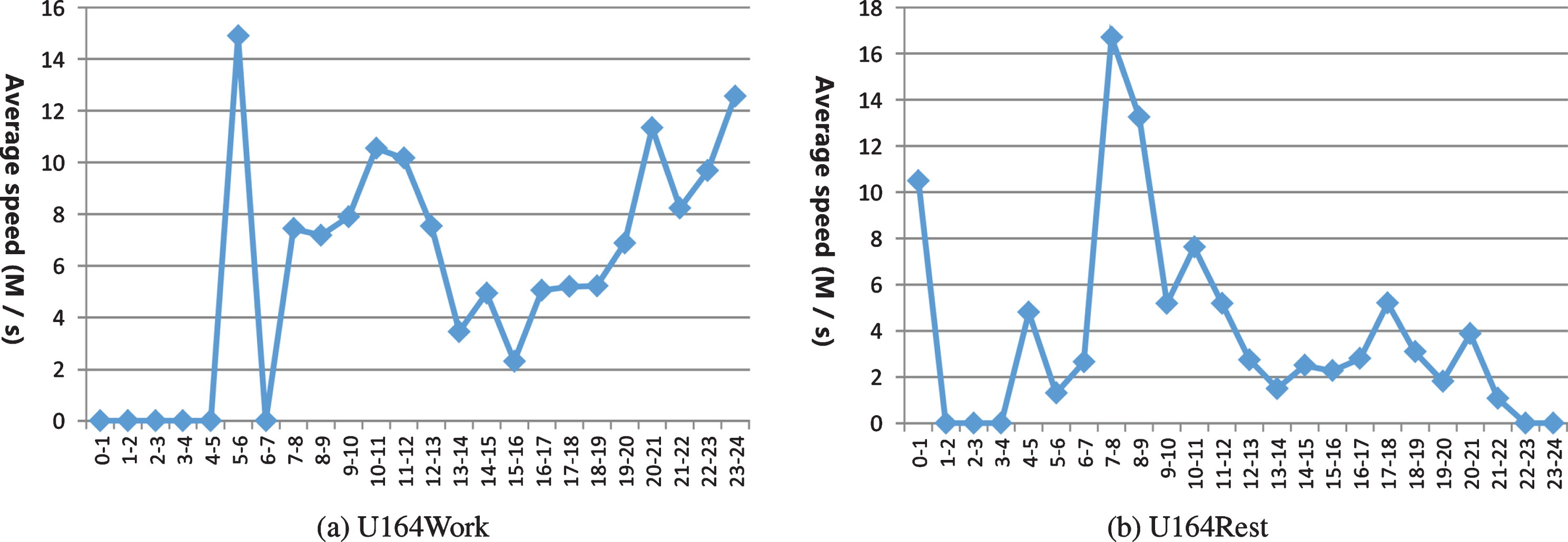
Fig. 6
The number of location points of user154’s track data set distributed in 24 time periods of a day.
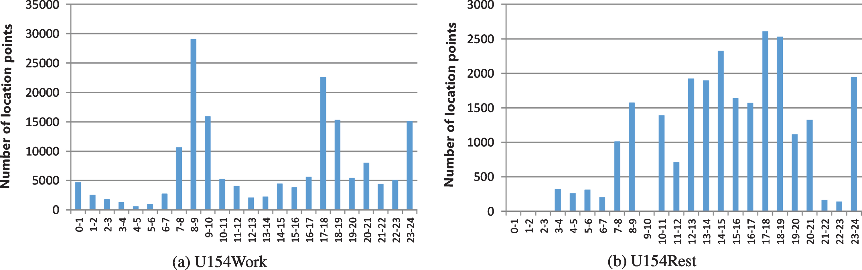
Fig. 7
The number of location points of user164’s track data set distributed in 24 time periods of a day.
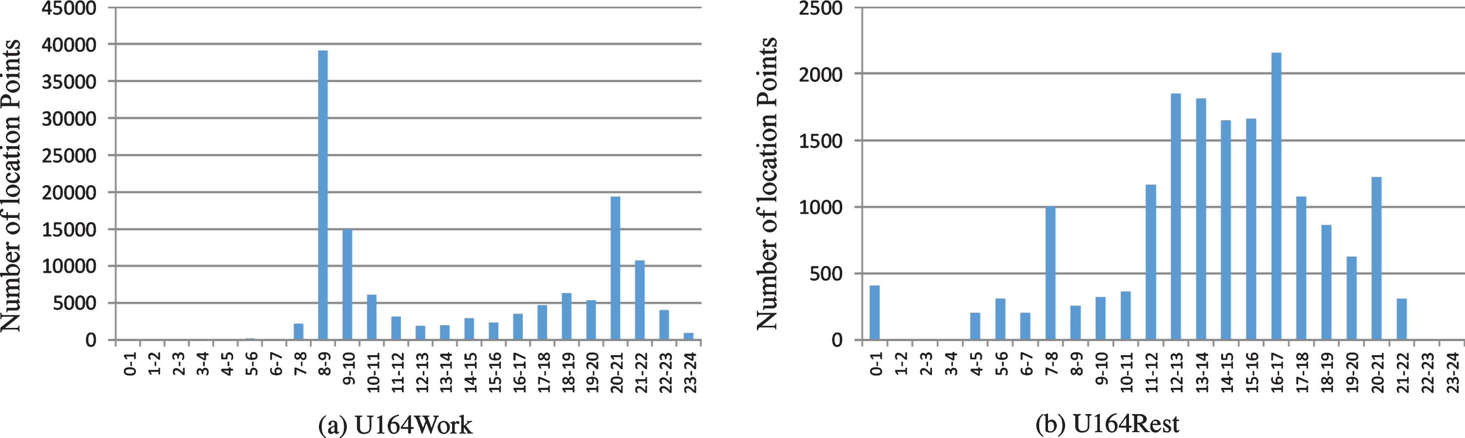
It can be seen from the travel track data of two users in 24 time periods every day during the working day of the year that the proportion of track number between 0:00 and 7:00, the number of sampling location points, moving distance and average speed are the smallest, indicating that the time period is a night rest time; the average speed between 7:00 and 9:00 is increasing rapidly, and the characteristics of outgoing behavior are obvious, so it is more likely to go to work. The number of sampling points between 9:00 and 17:00 is less, and the moving speed is relatively stable in other time periods except 12:00 to 13:00, indicating that the user may be in the workplace and have dining out during lunch break. From 17:00 to 19:00, the number of location points increases, and it is more likely to go to work. From 19:00 to 22:00, the number of location points and running distance did not change significantly, which may be at home or out for leisure. The movement speed from 22:00 to 24:00 first increased and then decreased, which reflected the possibility of going home at night.
It can be seen from the travel track data of two users in 24 time periods every day on the rest day of the year that the number of sampling positions and the moving distance between 0 and 7 are the smallest, indicating that the time period is the night rest time, which is similar to the track data of the working day. Although there is a high average speed situation, combined with the position point data and the proportion of track number, it may be due to the impact of individual abnormal travel track. Between 7 and 9, the number of points increased rapidly, the average moving speed first increased and then decreased, and the behavior of going out was obvious. The movement speed between 9:00 and 20:00 is relatively stable, which indicates that users have carried out similar activities here, and there is no significant change in lunch break and dinner time. It is possible that leisure activities have been carried out in an outdoor activity site. The average moving speed from 20:00 to 24:00 rises slowly, then rises rapidly and then falls, which reflects that there may be dining at night and going home from outside in this period. Compared with the results of track data analysis on working days, the early, middle and late travel time periods of rest days are different.
From the above track data analysis results, it can be seen that the work and rest time of the two users in the working day is relatively regular, and the early, middle and late travel division is relatively obvious; the rest day travel data is relatively small, and the travel time is mostly concentrated after 7 o’clock, and the travel characteristics of the whole day are not clearly distinguished.
The spatiotemporal trajectory data of residents’ travel can express the spatiotemporal relationship of individual behavior and reveal the spatiotemporal characteristics of individual daily activities. According to the detection results of outliers, we can analyze the abnormal behavior of individual travel. In the face of patients with COVID-19 and the prevention of epidemic situation, for each track, first calculate the direction of each track segment, and then obtain the corresponding sequence composed of track segments. Finally, the proposed method is applied to the real user’s daily travel trajectory data set. By detecting the outliers in the periodic travel trajectory data set of residents and analyzing the abnormal travel trajectory of residents, the possible causes for the abnormal behavior of COVID-19 patients mainly include the difference of travel purpose and travel time and the abnormality of traffic conditions. The results can be the residents’ travel Route recommendation and analysis of urban road traffic conditions provide valuable reference.
The representative path of the mobile object is obtained, and the periodic behavior mode of the mobile individual is found, and the travel characteristic information of the residents is further obtained. By using the time, direction, speed, shape, position and continuity features of each track to achieve more accurate measurement of track similarity, and based on the time length features of each track to optimize the initial center selection of track clusters, in order to achieve the ideal effect of track clustering. Then, taking urban residents’ commuting and routine route analysis as examples, the accuracy and performance of the proposed path clustering and location clustering algorithm are verified. It is helpful to realize the automatic acquisition of residents’ travel law information, and it is suitable for the geographic research fields such as the analysis of urban residents’ travel characteristics and the prediction of road congestion. It can provide an effective reference for the decision-making of urban planning and traffic management. And the relief can effectively relieve the epidemic prevention pressure of COVID-19.
5Conclusion
This paper mainly studies the spatiotemporal trajectory data mining method and its application in the analysis of urban residents’ travel behavior mode to solve the epidemic prevention and monitoring problem of covid19. Firstly, the inherent information and prior knowledge in trajectory data are fully studied, and the data model is constructed. Secondly, research data mining related technologies, innovate and design outlier detection methods, and analyze the abnormal travel routes on the personal travel trajectory data of city a residents, for example verification. It is used to identify various travel modes used in the user’s travel trajectory. Finally, based on the hot spot location mining method, this paper analyzes the spatial characteristics of urban residents’ travel according to the track data set of city a, and validates the detection of hot spot area by analyzing the key location of commuter route.
Based on the track clustering, this paper analyzes the continuity between the internal and external features and location points of the traditional track clustering method, and proposes a track clustering method based on multi feature similarity measurement. This method uses the characteristics of time, direction, speed, shape, position and continuity of tracks to measure the similarity between tracks, and optimizes the initial center selection of track clusters based on the characteristics of time length of tracks. The visual representation and experimental results show that this method improves the accuracy and stability of clustering results. Finally, on the real user daily travel trajectory data set provided by geolife project, the practicability of this method is verified through the analysis of residents’ routine travel routes, which provides the auxiliary decision-making basis for urban management and traffic planning.
Acknowledgments
This paper is supported by Undertake the R & D of key projects at municipal level and act as the R & D director. The project name is: A new platform for rapid screening and management of coronary pneumonia based on remote imaging. The project is mainly designed to be based on the Internet plus medical health mode, based on cloud image processing technology and health care big data standard. The software system is used to realize the CT remote screening and diagnosis of new type of coronary pneumonia, and to realize the multi-party expert consultation, to realize the disposal and monitoring of the whole process of the patient’s prevention and control, and to achieve two-way referral for the new type of patients with coronary pneumonia. The system forms a new clinical data center for patients with coronary pneumonia in the closed-loop processing of screening and control of patients with new coronary pneumonia, and data support is integrated with municipal health big data.
References
[1] | Benedetti F. , Beneventano D. , Bergamaschi S. , et al., Computing inter-document similarity with Context Semantic Analysis, Information Systems 80: (FEB.) ((2019) ), 136–147. |
[2] | Rahman M.A. , Hossain M.S. , Hassanain E. , et al., Semantic Multimedia Fog Computing and IoT Environment: Sustainability Perspective, IEEE Communications Magazine 56: (5) ((2018) ), 80–87. |
[3] | Yang Q. , A novel recommendation system based on semantics and context awareness, Computing 100: (8) ((2018) ), 809–823. |
[4] | Meng Y. and Qingkui C. , DCSACA: distributed constraint service-aware collaborative access algorithm based on large-scale access to the Internet of Things, Journal of supercomputing 74: (12) ((2018) ), 6418–6427. |
[5] | Kwak J. , Kim J. and Chong S. , Proximity-Aware Location Based Collaborative Sensing for Energy-Efficient Mobile Devices, IEEE Transactions on Mobile Computing 18: (2) ((2019) ), 417–430. |
[6] | Lai C.C. and Liu C.M. , A mobility-aware approach for distributed data update on unstructured mobile P2P networks, Journal of Parallel and Distributed Computing 123: (JAN.) ((2019) ), 168–179. |
[7] | Moghaddam S.K. , Buyya R. and Ramamohanarao K. , ACAS: An anomaly-based cause aware auto-scaling framework for clouds, Journal of Parallel and Distributed Computing 126: (APR.) ((2019) ), 107–120. |
[8] | Taleb S. , Hajj H. and Dawy Z. , VCAMS: Viterbi-Based Context Aware Mobile Sensing to Trade-Off Energy and Delay, IEEE Transactions on Mobile Computing 17: (1) ((2018) ), 225–242. |
[9] | Zhai Y. , Bao T. , Zhu L. , et al., Toward Reinforcement-Learning-Based Service Deployment of 5G Mobile Edge Computing with Request-Aware Scheduling, IEEE Wireless Communications 27: (1) ((2020) ), 84–91. |
[10] | Rahmani S. , Khajehvand V. and Torabian M. , Burstiness-aware virtual machine placement in cloud computing systems, Journal of Supercomputing 76: (1) ((2020) ), 362–387. |
[11] | Han H.Y. , Chen Y.C. , Hsiao P.Y. , et al., Using Channel-Wise Attention for Deep CNN Based Real-Time Semantic Segmentation With Class-Aware Edge Information, IEEE Transactions on Intelligent Transportation Systems PP: (99) ((2020) ), 1–11. |
[12] | Wang Y. , Liang J. , Cao D. , et al., Local Semantic-Aware Deep Hashing With Hamming-Isometric Quantization, IEEE Transactions on Image Processing 28: (6) ((2019) ), 2665–2679. |
[13] | Chang W.C. and Wang P.C. , Write-Aware Replica Placement for Cloud Computing, IEEE Journal on Selected Areas in Communications 37: (3) ((2019) ), 656–667. |


