
Big data analysis and empirical research on the financing and investment decision of companies after COVID-19 epidemic situation based on deep learning
Abstract
The novel corona virus pneumonia has brought pressure on economic development. Large and medium-sized companies will also play a key role in the recovery of growth after the outbreak. Therefore, it is particularly important to pay attention to the impact of the epidemic on large and medium-sized companies and on the investment and financing of companies. Firstly, the structure of the network model of data analysis is designed in this paper, including the design of the network level, the selection of the number of neurons in each level, the determination of the initial weight and other related parameters. According to the design of network structure, the evaluation model of investment and financing of listed companies is established. Python is used to preprocess the data and train the sample data. By comparing the data processed by two training methods, the optimal network classification model is selected. The experimental results show that the proposed method can improve the effectiveness of investment and financing decisions of listed companies.
1Introduction
At present, the fight against the epidemic has entered a critical period and its duration is still unknown [1]. In the short term, the first to be hit is large and small micro-enterprises, but with the spread of the epidemic, large and medium-sized listed companies with strong short-term risk resistance are bound to be hit. For example, the uncertainty of employees, the interruption of the supply chain and the decline in market demand may lead to difficulties in resuming work, production stagnation, profit decline and even losses; insufficient liquidity will bring credit and debt risks to enterprises. In the short term, large and medium-sized listed companies have a certain ability to resist “hit”, but in the medium and long term, these companies also face tremendous pressure, and once problems occur, they will have a huge impact on economic and social operations [2, 3]. All along, the development of large and medium-sized listed companies has played an important role in the stability of the entire economy and society. On the one hand, as the backbone of China’s economic development, large and medium-sized listed companies have obvious support and pulling effect on economic development; on the other hand, as the “leaders” and “wind vane” of industrial transformation and upgrading, they have a trend in the development of the industry Have a deeper and clearer understanding. The greater the capacity, the greater the responsibility. As the “ballast stone” of economic development, as well as the next step to resume production and lead growth, large and medium-sized listed companies shoulder major social responsibilities and have a long way to go. At the same time, some large and medium-sized listed companies in China have been integrated into the global industrial chain, and their healthy operation will also affect the smooth operation of the global economy. If the suspension of these enterprises will make the world economy feel chilled, it will accelerate the transfer of industrial chains from China, which will have a significant impact on the long-term development of our economy.
At the same time, we should objectively realize that the fight against the epidemic may turn into a stalemate [4–6]. Once this situation occurs, we must seriously consider the pressure on economic development and how to resume production while fighting the epidemic. Intensive and closed production may be a more realistic approach. Large and medium-sized listed companies have an advantage in this regard. Large and medium-sized listed companies will also play a backbone role in recovering growth after the outbreak. Therefore, it is especially critical to pay attention to the impact of the epidemic on large and medium-sized listed companies, especially on the investment and financing of listed companies.
2Historical data and materials analysis
According to relevant data, in 2016, the total operating revenue of B2B e-commerce platform of relevant enterprises was about 24.55 billion yuan, and the total scale was 21.45 billion yuan as of the third quarter of 2017, reaching 7.55 billion yuan in just three months, an increase of 17.5% year-on-year. In the same quarter of the same year, the amount of online shopping reached 1.44 trillion yuan, and the proportion of B2C continued to expand. Today, with the wide spread of Internet, the development of e-commerce not only plays an important role in the adjustment of industrial economic structure and the transformation of traditional enterprises, but also has an important guiding significance for the expansion of China’s “new economy” growth point after the 19th National Congress. In the future, the development of China and even the global economy is closely related to e-commerce.
Stock was born in the capitalist countries in the early 17th century. The emergence of stock is to solve the contradiction between the shortage of capital supply and demand and the expansion of business operation, and to obtain social financing through public issuance to the market. With the continuous emergence of this kind of joint-stock company established by raising share capital, the behavior of absorbing funds by way of stock develops rapidly, which also makes the development and maturity of stock market an inevitable trend. China’s stock was born in 1984 and entered the pilot period three months later. After more than 30 years of development, the stock has become an important member of the market economy. With the improvement of consumption level and income, more and more people regard stock investment as a part of daily financial management. However, due to various uncertainties in the stock market, it is easy to bring risks to the vast majority of ordinary investors, especially “retail investors”; at the same time, the volatility of the stock market also directly affects the stability and development of the whole national economy. Therefore, if we can establish a decision support model of stock quality evaluation and evaluate the stock quality of e-commerce listed enterprises reasonably, it will not only help the state and CSRC to better manage and check the stock, but also provide decision support for investors.
Li Chunwei collected 16 technical index data of “Dongfeng Motor” in 432 days, used BP modeling to predict the closing price in the next few weeks, and optimized the model by selecting the optimal index combination, which improved the accuracy of stock price prediction from 50% to 67% [7]. Han Wenlei [8] used probabilistic neural network to predict Shenzhen Stock Exchange Index, Shanghai Stock Exchange Index and Shanghai Stock Exchange 180 index, with the prediction accuracy of 82%, 77% and 82%, respectively. Peng Ying used the monthly average index data of Shanghai Composite Index from November 2004 to October 2005 to predict the index of November 2005 [9]. The model combined with GM (1,1), RBF and grey system and neural network was used to predict the index. The prediction errors were 2.58, 7.26 and 0.69 respectively. The accuracy of the combined model was the highest. Wang proved that epcnn’s prediction result is better than TSK system, TSK’s prediction effect is better than BPN, and BPN is better than multiple regression analysis [10]. The error of stock prediction of the four is 0.503, 2.16, 3.86 and 6.85. Liu Lei used the deep learning model to model the five indexes of three stocks and forecast the stock fluctuation at the next moment [11]. At the same time, compared with the results of traditional BP network model, the prediction accuracy of BP model was 60.43%, while that of deep learning model was 62.12%. Wu Shaocong compares and analyzes the results of stock time series prediction by the depth LSTM model and ARIMA model [12–16] and selects a mixed model combining the two to predict the short-term rise and fall trend of 12 stocks. The average absolute error predicted by LSTM model is 0.24, the average error predicted by the conventional ARIMA model is 1.35, while the error predicted by the improved DB-ARIMA model is reduced to 0.49, and the error predicted by the mixed model is about 0.33. The result is better than the first two.
3Deep learning
Deep learning is a kind of machine learning (ML) method. In essence, it is an ANN with multiple hidden layers. The early ANN model can’t solve the nonlinear problem. Until the discovery of BP algorithm in 1986, the nonlinear learning ability can be trained by the multi hidden layer neural network. Because of the limitation of early data scale, calculation scale and ability, the training and learning of parameters or weights of multi-layer neural network cannot achieve satisfactory results. Therefore, the development of neural network has been limited until recent years. With the rapid development of Internet and the explosion of information data, large-scale trainable data can support the learning and optimization of a large number of multi-layer neural network weights.
3.1Deep learning method
Deep learning methods are also divided into two categories: unsupervised learning and supervised learning. The difference between them is mainly to see whether the samples are labeled. Unsupervised learning means that the samples used for training do not have any labels, but directly model the data with many characteristics, so that the model can learn useful structural characteristics automatically. Unsupervised learning algorithms include clustering, association rules, CNN, etc. As the name implies, association rules are the important algorithms of data mining to discover the hidden relations between things from a large number of data. Clustering analysis is to solve the problem of classification, which is a common method in statistics. The most commonly used K-means clustering, especially for processing large data sets, is fast and efficient. CNN consists of two layers: feature extraction layer and feature mapping layer. The trained CNN can extract the local features and classify the image, and reduce the complexity of the model through the neural weights.
Supervised learning, generally speaking, is to classify the marked samples. GLM is the extension of linear model. According to the continuity of dependent variables, GLM can be divided into multiple linear regression and logistic regression. Decision tree can express the relationship between input and output intuitively. The key of the model design is to find a way to divide attributes. For example, the commonly used cart model uses Gini index to divide attributes. Random forest is the transformation of decision tree. It can not only speed up the learning process, but also improve the accuracy of classification. It has more advantages for processing a large number of input data. In practical application, the application method of unsupervised learning algorithm is far more than supervised learning, because in reality it is easy to collect a large number of unlabeled samples. To obtain labeled samples, it often consumes a lot of people, money and material resources. Especially in Internet applications, there are huge amounts of data, countless web pages can be used as unlabeled samples, and in-depth learning technology to increase data is the current development direction of artificial intelligence.
3.2BP neural network algorithm
BP neural network is the simplest deep learning model. BP algorithm is called error back propagation algorithm. In addition to the forward propagation, it also modifies the weight isometrically value through back propagation, so that the network error continues to reduce until it meets the expected output. The traditional BP back propagation process is as follows:
Let the expected output be Z’k, and define the global error between the expected output and the actual output as L:
(1)
Through the back propagation process, the error is expanded to the hidden layer as follows:
(2)
It can be seen from the above formula that the network error is a function of the weights wij and wjk. Therefore, by changing the weights of neurons, the error E can be changed:
(3)
(4)
In the formula, the negative sign represents gradient descent, ɛ represents rate, ɛ ∈ (0,1).
Through the above description of the analysis of the back propagation process, we describe the process of BP algorithm as follows, and Fig. 1 is the flow chart:
Fig. 1
Algorithm flow chart.
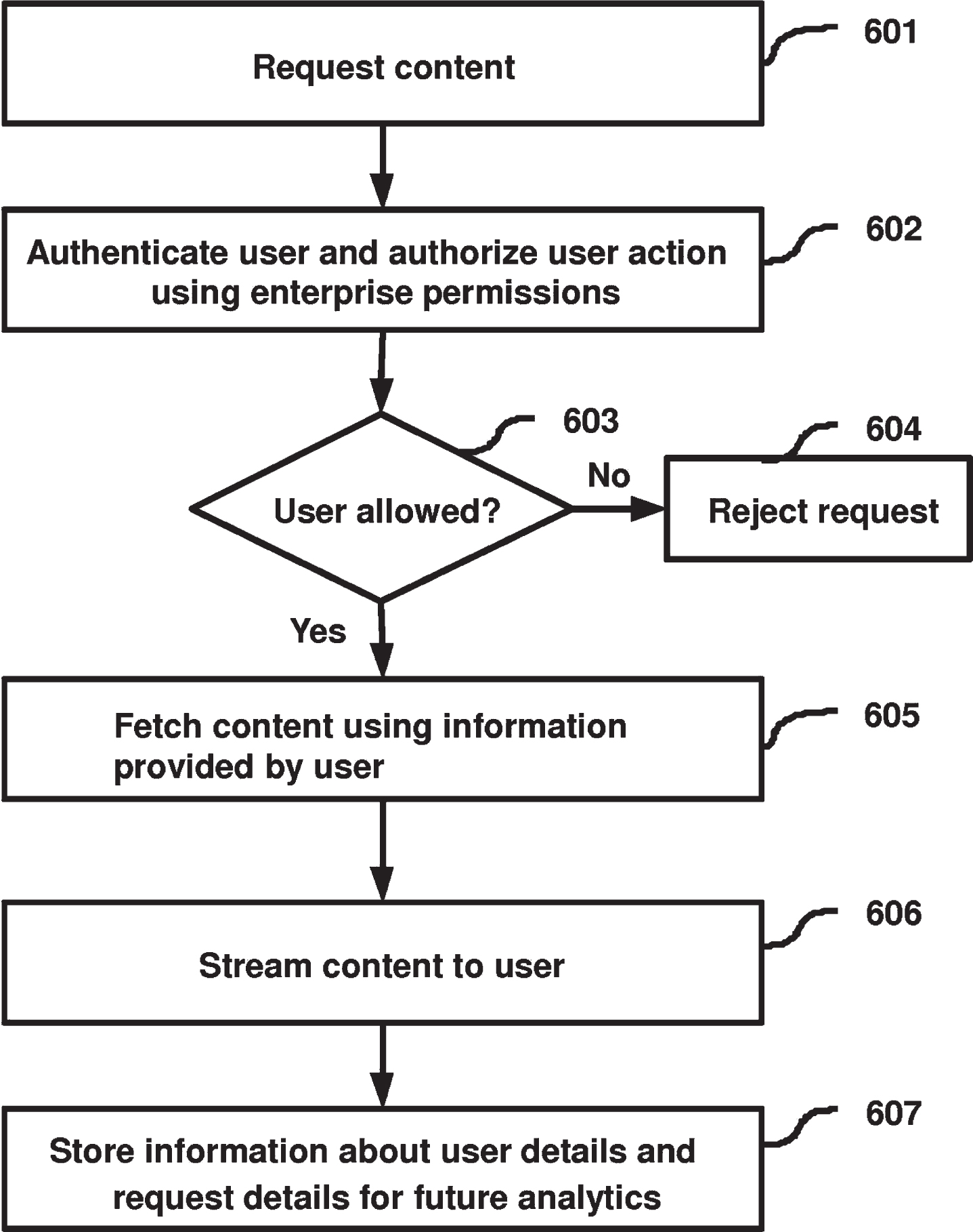
(1) Initialize network structure parameters, randomly set connection weight [–1,1], learning rate (0,1) and bias [0,1];
(2) Forward transmission: transfer the data into the network from the first layer to the last layer, calculate the output value according to formula 2.11, and compare the obtained value with the expected value. If there is a deviation, carry out step (3);
(3) In the reverse feedback process, according to the final error, it is transmitted to the first hidden layer, and the connection weight of each neuron is adjusted layer by layer by the following formula
It is calculated that the error of nodes in the same layer is δk, and the adjustment formula is:
(5)
The threshold value of the network can also be learned according to the weight correction process, assuming that the input signal is 1. Train the above process repeatedly until a satisfactory result is obtained.
4Application of deep neural network model in stock quality evaluation
Traditional stock or stock market analysis mainly evaluates stock prices, stock market fluctuations, etc. More often, it evaluates the general trend of stock price changes over a period of time. The methods include basic analysis, technical analysis, statistical analysis, etc. The traditional methods have greatly promoted the development of stock market research in the past. In recent years, with the continuous progress of computer technology, more and more methods have been applied to stock analysis, while more and more researches have been made on stocks using in-depth neural networks. It is evolved from the traditional artificial neural network. It is an artificial neural network with multiple hidden layers. The idea originates from the multi-level processing mechanism of human brain for input information. Deep neural network can learn the most significant characteristics of the original data through layer-by-layer training, which can well solve the problem of classification. Moreover, through layer-by-layer initialization, the training difficulty of neural network can be greatly reduced. The stock market is a complex dynamic system, containing a large amount of transaction data. The characteristics of neural network structure make it very suitable for analyzing stock market problems.
Input index data into the network model. Taking the 18 indicators of the largest shareholder’s shareholding ratio, listing time, 2014–2016 earnings per share, 2014–2016 dividend allotment, 2014–2016 asset liability ratio, whether to restructure in three years, number of legal proceedings, total share capital and circulating shares, issuance price, social responsibility report and key pollutant discharge units as input variables, 311 group sample data is used for training, 191 group sample data is used for testing, and the evaluation output is stock category. Table 1 shows the original data.
Table 1
The origin data
| Code | Industry | Total share capital | Tradable shares | State owned or not | Shareholding ratio of shareholders | Time to market | Issue price | Whether to increase shares | Dividend or not |
| 1 | 3 | 8,904,397,728 | 8,218,514,745 | 1 | 30.19 | 1,998 | 6.67 | 1 | 0.129 |
| 2 | 2 | 404,599,600 | 404,599,600 | 1 | 32.91 | 1,996 | 6.95 | 0 | 0.005 |
| 3 | 4 | 527,314,200 | 413,592,147 | 0 | 10.95 | 2,012 | 22. 00 | 1 | 0.046 |
| 4 | 3 | 3,111,443,890 | 2,702,903,890 | 0 | 41.01 | 2,008 | 20.31 | 1 | 0.355 |
| 5 | 2 | 400,980,000 | 341,130,000 | 0 | 32.73 | 2,012 | 25.50 | 0 | 0.074 |
| 6 | 2 | 22,102,656,925 | 22,089,726,225 | 1 | 52.14 | 2,000 | 4.18 | 1 | 0.027 |
| 7 | 2 | 170,112,265 | 170,009,195 | 1 | 22.36 | 1,996 | 8.80 | 0 | 0.074 |
| 8 | 2 | 3,150,029,146 | 2,718,950,221 | 0 | 38.95 | 2,010 | 15.00 | 1 | 0.355 |
| 9 | 2 | 1,506,988,000 | 1,239,816,011 | 1 | 34.16 | 2,009 | 60.00 | 0 | 0.428 |
| 10 | 2 | 6,015,730,878 | 5,970,491,879 | 1 | 18.22 | 1,996 | 2.50 | 0 | 0.775 |
| 11 | 2 | 562,413,222 | 562,413,222 | 0 | 42.58 | 2,003 | 4.30 | 0 | 0.022 |
| 12 | 3 | 1,730,795,923 | 1,453,377,893 | 1 | 35.02 | 2,004 | 3.00 | 1 | 0.077 |
| 13 | 3 | 46,679,118,459 | 46,679,118,459 | 1 | 25.15 | 2,010 | 3.10 | 0 | 0.027 |
| 14 | 3 | 957,936,440 | 603,240, 740 | 1 | 50.32 | 1,996 | 4.90 | 1 | 0.059 |
| 15 | 3 | 2,681,155,280 | 1,622,038,009 | 0 | 41.54 | 2,009 | 58.60 | 0 | 0.01 |
| 16 | 3 | 776,250,350 | 601,598,514 | 1 | 38.18 | 1,994 | 8.00 | 1 | 0.062 |
| 17 | 2 | 2,113,077,350 | 2,077,678,975 | 0 | 48.96 | 2,012 | 6.58 | 0 | 0.034 |
| 18 | 2 | 248,148,076 | 228,725,000 | 0 | 38.36 | 2,014 | 21.85 | 1 | 0.607 |
4.1The establishment of LSTM neural network evaluation and prediction model
The specific steps of evaluation and prediction model modeling are as follows,
(1) Firstly, the network structure and prediction accuracy are determined based on sample data and experience.
(2) Generally, there are two types of sample set: training sample and test sample.
(3) Select the appropriate network algorithm to train the model, so that the model can best fit the data of training period, this paper uses LSTM algorithm to train the network.
(4) Test the trained network with the test set data. If the result is ideal, use the model to evaluate the test set data; otherwise, adjust the model parameters and repeat the previous operation until the ideal output is obtained.
4.1.1Structure design of prediction model
For the neural network model, its network structure design can be said to be relatively “free”. In addition to the input and output layers need to be set according to data characteristics and objectives, the design of other values or parameters is basically based on experience, or through experiments to compare, without fixed procedures and steps. The level series of neural network is generally set according to the previous experience. A large number of studies and experiments show that the network with a small number of layers has strong generalization power, is easy to understand and extract features, and is conducive to implementation; However, the more the number of levels, the smaller the error of the network will be, which can improve the accuracy and complexity as well as increase the training time and speed of the model, which is likely to lead to over-fitting. Therefore, the number of levels can be set according to the effect to be achieved by the model. Generally, for a model with moderate data volume and high accuracy, a three-layer network can be selected. Andrey Nikolaevich Kolmogorov has proved that networks with more than three layers can fit any non-linear function and are also the networks most used in multi-layer networks. In this paper, the 10-layer depth LSTM network is used to build the stock quality evaluation prediction model.
The input and output layer parameters only need to be set according to the characteristics of index data. The input node matches the feature dimension, and the output node matches the target dimension. The sample contains 502 stocks, 18 data for each stock. Therefore, the number of input layer nodes m is set to 18, the last stock type is the format data of output data, and the number of output layer nodes n is set to 3.
The setting of the number of nodes in the hidden layer is the key and difficult point of the whole network structure design. There is no unified analytical expression to express it. The number of nodes has an important impact on the whole model effect. On the one hand, it affects the calculation ability of the network, on the other hand, it also affects the ability to approach the objective function. The more the number of nodes in the middle layer, the stronger the representational ability, which shows that the data storage ability of the network is strong, each node processes less data, and the accuracy is high; But once the number of neurons exceeds a certain degree, it will not only increase the learning time, but also affect the realization of the computer, similar to the problem of network level progression setting. Therefore, specific data need to be specifically analyzed and selected according to the characteristics of experimental data. Researchers usually determine the number of neurons according to previous experience or through continuous experiments. The commonly used determination method is called trial and error method, that is, several optional values are preset, then GridSearch algorithm is used to traverse the preset optional values, and the optimal value is selected by comparing the evaluation results. The trial-and-error method requires several basic formulas, and the calculated value can be used as the initial value of the number of hidden layer nodes. The specific formula is a s follows: s = log2 m; s = mn; s = m + n + a (s, m, n are the number of hidden layer, input and output layer nodes respectively, a is the constant; the number of input nodes finally selected through the experiment is 18; the number of hidden layer nodes is 50; the number of output layer nodes is 3.
4.1.2Selection of activation function
From the second chapter, we have a general understanding of the types of activation functions. S and T are S-type functions when the neural network is small. Tanh performs better than Sigmoid function, and Relu is the most widely used activation function.
Different from sigmoid function and tanh function, relu function is characterized by gradient unsaturation. The gradient calculation formula is: 1 x > 0. Therefore, in Backpropagation, the parameters can be adjusted quickly and the gradient vanishing process can be alleviated, so the calculation speed is fast. In the forward training, Relu does not need to calculate the index but only set the threshold value. This function can speed up the network computing speed. Therefore, Relu function is used in this paper.
Relu activation function (The Rectified Linear Unit) expression is:
(6)
Figure 2 below shows the basic graph of Relu function.
Fig. 2
Relu activation function.
4.1.3Other relevant parameter settings
There is great flexibility in setting the learning step size. In this paper, LSTM neural network algorithm is adopted, and the learning step length is updated automatically in training, so the initial value can be set according to previous experience. In this paper, the learning step is initialized to 0.001.
The error accuracy should be set according to the specific situation of the model, whether it requires high accuracy or strong generalization ability. The former can set the accuracy smaller, the latter can be appropriately larger, and the accuracy can be adjusted according to the results in the model training; in addition, the number of sample data and model neurons have an impact on the accuracy setting of the error. The more the training data, the larger the initial error, and the lower the training accuracy of the model. Because the larger the scale of the original data, the more variables in the model, the more variables lead to large errors. Set the error accuracy here to 0.01. The termination conditions of model training are mainly designed according to two aspects: first, when the model error meets the training accuracy requirements; second, when the model training time is too long or too many times, the process should be terminated. However, the first case shows that the training of network model is successful, while the second case shows that the artificial termination of network training due to time and number of times shows that the model does not meet the requirements of precision setting, so the model should be trained again. The key factor of unsuccessful network training is the unreasonable setting of initial connection weight, which makes the minimum value of model training deviate from the initial state greatly, or the excessive extreme value in the model may lead to too long training time. In this paper, the maximum number of training is set to 1000. When this value is exceeded, the time is too long and should be stopped.
5Simulation and implementation of evaluation results
5.1Raw data processing results
Some data after standardization is shown in Table 2.
Table 2
Some data after standardization
| Code | Industry | Total share capital | Tradable shares | State owned or not | Shareholding ratio of shareholders | Time to market | Issue price | Whether to increase shares | Dividend or not |
| 1 | 0.667 | 0.032 | 0.035 | 1 | 0.302 | 0.333 | 0.052 | 1 | 0.129 |
| 2 | 0.333 | 0.001 | 0.001 | 1 | 0.329 | 0.250 | 0.055 | 0 | 0.005 |
| 3 | 1.000 | 0.001 | 0.002 | 0 | 0.110 | 0.917 | 0.193 | 1 | 0.046 |
| 4 | 0.667 | 0.010 | 0.012 | 0 | 0.410 | 0.750 | 0.177 | 1 | 0.355 |
| 5 | 0.333 | 0.001 | 0.001 | 0 | 0.327 | 0.917 | 0.225 | 0 | 0.074 |
| 6 | 0.333 | 0.088 | 0.088 | 1 | 0.521 | 0.417 | 0.029 | 1 | 0.027 |
| 7 | 0.333 | 0.000 | 0.000 | 1 | 0.224 | 0.250 | 0.072 | 0 | 0.074 |
| 8 | 0.333 | 0.010 | 0.012 | 0 | 0.390 | 0.833 | 0.128 | 1 | 0.355 |
| 9 | 0.333 | 0.005 | 0.006 | 1 | 0.342 | 0.792 | 0.541 | 0 | 0,428 |
| 10 | 0.333 | 0.023 | 0.024 | 1 | 0.182 | 0.250 | 0.014 | 0 | 0.775 |
| 11 | 0.333 | 0.002 | 0.002 | 0 | 0.426 | 0.542 | 0.030 | 0 | 0.022 |
| 12 | 0.667 | 0.005 | 0.007 | 1 | 0.350 | 0.583 | 0.018 | 1 | 0.077 |
| 13 | 0.667 | 0.186 | 0.186 | 1 | 0.252 | 0.833 | 0.019 | 0 | 0.027 |
| 14 | 0.667 | 0.002 | 0.003 | 1 | 0.503 | 0.250 | 0.036 | 1 | 0.059 |
| 15 | 0.667 | 0.006 | 0.010 | 0 | 0.415 | 0.792 | 0.528 | 0 | 0.01 |
| 16 | 0.667 | 0.002 | 0.003 | 1 | 0.382 | 0.167 | 0.064 | 1 | 0.062 |
| 17 | 0.333 | 0.008 | 0.008 | 0 | 0.490 | 0.917 | 0.051 | 0 | 0.034 |
| 18 | 0.333 | 0.000 | 0.001 | 0 | 0.384 | 1.000 | 0.191 | 1 | 0.607 |
Input the standardized and sub boxed data into the network, and then according to the LSTM training steps, after repeated training, the number of hidden layer nodes is determined to be 50. The implementation process is written in Python language.
5.2The implementation of results in Python
(1) Introduction to Python
When using neural network to model and analyze problems, it involves a lot of mathematical calculation, such as differential solution, matrix calculation, etc., so we must use computer-aided processing. The training process of this paper is completed by python programming.
Python is a popular programming language in recent years, its language is simple and easy to understand, strong expansibility, and does not need a solid programming foundation. It is an open source software. Python can be used in combination with other languages such as C, C + +, Java, etc. packages written in other languages can be placed in Python programming platform for recognition and reading. It also provides a lot of convenient packages and expansion libraries, with built-in functions, which can quickly carry out the operation of numerical array, and can generate all kinds of exquisite charts.
In this paper, tensor-flow and python are used to complete the construction of LSTM model. Tensor-flow is an open-source framework developed by Google in 2015. Through the improvement of the first generation of deep learning system dist-belief, compared with dist-belief, tensor-flow has faster computing speed, can be applied to more platforms and has stronger stability. It uses the data flow graph to describe the calculation process, the calculation task is represented by the directed graph, the data processing is represented by the operations of the graph, and the flow is represented by the data flow direction. The lines in the flow graph represent the input and output of each node, and the whole flow graph represents the input, calculation and output process of high-dimensional array.
(2) simulation experiment steps:
- Defining file paths of storage models, training sets and test sets:
model_save_path = “./save/stock_rnn_save.ckpt”
train_csv_path = os.path.join (basic_path, “train_
data.csv”)
test_csv_path = os.path.join (basic_path, “test_
data.csv”)
- Define an LSTM single layer with “switch”:
def LSTM_cell ():
cell = rnn.LSTMCell (cell_num, reuse = tf.get_
variable_scope().reuse)
return rnn.DropoutWrapper (cell, output_keep_
prob = keep_prob)
- Define multi tier LSTM network:
LSTM_layers = tf.contrib.rnn.MultiRNNCell ([LSTM_cell () for _ in range (layer_num)], state_is_tuple = True)
- Using dynamic_ rnn function, which tells TF to build multi-layer LSTM network, and defines the output of this layer:
outputs, state = tf.nn.dynamic_rnn (LSTM_layers, inputs = input_rnn,
initial_state = init_state, time_major = False)h_state = state[-1][1]
- Define loss function, tf.train Some optimizers are provided, which can be used to train neural networks:
loss = -tf.reduce_mean (input_y * tf.log (y_pre))
train_op = tf.train.AdamOptimizer (learning_rate).
minimize (loss)
- Dealing with over fitting:
keep_prob = tf.placeholder (tf.float32, [])
input_x_after_reshape_2 = tf.reshape (input_x, [-1,
origin_data_col])
input_rnn = tf.nn.dropout(tf.nn.relu_layer(input_x_
after_reshape_2, W[’in’], bias[’in’]), keep_prob)
input_rnn = tf.reshape (input_rnn, [-1, origin_data_row, cell_num])
- Training LSTM neural network according to given parameters
sess.run (train_op,
feed_dict = input_x: train_x, input_y: train_y, keep_prob: 0.6, batch_size: _batch_size)
(3) Results of model operation after data standardization
After 5 times of training, the prediction accuracy of the evaluation model is 46%, which is quite different from the expected results. Therefore, it is necessary to increase the training times, and the prediction accuracy of 15 times of training is about 70%. The accuracy of the validation results is 77%, which is generally lower than 90%, indicating that the integration of the standardized data is not high.
(4) Model operation results after data discretization
After training the sample data of discretization with network model, the fitting degree of the model trained by the data of sub box operation is obviously higher than that of standardized operation, which can reach 92%, indicating that the evaluation model trained by discretization operation has high reliability.
(5) Actual forecast results
Select any 25 stocks involving e-commerce in the stock market, input the index data into the model, the results show that the prediction accuracy of the model is about 75%, indicating that 19 stocks are accurate in quality prediction. Compared with most scholars’ stock related forecasting models, the accuracy has been improved to a certain extent, and the model is feasible.
6Analysis of experimental results
According to the training results of the model test set, the model fitting error is about 0.08, which proves that the model is effective. The relative average error between the output value and the actual evaluation result is about 0.25, which improves the accuracy compared with the previous stock prediction. Due to many uncontrollable factors in the stock market, the general stock evaluation can not reach a high precision.
The results data after discretization is shown in Table 3.
Table 3
The results data after discretization
| general_capital | floatingcapital | stockholder | time_to_market | price | 2014_profit | 2015_profit |
| 0 | 0 | 0 | 0 | 0 | 0 | 0 |
| 0 | 0 | 1 | 0 | 0 | 0 | 1 |
| 0 | 0 | 0 | 2 | 0 | 0 | 0 |
| 0 | 0 | 1 | 2 | 0 | 1 | 0 |
| 0 | 0 | 1 | 2 | 0 | 0 | 0 |
From the above results, we can see that the average error of stock market prediction by scholars is about 0.36. The accuracy of the experimental model results is improved, so the experimental results show the accuracy and rationality of the stock quality evaluation model. Compared with the traditional single evaluation index, the index system established in this paper can basically reflect the influencing factors of all aspects of stock quality. Through the analysis of the impact indicators of stock quality, the quality, accuracy and comprehensiveness of the stock are improved to some extent. Investors do not need to carry out a series of complex calculations. They can see the quality of the stock intuitively according to the indicator system model, so as to consider investment. In addition, when using ANN to build evaluation model, attention should be paid to:
(1) The rise of domestic stock market is late, the regularity is not obvious enough, there is no sound market system to guarantee, and the securities investment market needs sound mechanism and standard rules to ensure the healthy operation. But China’s stock market is affected by many uncontrollable factors. At that time, political, economic and social factors will cause stock market fluctuations, especially policy changes or emergencies. At present, the evaluation and prediction model in this paper cannot solve these problems, and it needs further study by scholars in the future.
(2) It is more complex to examine the influencing factors of stock quality evaluation from various aspects and levels, such as foreign exchange, GDP, tax rate and other macro and micro factors. If we consider all the appeal factors comprehensively, the evaluation of stock quality will be more complex.
(3) Increase the selection of training samples. In this paper, only the three-year index data of 2014–2016 are selected for the selection of training samples. Compared with the data of 5, 10 or even longer years studied by professionals, the amount of data is less, which will also affect the accuracy of evaluation.
7Conclusions
For a long time, the stock market attracts a large number of investors with its high risk and high reward. At the same time, the stock market, as the “alarm” of market economy, attracts the attention of the government, investors and the general public. Therefore, the research on it has great theoretical and Application value. Since the birth of the stock market, there has been no lack of research on its fluctuation law and investment potential. There are many traditional research methods, such as fundamentals, technical level, sequence analysis, etc. because of the complexity and volatility of the stock market, it is difficult to build a simple and accurate model.
This paper expounds the structural design of the network model, including the design of the network hierarchy, the selection of the number of neuron nodes in each hierarchy, the determination of initial weights and the setting of other relevant parameters, and finally designs the structure of the stock quality evaluation model. The python language is used to show the results of data pre-processing and the training process of sample data. Through the training of the data processed by the two methods, the optimal network classification model is selected. Finally, the experimental results are analyzed and summarized, and the decision-making suggestions are given.
References
[1] | Liu Q. , Yang F. and Li C. , AWBING plus algorithm for generic object proposal generation, Journal of Intelligent and Fuzzy Systems 36: (6) ((2019) ), 1–17. |
[2] | Vraciu R.A. , Decision models for capital investment and financing decisions in hospitals, Health Services Research 15: (1) ((1980) ), 35–52. |
[3] | Devino G.T. , A Method for Analyzing the Effect of Taxes and Financing on Investment Decisions: Comment, American Journal of Agricultural Economics 53: (1) ((1971) ), 134. |
[4] | He Y. , Liao N. , Bi J. , et al., Investment decision-making optimization of energy efficiency retrofit measures in multiple buildings under financing budgetary restraint, Journal of Cleaner Production 215: (APR.1) ((2019) ), 1078–1094. |
[5] | Grichnik D. and Hisrich R.D. , Strategic and Investment Behaviour in the German and Israeli Venture Capital Industries: A Comparison with the USA, International Journal of Technology Management 34: (1-2) ((2006) ), 88–104(17). |
[6] | Migdalas A. , Applications of game theory in finance and managerial accounting, Operational Research 2: (2) ((2002) ), 209–241. |
[7] | Athanasios M. , Applications of game theory in finance and managerial accounting, Operational Research, 2002. |
[8] | Gentry W.M. , Debt, investment and endowment accumulation: the case of not-for-profit hospitals, Journal of Health Economics (2002), 21. |
[9] | Xing L. and Cheng P. , Real Option Analysis on Interaction Effects and Harmonizing Decisions between Investment and Financing, Systems Engineering 25: (4) ((2007) ), 59–63. |
[10] | Szabo S. , Jaeger-Waldau A. and Szabo L. , Risk adjusted financial costs of photovoltaics, Energy Policy 38: (7) ((2010) ), 3807–3819. |
[11] | Huhtala A. , Special issue on cleaner production financing, Journal of Cleaner Production 11: (6) ((2003) ), 611–613. |
[12] | Zhang X.Q. and Kumaraswamy M.M. , BOT-Based Approaches to Infrastructure Development in China, Journal of Infrastructure Systems 7: (1) ((2001) ), 18–25. |
[13] | Anderson J.M.M. , 1-d and 2-d system identification algorithms using higher-order statistics, Oil & Gas Journal (1992), 93. |
[14] | Danilova A. , Risk-Sensitive Investment Management, Quantitative Finance 15: (12) ((2015) ), 1–2. |
[15] | Kriger D. , Workshop 2: multi-modal infrastructure investment decision-making, Entomological News 96: (1) ((1997) ), 27–28. |
[16] | Guild P.D. , et al., Equity investment decisions for technology based ventures, International Journal of Technology Management, 1996. |


