
Security design and application of Internet of things based on asymmetric encryption algorithm and neural network for COVID-19
Abstract
During the period of COVID-19 protection, Internet of Things (IoT) has been widely used to fight the outbreak of pandemic. However, the security is a major issue of IoT. In this research, a new algorithm knn-bp is proposed by combining BP neural network and KNN. Knn-bp algorithm first predicts the collected sensor data. After the forecast is completed, the results are filtered. Compared with the data screened by traditional BP neural network, k-nearest-neighbor algorithm has good data stability in adjusting and supplementing outliers, and improves the accuracy of prediction model. This method has the advantages of high efficiency and small mean square error. The application of this method has certain reference value. Knn-bp algorithm greatly improves the accuracy and efficiency of the Internet of things. Internet of things network security is guaranteed. It plays an indelible role in the protection of COVID-19.
1Introduction
Since the outbreak of novel coronavirus in late 2019, 5 million 800 thousand cases have been confirmed worldwide, and 350 thousand cases have died. The mortality rate is 6.7%. With the novel coronavirus novel coronavirus infection and its spectrum of disease, the concept of new coronavirus infection has been emerging. Some of them even subverted some of the previous knowledge of infectious diseases. Novel coronavirus infection is a popular concept in recent years.
The key to the prevention and control of major public infectious diseases is time and efficiency, which reflects the efficiency of emergency response measures taken by health departments around the country to deal with major infectious diseases, and reflects the comprehensive treatment capacity of medical departments. With the increase of response time, the longer the virus is exposed in nature, the greater the potential risk of infection, and the number of infected people will increase exponentially. The diagnosis time of epidemic disease is defined as the time needed by patients from the onset to the diagnosis. Among the many time indicators of epidemic disease prevention and control, the diagnosis time is one of the most important indicators. Reducing community exposure risk is a traditional control measure and a very effective way to reduce the spread of infectious diseases.
Nowadays, the technology of Internet of things has come into the public’s sight, and the problem of network security has aroused widespread concern [1]. From the perspective of information technology innovation, the development of network security maintenance plan in combination with the needs of the times can play a fundamental role in the development of information technology [2]. At the same time, it is conducive to expanding the application of Internet of things technology. It can be seen that this thesis has the practical significance of exploration, and the specific content is analyzed as follows [3, 4].
The so-called Internet of things technology is a comprehensive technology to complete the exchange of things with the help of the Internet. It is based on Internet technology, providing reliable technical support for both field development and industry progress [5, 6]. The advantages of Internet of things technology are embodied in information integration, information authentication, information management and other aspects, and it has a wide range of applications, which can bring technical convenience to the application industry and promote the application industry to intelligent development. At present, the Internet of things system is composed of four parts, namely, the perception layer (data acquisition and processing), the transmission layer, the network layer (mobile communication and other networks), and the application layer [7]. There is a progressive relationship between all levels (subsystems), and the coordination and cooperation between subsystems make the Internet of things system run normally [8].
The Internet of things technology is used for intelligent operation, and only special maintenance is arranged in key links, for links without special maintenance [9]. The network attacker will take the opportunity to tamper with the program and make the intelligent operation disorderly [10]. The safety of personnel and materials is seriously threatened. Irreparable economic losses are caused [12, 13]. At present, the number of terminal node devices is huge and the types are complex [11]. Once the equipment protection is not in place, the network security cannot be guaranteed reliably, which ultimately affects the stability of information transmission [12, 13].
Radio frequency identification technology (RFID) relies on electromagnetic wave to share information. Due to the great influence of the outside world on the isolated transmission, the system security risk is increased invisibly. The limited degree of RFID resources is directly related to the protection ability of the system. If the limited resources are serious, the possibility of data information being tampered is relatively high, and the communication channel is blocked, which leads to a certain threat to the safety of readers and writers.
There is a close relationship between the number of communication ports and the capacity of the Internet of things system. Once the number of communication ports is small, the risk of the network system will be greatly increased, which can be reflected from the aspects of System Association, key management, system security, etc. Due to the large number of network devices in the system, the existing authentication methods only partially meet the needs of system management, resulting in the system association effect cannot meet the expected requirements, and then network system congestion occurs. Generally speaking, the integrated authentication method is more commonly used in the information encryption management. Once the Internet of things devices intervene in the key (key) formation, the resource utilization will be reduced. In addition, the network equipment obviously interferes with the complex encryption algorithm, and affects the speed of information transmission in varying degrees, resulting in the threat to the system security.
2KNN algorithm theory
K-nearest neighbor algorithm is mainly used to calculate the distance between the sample data to be tested and the total sample data, and then take the nearest sample data as the decision object. The most important part of KNN algorithm is the selection of K value, the way of classification decision and how to measure the distance between K values. Its basic idea can be understood as the relationship between an unknown sample data and K samples as the nearest neighbor sample set. When k samples satisfy a specific category, the unknown samples are determined to belong to the category similarity expression, which is measured by Euler distance, and the expression is shown in Equation (1).
(1)
Among them, as Vi = (vi1, vi2, …, vin) sample, the smaller the value of the expression is, the smaller the Euler distance is. The closer the nearest neighbor condition is, the greater the similarity between the two samples is. When KNN algorithm is used, it should be properly modified to Equation (2), indicating that only normal data values participate in the operation and are used for prediction.
(2)
For the selection and analysis of K value, K value has a great influence on the prediction results. The smaller K value causes the inaccurate classification and cannot reflect the practical significance of samples, while the larger K value will introduce irrelevant sample data, resulting in the decline of sample classification accuracy. The measurement of KNN algorithm can be expressed by mean square deviation, which is used to describe the distribution degree of samples, as shown in Equation (3), where x is the expected value, xi represents each sample data, and n represents the total number of data samples.
(3)
Next, we introduce K’s proximity algorithm.
K-nearest neighbor algorithm is one of the simplest algorithms in machine learning. The idea of k-nearest-neighbor algorithm is to find out the nearest (or most similar) k samples from the sample set, to see which type the vast majority of K samples belong to, and then classify x as this type.
Definition Vi = (vi1, vi2, …, vin) represents a sample, and the similarity calculation can be expressed by Euclidean distance (normalized by [0, 1]). The equation is as follows:
(4)
Obviously, the smaller the Euclidean distance is, the greater the similarity between the two samples is, and different weights can be given for the influence of neighbors with different distances on the sample. Then the weights are calculated as follows:
(5)
Where Simi represents the distance from the i of the K samples closest to the unknown sample X. Then the probability that unknown sample x belongs to class Cj is:
(6)
Where, x is the feature vector of the new sample, Sim(x, vi) is the normalized similarity, and y(vi, Cj) is the class attribute function, that is, if vi belongs to class Cj, then the function value is 1, otherwise it is 0.
In this paper, KNN algorithm is used to calculate the estimated value of abnormal attribute, and the Equation (1) is modified as follows:
(7)
Where vi is the sample with abnormal attribute value, vj is the normal sample, that is, the abnormal attribute does not participate in the calculation of distance.
The weighted average method is used to calculate the estimated value of the attribute. The equation for calculating the estimated value of the abnormal attribute is:
(8)
Where r indicates that the value of the r attribute is abnormal, and wj is the weight obtained by Equation (5).
3BP neural network
The model of BP neural network is composed of output node output model and hidden layer node output model. The neural network model has the characteristics of reverse error feedback and is a learning network with multi-layer transfer function. Its network architecture is shown in Fig. 1. It has three layers: input layer, middle layer and output layer. The input layer obtains the external information and transfers it to the middle layer. After the calculation of each neuron in the middle layer, it transfers it to the output layer. In the process of the middle layer, it can be processed by single hidden layer or multiple hidden layers.
Fig. 1
BP neural network structure.
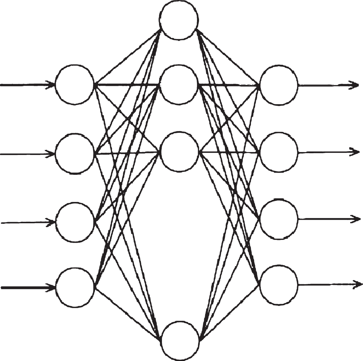
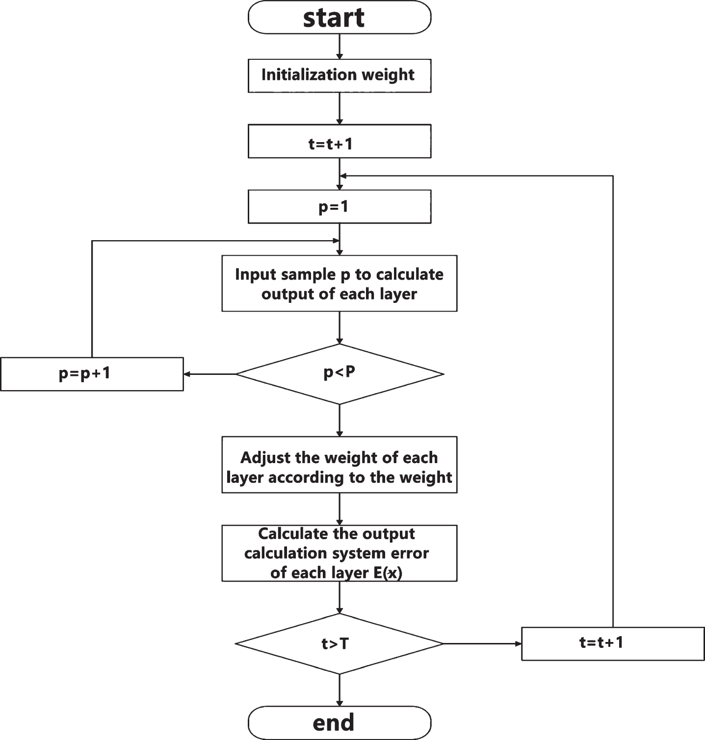
The weights of hidden layer nodes to output layer nodes are different. The connection weight coefficient is divided into two parts. The weight coefficient of input layer node Df connected to middle layer node Dm is set as wfm. The middle layer node Dm to output layer node Di is set as wmj, which indicates that when the output layer outputs information to the outside, the output value will be compared with the actual value. When the error cannot meet the system requirements, the weight value of each layer node will be adjusted and corrected by the way of back propagation. In the process of continuous modification of the weight value is also the process of neural network training and learning. In this learning process, the fastest descent method is used until the purpose of the training model is achieved, and the latter meets the preset neural network training times. The algorithm flow of realizing the neural network is shown in Fig. 2. The error calculation of the hidden layer and the mathematical model expression of self-learning are shown in Equations (9) and (10), respectively. In the process of self-learning, the sequence propagation direction and the back propagation appear alternately and repeatedly, while in the prediction model of the Internet of things, the variables in the network need to be normalized.
Fig. 2
BP neural network algorithm flow.
(9)
Tpi represents the expected output value of node i, while Opi refers to the actual output value for node i. M in Equation (10) is the learning factor, α is the momentum factor, and φ and o are the calculation error values.
(10)
BP neural network is a feed-forward neural network using BP algorithm. It not only has the structural characteristics of parallel processing, distributed processing and fault tolerance, but also has the functional characteristics of self-learning, self-organization and self-adaptive. It has the abilities of associative memory, nonlinear mapping, classification, recognition and prediction, optimization calculation, knowledge processing, etc. It does not need to analyze the specific relationship of the relevant factors, through a certain sample of learning and training, it can summarize its own complex internal laws, so as to predict. The basic unit of neural network is neuron, and the output equation of each neuron is:
(11)
Where
(12)
BP neural network adjusts the weight and threshold through the form of back-propagation error, and the error calculation equation of output neuron is:
(13)
where Tj is the expecting output value.
The error equation of hidden layer neurons is as follows:
(14)
The weight increment Δ Wij is:
(15)
The threshold increment is:
(16)
BP neural network can achieve the goal of training and achieve the function of classification and prediction by constantly adjusting the weight and threshold.
4Traditional forecasting methods of Internet of things
The exponential smoothing prediction model is first proposed by Robert Brown. The model follows the characteristics of time series, and the prediction of things should meet the regularity and stability. On the time scale, the results that are closer to each other are more likely to have greater weight in the future prediction model. In combination with the exponential smoothing value of each time series in the model and the previous exponential smoothing value of a short period of time, the reference weighted method is used to average. The weighted average of the primary index or the secondary index can be used to predict by using the exponential smoothing value. The mathematical models of the primary and secondary exponential smoothing are shown in Equations (17) and (18).
(17)
(18)
Among them, St represents the primary exponential smoothing value, α represents the weight, the data in each time period is yt, and the data to be predicted in the next time period is yt+1, while the coefficient weight value of the secondary exponential model is calculated according to Equation (19), and the predicted value of the secondary exponential smoothing is calculated by measuring these coefficients.
(19)
At present, the prediction method of this model is relatively simple, which mainly uses the value in a period of time series affected by periodicity to budget the possibility of time occurrence in the future. The expression of its mathematical model is shown in Equation (20). By moving average method to reduce the effect of uncertain fluctuations, the prediction value is wt +1, and N represents the total number of samples.
(20)
Grey prediction model is a prediction method between white box prediction and black box prediction. Compared with all obvious elements in white box and unknown elements in black box prediction, grey prediction method mainly aims at some unknown and known elements. On the time scale, the event sequence has n elements, which are represented by Equation (21). As time passes, the event state accumulates, and the new sequence value is represented by Equation (22). The equation is shown in Equation (23).
(21)
(22)
(23)
The parameter μ indicates the endogenous control grey value and α is the development grey number. The mathematical expression of the prediction model is shown in Equation (24), where X1 (k + 1) is the prediction value.
(24)
k = 1,2,3, ... ,n
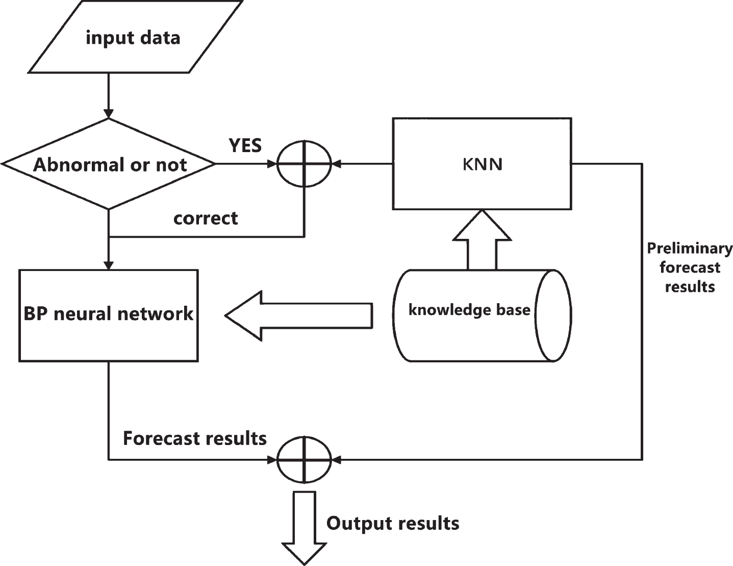
The prediction model of KNN algorithm combined with BP neural network is shown in Fig. 3. The prediction process of the prediction model is to input the input data into the judgment window first. When there are outliers, they will be corrected by KNN algorithm, and the missing data or outliers will be replaced by KNN algorithm estimates. Then the modified value is transferred to BP neural network for learning and training, and a model based on the correct input data is established. BP neural network relies on the data in the knowledge base for continuous training, and finally gives the predicted value.
Fig. 3
BP neural network prediction flow chart combined with KNN.
To describe the algorithm of training sample data flow, first assume that the original sample of input data is W, the number is N, and finally get the training sample is WKNN. In mathematical processing, the initial sample W can be divided into two combinations W1 and W2. For the natural number of variable i satisfying i ∈ (0, N), for each Wi. Check whether the data is normal. If it is abnormal, remove it and put it into W2 abnormal data set. If it is normal, put it into W1 normal data set.
For the abnormal data set W1, the method of KNN is used to select K nearest neighbor sample data in the normal data set W1, and then the weight coefficient of K nearest neighbor is calculated to get W2KNN. After processing, the set is combined into WA, after training, the new sample is predicted, and the new set is input into the BP neural network for model prediction. At this time, predict the result for the new input sample Y. Assuming that μ1 is the preliminary prediction probability of the KNN method, when the sample Y satisfies the correction condition, K nearest neighbors are selected from WA, and after calculating the weights of the replacement outliers, a new set YA is formed, and the probability that the sample YA belongs to a category is P1 Then the BP neural network is used to predict YA, and the category with the largest probability value in P2 is obtained. α and β represent the confidence weight coefficients predicted by KNN and BP neural network respectively, which should satisfy α+β= 1.
KNN-BP neural network prediction model can be divided into two processes: the processing of training samples and the prediction of new samples. The first process corrects the value of abnormal attributes of abnormal samples in the training samples. The second process checks whether the new samples are abnormal and uses the new samples for prediction.
The processing of training samples is as follows:
Input: original training sample V, N;
Output: after treatment training sample VA; which is shown in Figs. 4 and 5 for the flow.
Fig. 4
Process 1.
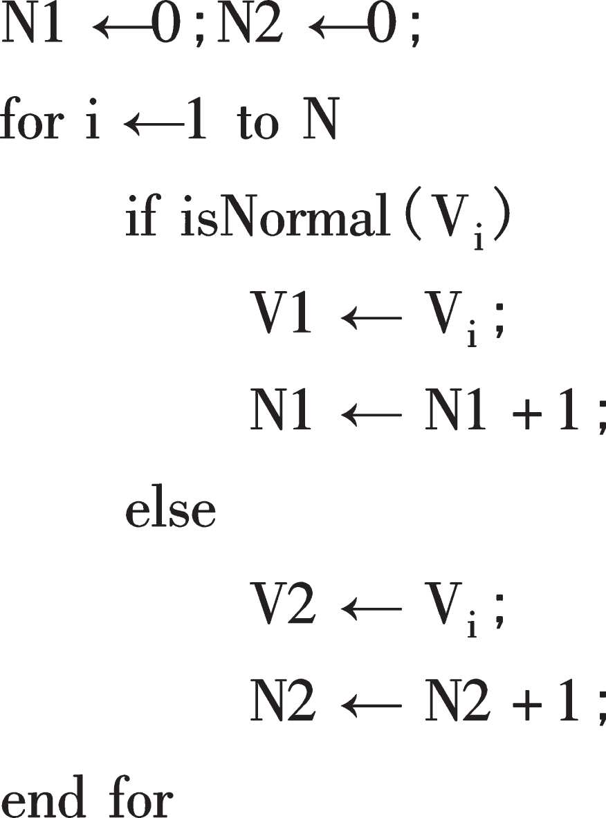
Fig. 5
Process 2.
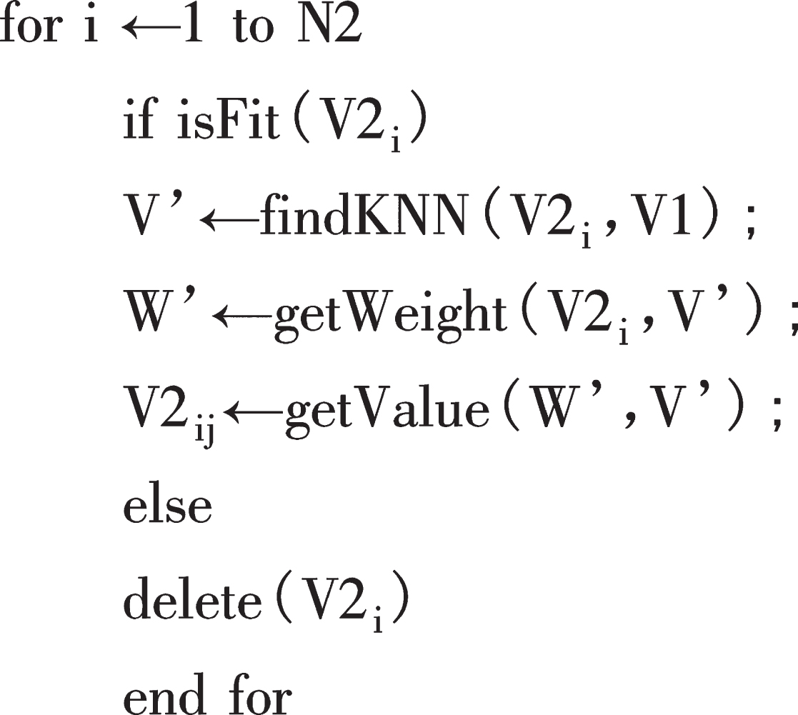
In the above process, it is necessary to judge whether the abnormal samples meet the correction conditions. Only when the number of abnormal attributes is less than the set number r, can the correction be performed. Otherwise, the data will be directly discarded. After processing the training samples, the BP neural network can be used for training. After the training, the new sample can be predicted, which is shown in Fig. 6.
Fig. 6
Process 3.
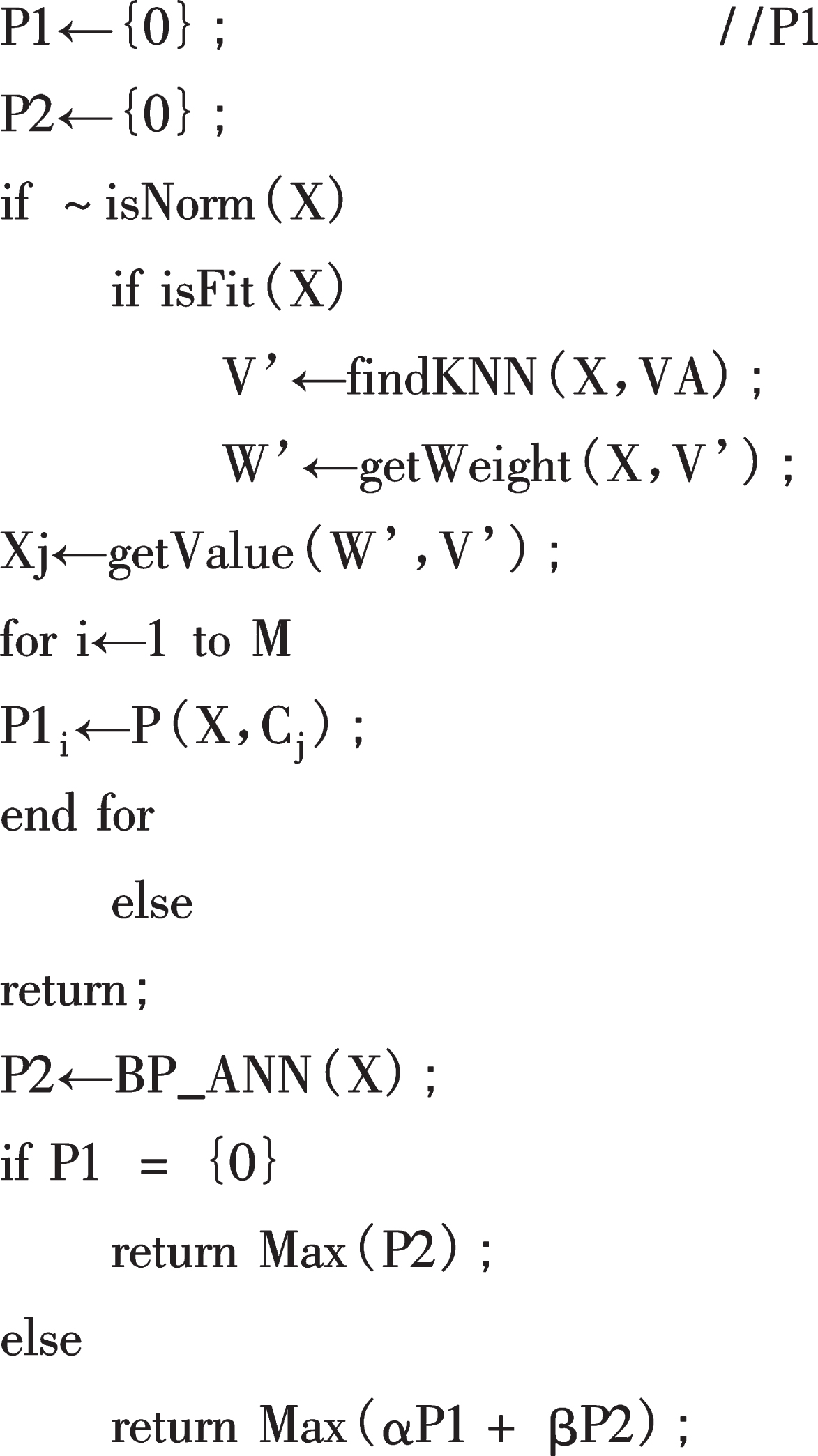
In the above process, α and β represent the confidence weight of KNN and BP algorithm prediction results respectively, where α + β= 1. In addition, when the original training data set is large, the first process can be skipped, and the abnormal samples can be deleted directly instead, and the normal samples can be used as the training set. For the two processes of searching K-nearest neighbors, when the sample data set is large, a certain number of sample set S can be randomly selected according to the classification result category proportion, and then K-nearest neighbors of the sample can be found in S to save computing resources. In this model, the training data set needs to be stored in the knowledge base for the convenience of prediction.
5Experimental results
The experimental data comes from the data collected by two groups of wireless sensors located in different places (two different directions outside a building). The data is transmitted back to the gateway through the base station multi hop. Each group of data includes four data: light, humidity, temperature and atmospheric pressure. In the experiment, the collected wireless sensor data plus the collected time period is used as the input parameter. Its format is: (time, illumination 1, temperature 1, humidity 1, pressure 1, illumination 2, temperature 2, humidity 2, pressure 2). Using such input data to predict the weather conditions of the area where the wireless sensor is located, the prediction results are sunny, cloudy and rainy days. The amount of data collected is large. In this experiment, the method of random sampling is used to use some of the data. When the number of abnormal attributes is more than 3 (r = 3), the sample is useless. When looking for k nearest neighbors of the sample, the search range is a sample set composed of 100 pieces of data randomly selected from the training sample data set in proportion. In the experiment, K is set as 5, α is set as 0.2, β is set as 0.8.
The experiment is divided into two groups, one is when the training data set is large (1000 pieces). For the new samples with 1, 2 and 3 attribute anomalies, this method is compared with the prediction using only BP neural network (the outliers are replaced by the average value of the attribute in the region).
In the second group of experiments, when there are less prediction samples (100 samples) and a small number of abnormal samples, the comparison between the prediction results of this method and the prediction results of BP neural network method is also made when there are 0, 1, 2 and 3 attribute abnormal samples in the new samples. The number of test samples in the experiment is 100, and the results of the two groups of experiments are shown in Tables 1 and 2:
Table 1
Prediction results of the model with a large number of training data sets
| Number of models /exceptions | 1 | 2 | 3 |
| KNN-BP | 0.94 | 0.93 | 0.93 |
| BP | 0.84 | 0.81 | 0.77 |
Table 2
Prediction results of the model with a small amount of training data set
| Number of models /exceptions | 0 | 1 | 2 | 3 |
| KNN-BP | 0.93 | 0.91 | 0.93 | 0.92 |
| BP | 0.89 | 0.87 | 0.84 | 0.78 |
Table 2 shows the training and prediction results of KNN-BP model and common BP model in this paper when there are few training data samples. In the experiment, a small number of abnormal samples in the training data set are replaced by KNN estimated value and attribute empirical average value respectively. Table 1 is the prediction results of the two models after deleting the abnormal data in the training samples directly when the training data samples are large.
It can be seen from the experimental results that BP neural network has strong prediction ability and certain fault tolerance ability. Its prediction ability is related to the integrity of training samples, the proportion of normal data of training samples, and the integrity of prediction data. When the number of training samples is small, the KNN-BP model is more reasonable to replace the abnormal attributes of the abnormal data in the training set, which makes the prediction accuracy of the model higher. On the other hand, when the attributes of the test samples are abnormal, the general BP neural network model shows obvious inadaptability, the prediction accuracy is obviously reduced, and the KNN-BP model shows high stability. When the number of abnormal attributes is within a certain range, it can still maintain a relatively high prediction accuracy, which significantly improves the adaptability of the prediction system, especially suitable for the application scenarios where wireless sensor networks are prone to data loss or abnormal in the Internet of things environment. It is worth pointing out that the sensor in the Internet of things application environment collects a large amount of data, which can provide a large number of data samples for the prediction model. Therefore, the first group of experiments are more common in the Internet of things, and it is more appropriate to use the KNN-BP prediction model in this paper.
6Conclusions
During the protection period of COVID-19, the security of Internet of things is concerned. The characteristics of Internet of things wireless sensor data are collected. The traditional BP prediction model is analyzed, and a method combining BP neural network with KNN algorithm is proposed. K-nearest-neighbor algorithm has good data stability for adjusting and supplementing outliers, and improves the accuracy of prediction model. Compared with the traditional BP neural network algorithm, this method has the advantages of high efficiency and small mean square deviation. To ensure that the sample data value is not lost or mutated has the best predictive significance. For the sample data without attribute experience, it is often difficult to calculate the empirical prediction value. However, the prediction model in this paper has more obvious algorithm advantages. This method has certain reference value in practical application. In the next research, we will continue to optimize the prediction model, for example, we can introduce deep learning to train the model, and use information fusion technology to further improve the prediction accuracy and efficiency of wireless sensor networks in the Internet of things environment. During the protection period of COVID-19, the security of the Internet of things is realized through the algorithm.
Acknowledgment
This paper is supported by Natural Science Foundation of Science and Technology Department of Hunan Province titled “Research on Key Technologies of mobile learning platform based on Wechat applet” (No.: 20191j70086).
References
[1] | Golgiyaz S. , Talu M.F. and Onat C. , Artificial neural network regression model to predict flue gas temperature and emissions with the spectral norm of flame image, Fuel 255: (NOV.1) ((2019) ), 115827.1–115827.11. |
[2] | Xu Y. , Li D. , Wang Z. , et al., A deep learning method based on convolutional neural network for automatic modulation classification of wireless signals, Wireless Networks 25: (7) ((2019) ), 3735–3746. |
[3] | Schran C. , Behler J. and Marx D. , Automated Fitting of Neural Network Potentials at Coupled Cluster Accuracy: Protonated Water Clusters as Testing Ground, Journal of Chemical Theory and Computation 16: (1) ((2020) ), 88–99. |
[4] | Sohn W.B. , Lee S.Y. and Kim S. , Single-layer multiple-kernel-based convolutional neural network for biological Raman spectral analysis, Journal of Raman Spectroscopy (2020), 51. |
[5] | Kannan G. , Gosukonda R. and Mahapatra A.K. , Prediction of stress responses in goats: comparison of artificial neural network and multiple regression models, Canadian Journal of Animal Science (2020), 100. |
[6] | Komeda Y. , Handa H. , Matsui R. , et al., computer-aided diagnosis (cad) based on convolutional neural network (cnn) system using artificial intelligence (ai) for colorectal polyp classification, Endoscopy 51: (04) ((2019) ). |
[7] | Kim H.G. , Hong S. , Jeong K.S. , et al., Determination of sensitive variables regardless of hydrological alteration in artificial neural network model of chlorophyll a: Case study of Nakdong River, Ecological Modelling 398: ((2019) ), 67–76. |
[8] | Solaiyappan M. , Weiss R.G. and Bottomley P.A. , Neural-network classification of cardiac disease from 31P cardiovascular magnetic resonance spectroscopy measures of creatine kinase energy metabolism, Journal of Cardiovascular Magnetic Resonance 21: (1), 2019. |
[9] | Yuan N. , Dyer B. , Rao S. , et al., Convolutional neural network enhancement of fast-scan low-dose cone-beam CT images for head and neck radiotherapy, Physics in Medicine and Biology 65: (3), 2019. |
[10] | Narita E. , Honda M. , Nakata M. , et al., Neural-network-based semi-empirical turbulent particle transport modelling founded on gyrokinetic analyses of JT-60U plasmas, Nuclear Fusion 59: (10), 2019. |
[11] | Nowrangi R. , Kalantari J. , Kiang S. , et al., Abstract No. 481 Training a convolutional neural network to detect refractory variceal bleeding in cirrhotic patients, Journal of Vascular and Interventional Radiology 31: (3) ((2020) ), S213. |
[12] | Rodríguez U.B. , Vargas C.Z. , Gonçalves M. , et al., Bayesian Neural Network improvements to nuclear mass equation and predictions in the Super Heavy Elements region, EPL (Europhysics Letters) 127: (4) ((2019) ), 42001. |
[13] | Zhang T. , Wang J. , Chen X. , et al., Can Convolutional Neural Network Delineate OAR in Lung Cancer More Accurately and Efficiently Compared with Atlas Based Method, International Journal of Radiation Oncology Biology Physics 105: (1) ((2019) ), 542–543. |


