
An intelligent strategy for faults location in distribution networks with distributed generation
Abstract
The exact location of faults in the electrical distribution systems is a problem that affects not only the users, but also the companies providing the electric service. With greater time invested in this period, the losses due to unbilled energy and inconvenience to users increases, thus decreasing the quality of service. One of the causes of the growth in time is the misunderstanding that might exist in the localization systems that act under the presence of distributed generation sources in the distribution networks. In this sense, the present research develops an intelligent diagnosis of faults in distribution systems with distributed generation. Three stages are defined: Identification of the type of fault, the location of the zone, and the exact point of fault. A mixed method based on artificial intelligence and mathematical algorithms is applied. Eleven different types of faults that can occur in a distribution system are considered with six different values of fault resistances ranging from 5 to 30 Ω. The errors found are less than 2% in the location of the fault point with robustness to variations in the load and the penetration of distributed generation.
1Introduction
Power Quality (PQ) has become a topic of interest to electric service users. Given the obvious importance for today’s society, electricity must be supplied as a service with quality parameters, that is, in a reliable, safe, and sustainable way, without sacrificing the lives of users, animals, plants and equipment and, simultaneously, must be available whenever the user needs it.
The distribution of electric energy must be performed in such a way that the user receives a continuous service, without interruptions, with an adequate voltage value that allows the electrical equipment to operate properly. However, the Electrical Distribution Systems (EDS) are not immune to power outages caused by faults. The time of an interruption depends on the fault detection by the protection device, its opening and clearing, the location of the fault and the repair necessary to restore the service. The location process depends on two main factors like the topology, i.e. length of the feeder and number and length of the branches; the geographic characteristics of the area where it is located and can make the fault location difficult [1, 2].
The integration of the Distributed Generation (DG) into the conventional EDS modifies the amplitudes of the fault signals (voltage and current), which significantly affects the accuracy of the fault localization algorithms [3]. For this reason, it is important to deal with this problem when there is presence of DG in networks [4].
Algorithmic methods were used to solve this problem with the use of DG. These methods depend on the network model and the error in the fault location increases significantly with the increase in power fed by DG sources in the EDS [5]. The authors of [6] use the impedance-based method to locate faults in EDS with presence of DG. The technique is validated in the IEEE circuit of 34 nodes considering different types of faults that can be presented with resistances between 0 and 40 Ω and penetration of DG between 5 and 50%. The results show estimation errors of less than 2%.
In [7], the author indicates that the methods based on the impedance are influenced by the fault resistance and by the distance between the fault and the measurement point. With greater resistance and fault distance, the error in the estimation is greater. In general, the accuracy of impedance-based methods depends on the parameters of the line, its characteristics, and the load value. The error in the localization of these methods is also affected by the complexity of the network, characterized by unbalanced systems, multiple sides, and different fault resistances. For faults with multiple estimated distances, the state of the protection devices is commonly used to identify the actual location. However, for a EDS that is not equipped with the online status of protection devices, the problem of multiple estimation could not be solved [8]. These methods provide accuracy although with multiple estimation at fault location [9].
In [10], the authors locate faults in EDS with presence of DG using Artificial Neural Networks (ANN) with the standard backpropagation approach. In this method, the training data is based on the current fed by each DG during the fault. Therefore, the accuracy of the method is highly dependent on the number of DG sources in the system. The main problem of ANNs is their high dependence on the quantity and quality of the data trained to produce a well-trained algorithm. A limited information or inaccuracy affects the performance of the algorithm to correctly identify the location of the fault. This problem occurs in EDS with limited information resulting from an insufficient number of monitoring devices [8].
Support Vector Machines (SVM) have been used to locate faults in EDS with DG. These are based on patterns represented by voltage and current measurements in the substation and DG sources. This technique presents greater robustness when the number of DG sources in the network is increased [11].
In [11] authors present the application of the SVM to diagnose faults in EDS with the presence of DG. The proposed approach is based on the three (3) voltages and phase currents that are available from all sources, i.e. at the substation and the DG connection points. The proposed methodology is illustrated in a distribution feeder of the 132/11 kV substation in India with loads at different locations and several DG sources. The proposed fault localization scheme can identify the type of fault, the location of the fault section, and the fault impedance. The result of the simulation shows the satisfactory performance in terms of classification and regression. The accuracy of the classification for the fault line was 100, 99.95, and 92.06%, with three (3) sources of DG, two (2) DG and one (1) DG, respectively. For any changes in the system topology, the SVMs must be re-trained for their application. In addition, with a greater number of DG sources, the approach becomes more robust.
Finally, the authors of [8] indicate that a research can be done in the future to improve existing methodologies that consider the interconnection of DG in the EDS that can result in advances in the issue of fault localization. The authors [12] confirm the need to study the problem of locating faults in EDS with DG, with new methods and with the combination of traditional methods. Similarly, the authors [13] indicate the importance of conducting investigations in locating faults in EDS with parallel approaches, i.e. combining different methods. In [14] they state that in the future the investment of electricity generation will be in DG which will allow to improve the voltage profiles in the EDS in direct proportion to its penetration, however, it clearly increases the levels of fault current and alters individual contributions from generation sources. This requires more research to avoid the loss of security and reliability of the system. In [18] the authors propose that the issue of fault localization in EDS will be deepened in models based on AI. This research is different to other developed in the area because it considers the presence of DG sources and the combination of different fault localization techniques. The benefits of this strategy can be evaluated considering the results of the accuracy in the location of the faults. The number of variables used, and their sensitivity analysis of the parameters involved will allow to measure the robustness of the strategy developed.
2Proposed methodology
2.1Test system
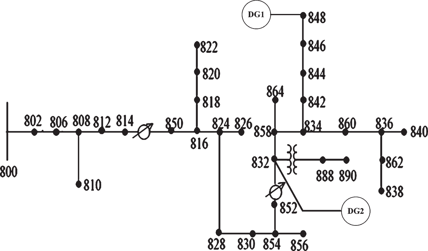
The test system corresponds to the IEEE standard of 34 nodes, with a nominal voltage of 24.9 kV. It is characterized by its large length, a section of 4.16 kV, unbalanced loads, a three-phase main feeder, multiple three-phase and single-phase side, point loads and capacitor banks [15, 16]. To consider the presence of DG sources in the EDS, two (2) of these sources are added in nodes 832 and 848 based on the considerations of [15], as shown in Fig. 1.
Fig.1
IEEE standard of 34 nodes with DG sources.
2.2Database
For the study of the circuit with sources of DG at the nodes indicated in Fig. 1, a penetration of 10% of these sources is considered as base. The different types of faults that can be presented in EDS are considered in the investigation with 6 different values of fault resistance between 5 and 30; in steps of 5, in total 1764 faults are generated.
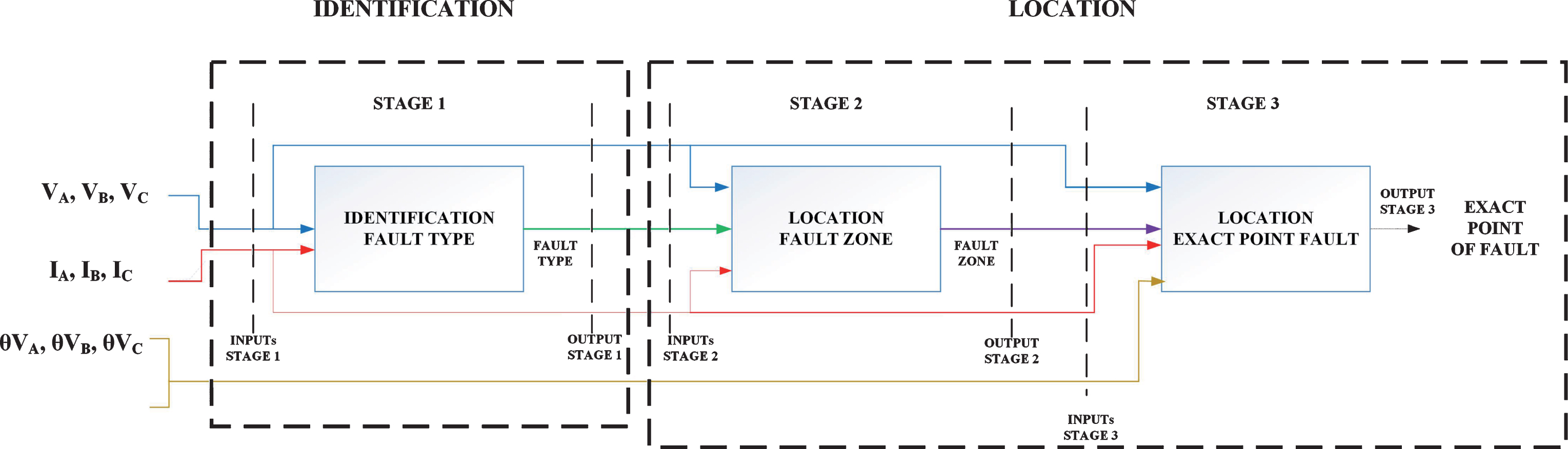
For each type of fault, the current and voltage values are obtained with their respective angles, measured in the substation and, additionally, in the node of the DG sources. From the database obtained, the schematic of fault diagnosis in EDS is designed. This scheme must be able to identify and locate the point of occurrence of the fault. To meet this need, 3 components are proposed for its design: identification of the type of fault, location of the fault zone, and the exact point of fault. Figure 2 shows the proposed scheme for the diagnosis of faults in EDS with DG.
Figure 2 shows that the purpose of the first block of the strategy is to identify the type of fault that occurs, which allows to activate the location block. The latter is divided into the location blocks of the fault zone and, finally, the location of the exact point of occurrence. Each of the components is detailed below.
Fig.2
Proposed scheme for the diagnosis of faults in EDS with DG.
2.3Identification of the type of fault
This block refers to identifying the type of fault that corresponds to each phase. The type is labeled with a number, which allows identification. The label for each type of fault is shown in Table 1. In this first block, the use of the Artificial Intelligence (AI) is proposed to treat the problem of the identification of the type of fault. Within AI techniques, SVM are the most used ones because of their better results compared to other techniques [17]. In this research, the SVM are used for this purpose. Measurements of voltage and current for each phase at the substation and DG sources are used as descriptors that provide fault event information. Different combinations of descriptors are obtained to train and test SVMs. Table 2 shows the combinations of descriptors used.
Table 1
Label to identify each type of fault
| Fault type | Phases involved | Label |
| Single phase | phase a – ground | 1 |
| phase b – ground | 2 | |
| phase c – ground | 3 | |
| phase-phase | phase a – phase b | 4 |
| phase b – phase c | 5 | |
| phase c – phase a | 6 | |
| phase-phase-ground | phase a – phase b – ground | 7 |
| phase b – phase c – ground | 8 | |
| phase c – phase a – ground | 9 | |
| Three-phase | phase a – phase b – phase c | 10 |
| Three-phase-ground | phase a – phase b – phase c - ground | 11 |
Table 2
Descriptors used to identify the type of fault with SVM
| Descriptor | Database used |
| Effective voltage values per phase | Va, Vb, Vc |
| Va1, Vb1, Vc1 | |
| Va2, Vb2, Vc2 | |
| Effective current values per phase | Ia, Ib, Ic |
| Ia1, Ib1, Ic1 | |
| Ia2, Ib2, Ic2 | |
| Effective voltage and current values per phase | Va, Vb, Vc Ia, Ib, Ic |
| Va1, Vb1, Vc1 | |
| Ia1, Ib1, Ic1 | |
| Va2, Vb2, Vc2 | |
| Ia2, Ib2, Ic2 |
Va, Vb, Vc: Effective voltage value per phase measured at the substation. Va1, Vb1, Vc1: Effective voltage value per phase measured at DG source located at node 848. Va2, Vb2, Vc2: Effective voltage value per phase measured at DG source located at node 832. Ia, Ib, Ic: Effective current value per phase measured at the substation. Ia1, Ib1, Ic1: Effective current value per phase measured at DG source located at node 848. Ia2, Ib2, Ic2: Effective current value per phase measured at DG source located at node 832.
For the SVM model the RBF kernel has been selected, which only needs to adjust its function parameter (γ) and error penalty factor (C). The RBF kernel does not correlate the samples in a higher dimensional space so that, unlike the linear kernel, it can handle the case when the relationship between the class labels and the attributes is not linear. In addition, the linear kernel is a special case of the RBF kernel [18]. The sigmoid kernel behaves like the RBF for certain parameters [19]. Another reason for selecting this function is the number of hyperparameters that influence the complexity of model selection. The polynomial kernel has more hyperparameters than the RBF. Finally, the RBF has fewer numerical difficulties [20].
The values of C and γ suitable for a given problem is unknown, so the selection of the model is made as a search of parameters to identify the best pair (C,γ) in a way that the classifier can accurately predict the unknown data (test data).
2.4Location of fault zone
This block refers to identifying the area within the EDS where the fault has occurred. The different zones are formed by the clustering of different nodes of the EDS to avoid problems of multiple fault estimation as the main problem of algorithmic methods [9]. Like the case of identification of the type of fault, each zone is labeled with a number that allows localization. Figure 3 shows the conformation of zones in the EDS.
The second block proposes the use of the AI for the location of the fault zone. Like the first block SVMs are used for the reasons described above. Effective voltage and current measurements for each phase obtained at the substation and DG sources provide the information to locate the fault zone. Different combinations of descriptors are obtained for training and testing the SVM, as indicated in Table 3.
Fig.3
Conformation of zones in the EDS.
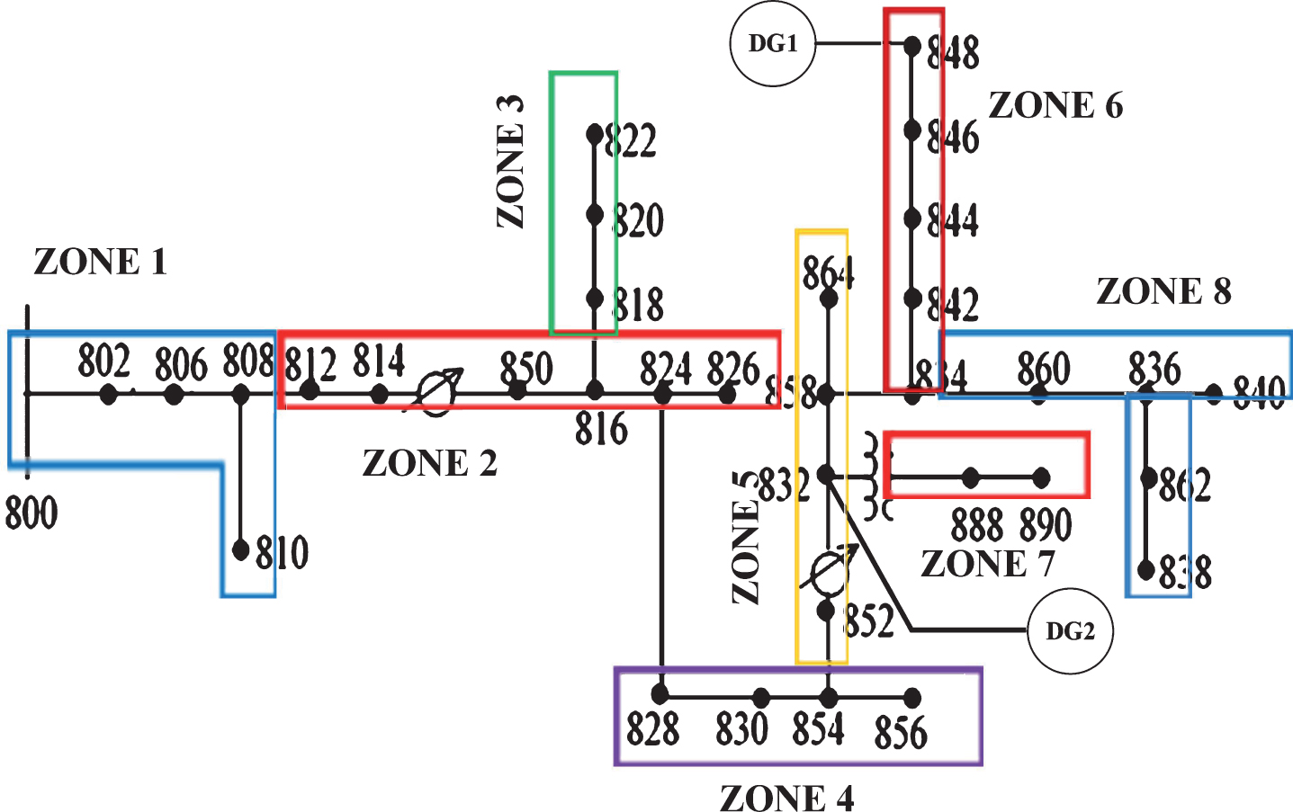
Table 3
Descriptors used to locate the fault zone with SVM
| Descriptor | Database used |
| Effective voltage values per phase | Va, Vb, Vc |
| Va, Vb, Vc | |
| Va1, Vb1, Vc1 | |
| Va2, Vb2, Vc2 | |
| Effective current values per phase | Ia, Ib, Ic |
| Ia, Ib, Ic | |
| Ia1, Ib1, Ic1 | |
| Ia2, Ib2, Ic2 | |
| Effective voltage and current values per phase | Va, Vb, Vc |
| Va1, Vb1, Vc1 | |
| Va2, Vb2, Vc2 | |
| Ia, Ib, Ic | |
| Ia1, Ib1, Ic1 | |
| Ia2, Ib2, Ic2 |
*The definition of the variables in the database is the same given in Table 2.
Similarly, for the SVM model, the RBF kernel has been selected which only requires that its parameter of the function (γ) and the error penalty factor (C) be adjusted.
2.5Locating exact point of fault
This block refers to knowing the exact point where the fault occurred within the EDS. It corresponds to the final stage and depends on the two (2) above, i.e., the identification of the type of fault and the location of the zone. To locate the exact point of fault, an algorithmic method based on the model of the electric network is proposed and whose inputs are the effective values of voltage and current with their respective angles, all measured in the substation and DG sources. Figure 4 shows an EDS in which the area where the fault occurred, located between the sources of GD and the substation, is known. For each EDS line, the exact model shown in Fig. 5 is used.
Fig.4
Fault located between substation and DG source in an EDS.
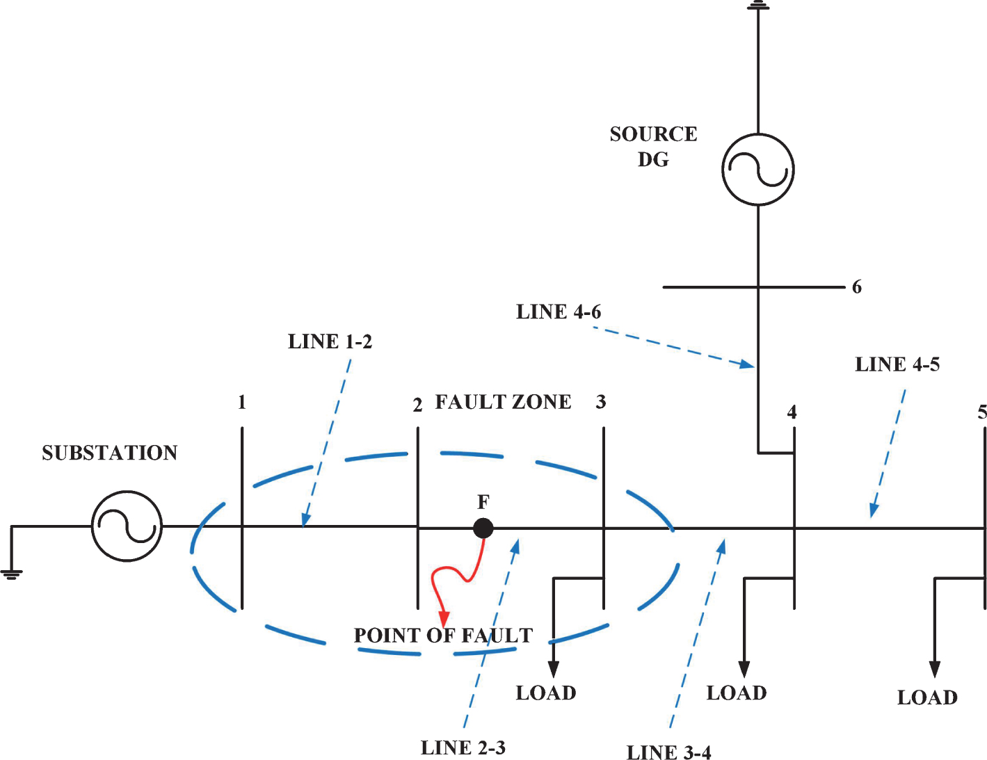
Fig.5
Line model considered in EDS.
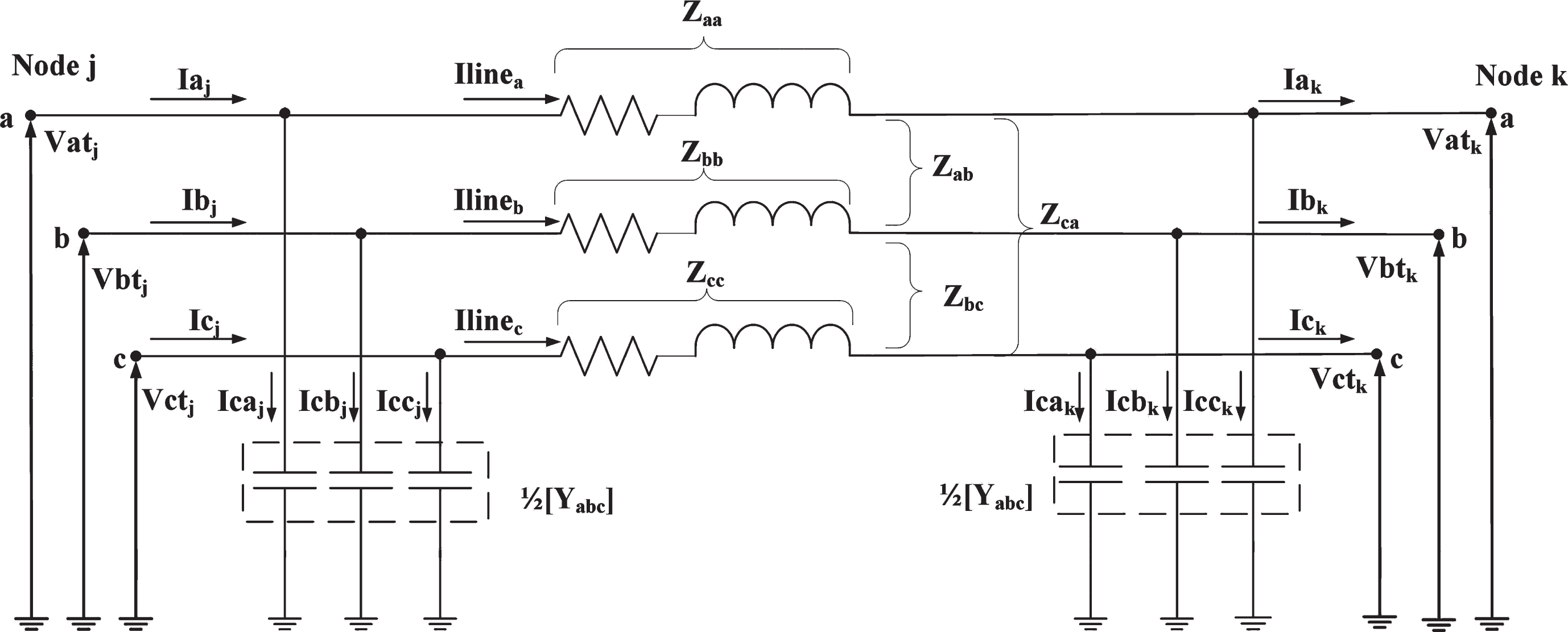
The voltage and current entering each of the nodes from the substation and/or DG sources to the fault zone can be determined by Equations (1 and 2), respectively. Additionally, the Equations (3 to 6) show their derivations.
(1)
(2)
(3)
(4)
(5)
(6)
where
1 [Vabcg] k: Phasor three-phase voltage at node k in V
2 [Iabc] k: Phasor three-phase current at node k in A
3 [Vabcg] j: Phasor three-phase voltage at node j in V
4 [Iabc] j: Phasor three-phase current at node j in A
5 [Zabc] Serie impedance matrix of the line segment jk in Ω
6 [Yabc]: Shunt admittance matrix of the line segment jk in S (Ω-1)
7 [U]: Identity matrix 3×3
The successive application of Equations (1 and 2) makes possible to estimate the voltages and currents at each node up to the fault zone. In each load node, the current must be updated by subtracting, from the current that enters the node, the demand for the connected load as indicated by Equation (7).
(7)
The [Iabc] kl represents the current coming from node k to node l, [Iabc] k corresponds to that which enters node k determined by Equation (2), and [Iload] k is demanded by the load connected at the node k. The location of the fault for each line segment within the zone is shown in Fig. 6.
Fig.6
Estimation of the distance for faults located between the substation and DG sources.
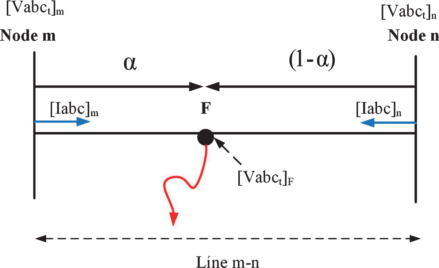
Using Kirchhoff’s Law of Tensions and Equation (1), we find Equations (8 and 9).
(8)
(9)
α: fault distance in per unit
Equations (8 and 9) in its real and imaginary components and organizing the terms gives Equations (10 and 11).
(10)
(11)
where:
(12)
(13)
(14)
(15)
(16)
(17)
The solution of Equations (10 and 11) is (18 and 19)
(18)
(19)
Equations (18 and 19) represent the fault distances in per unit for each phase and shows 2 possible solutions, due to their quadratic nature. According to the type of fault, Equations (18 and 19) are multiplied by a diagonal matrix of type of fault [ZF] which allows to consider the phase (s) involved in the fault. In this way, the fault distance will be given by Equation (20). Finally, the value of [ZF] is shown in Table 4 according to the type of fault.
Table 4
Fault type matrix
| Fault type | Phases involved | Matrix of type of fault |
| Single phase | A-g |
|
| B-g |
| |
| C-g |
| |
| phase-phase | A-B |
|
| B-C |
| |
| C-A |
| |
| phase-phase-ground | A-B-g |
|
| B-C-g |
| |
| C-A-g |
| |
| Three-phase | A-B-C |
|
| Three-phase-ground | A-B-C-g |
|
(20)
As the distance from the substation to the end node of the line segment is known, the actual distance from the substation will be known. Finally, the accuracy of the intelligent strategy is determined from the error, by means of Equation (21).
(21)
where:
1 d: Estimated distance of the fault (in km or in relative units in pu)
2 dexact: Exact distance of the fault (in km or in relative units in pu)
3 l: Total length of the line (in km or in relative units in pu)
3Results and discussion
3.1Identification of the type of fault
A mesh search is performed for several pairs of values (C, γ) by means of cross-validation and the one with the best accuracy is selected. The values considered for the parameters are shown in Table 5. Table 6 shows the best pairs of values (C, γ) for each database in the training stage.
Table 5
Values considered for the mesh search of (C, γ) by cross-validation
| Parameter | Values considered | Logarithmic values in base 2 |
| C | 2-10 to 2-20 | –10 to 20 |
| γ | 2-20 to 2-30 | –20 to 30 |
Table 6
Best pairs of values (C, γ) for each database
| Database | C | γ | Accuracy in training (%) |
| Va, Vb, Vc | 262.144 | 1 | 97,88 |
| Va1, Vb1, Vc1 | 16.384 | 0,0625 | 99,33 |
| Va2, Vb2, Vc2 | 262.144 | 0,0625 | 99,46 |
| Ia, Ib, Ic | 262.144 | 16 | 98,79 |
| Ia1, Ib1, Ic1 | 16.384 | 16 | 99,82 |
| Ia2, Ib2, Ic2 | 16.384 | 16 | 99,82 |
| Va, Vb, Vc | 16.384 | 0,0625 | 100 |
| Ia, Ib, Ic | |||
| Va1, Vb1, Vc1 | 4 | 16 | 100 |
| Ia1, Ib1, Ic1 | |||
| Va2, Vb2, Vc2 | 4 | 16 | 100 |
| Ia2, Ib2, Ic2 |
Table 7
Accuracy in the test stage of the SVM for the identification of the type of fault
| Database | Amount | Amount of | Accuracy in |
| of test | data correctly | the test | |
| data | classified | stage (%) | |
| Va, Vb, Vc | 110 | 110 | 100 |
| Va1, Vb1, Vc1 | 110 | 110 | 100 |
| Va2, Vb2, Vc2 | 110 | 110 | 100 |
| Ia, Ib, Ic | 110 | 105 | 95,45 |
| Ia1, Ib1, Ic1 | 110 | 107 | 97,27 |
| Ia2, Ib2, Ic2 | 110 | 110 | 100 |
| Va, Vb, Vc Ia, Ib, Ic | 110 | 110 | 100 |
| Va1, Vb1, Vc1 | 110 | 110 | 100 |
| Ia1, Ib1, Ic1 | |||
| Va2, Vb2, Vc2 | 110 | 110 | 100 |
| Ia2, Ib2, Ic2 |
From Table 6, the accuracy obtained by the SVMs in the training stage can be appreciated through cross-validation with mesh search. The highest accuracy corresponds to the databases composed of the effective values of voltage and current measured per phase in the substation. In another sense, the lower accuracy corresponds to the databases composed of a descriptor, that is, or only the measurements of the effective values of voltage or current, all these in the substation and in the DG sources.
To evaluate the performance of the SVM in the identification of the type of fault against unknown data (test data), the test stage is carried out with ten data for each type of fault, which were not used during the training stage. The total amount of test data for the 11 fault types was 110 for each database used, these were randomly selected. Table 7 shows the accuracy in the test stage of the SVMs for the identification of the type of fault in the EDS.
The accuracy in the test stage is defined as shown in Equation (22):
(22)
3.2Location of fault zone
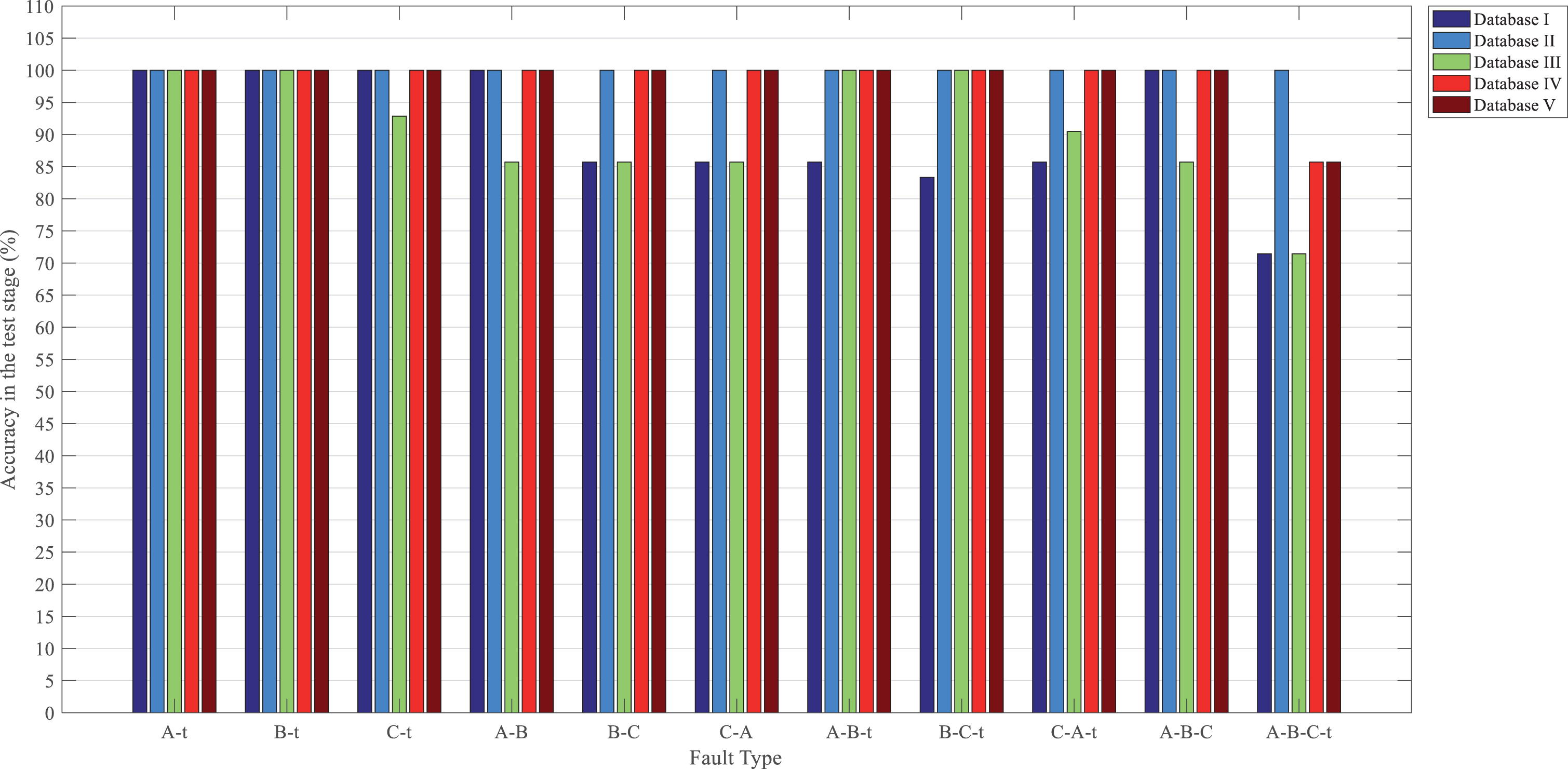
To evaluate the performance of the SVMs in the location of the fault zone against unknown data (test data), the test stage is carried out with 468 data in total, for the different types of fault, which were not used during the training stage. Figure 7 shows the results obtained from the SVMs for the location of the fault zone in the EDS. From Fig. 7 it is observed that the database that has the perfect accuracy in the test stage is II, which is made up of the effective voltage values measured in the substation and in the DG sources.
Fig.7
Results of the location of fault zone in the EDS. Database I: Va, Vb, Vc; Database II: Va, Vb, Vc; Va1, Vb1, Vc1; Va2, Vb2, Vc2; Database III: Ia, Ib, Ic; Database IV: Ia, Ib, Ic; Ia1, Ib1, Ic1; Ia2, Ib2, Ic2; Database V: Va, Vb, Vc; Va1, Vb1, Vc1; Va2, Vb2, Vc2; Ia, Ib, Ic; Ia1, Ib1, Ic1; Ia2, Ib2, Ic2.
3.3Location exact point of fault
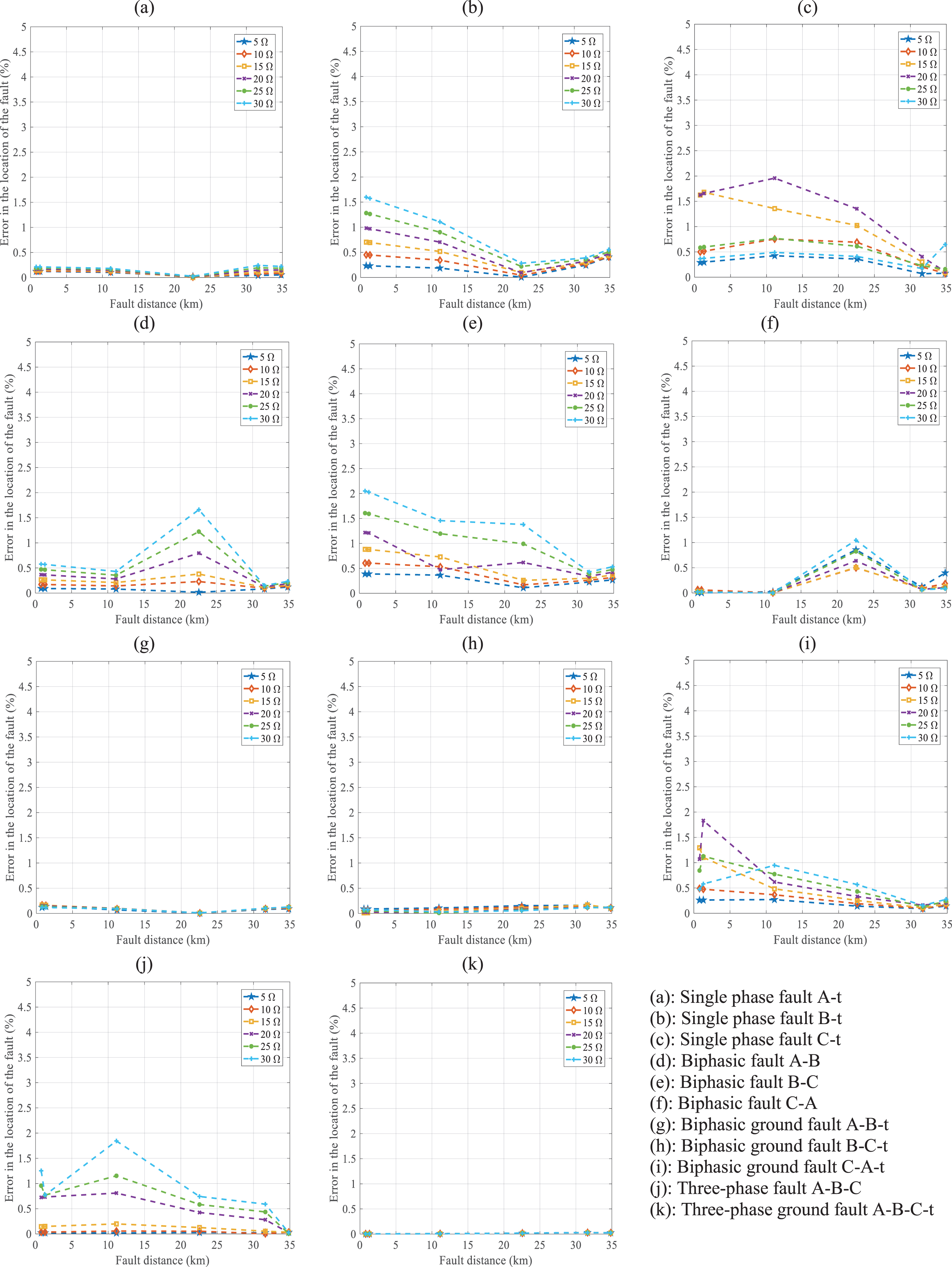
Figure 8 shows the errors in the location of the fault point for the different types of fault, varying the fault resistance and the distance measured from the substation. The accuracy depends on the measurement of the error determined by means of Equation (21). Figure 8 shows variations of the percentage error in the location of the fault point, which range from 0 to 2%. Single-phase faults have errors that do not reach 2%, biphasic faults maximum of 1.6%, biphasic faults to ground of up to 1.8%, three-phase faults of up to 1.8%, and three-phase faults to ground present the lowest error of all with a maximum value of 0.03%. Regarding to the distance, a similar error pattern is shown in each type of fault when the resistance varies, however, when increasing the distance of occurrence, the error varies according to the type of fault. This behavior can be explained due to the presented scheme which, as a previous stage to finding the point of fault, locates the fault zone; this allows the distance measured from the substation to the initial node of the fault zone to be known, with which the calculation of the error is made from the point already known. The use of SVMs as AI tools for the identification of the type of fault and the location of the zone presents better results than those found in [11] and also considers variation of the fault resistance, variation of the penetration of DG and variation of the load, cases that have not yet been reported. The results shown in Fig. 8 have similarity to those reported in [21] regarding the type of fault and fault resistance, however, the errors found by the proposed scheme when varying the fault resistance are less than indicated in [21]. The conformation of the scheme proposed by stages allows that the activation of the block of location of the point of fault is with the knowledge of the type and of the zone of fault, what avoids the consideration of different models for each type of fault and its iterative use until its convergence as shown in [6, 15]. The solution given by the proposed scheme is unique and avoids the consideration of different possible solutions as reported in [15], nor does it depend on the response of the protection devices that are installed along the feeder as it considers [22]. Finally, the scheme consisting of integrated methods for locating faults in EDS with the presence of DG has not yet been reported in the reviews carried out [23–28]. One of the novelties of the proposed strategy is that it avoids the estimation of the section of the line where the fault is found through iterative methods that establish a convergence criterion as shown in [15]. On the other hand, when knowing the fault zone, the location of the exact point of failure is faster about computational times.
Fig.8
Errors in location of the point of fault.
4Conclusions
A scheme for the location of faults in EDS with GD is presented. A base composed of 1764 fault data is generated that considers the 11 different types of faults that can occur in a EDS, for 6 different values of fault resistance from 5 to 30 Ohm, in steps of 5 Ohm. The scheme is integrated using artificial intelligence and mathematical algorithms based on the system model, and it is proposed by means of 3 stages: Identification of the type of fault, location of the fault zone, and location of the exact point of fault.
The results show a perfect identification of the type of fault and the fault zone with maximum errors of 2% in the location of the point of fault. The location of the exact point of fault maintains errors lower than 2%, which demonstrates the performance of the proposed scheme.
The proposed strategy for fault location considers actual operating conditions in electrical distribution systems such as unbalanced conditions, single-phase branches, unbalanced loads, among others. In addition, the mathematical model for the exact location of the point of failure considers the presence of capacitive effects in the distribution lines. Additionally, the presence of distributed generation sources makes the proposed strategy robust in practical applications.
References
[1] | Kezunovic M. , Smart fault location for smart grids, IEEE Transactions on Smart Grid 2: (1) ((2011) ), 11–22. |
[2] | Pérez R. and Vásquez C. , Fault Location in Distribution Systems with Distributed Generation Using Support Vector Machines and Smart Meters, IEEE Ecuador Technical Chapters Meeting (ETCM), (2016) , pp. 1–6. |
[3] | Menchafou Y. , Markhi H. , Zahri M. and Habibi M. , Impact of distributed generation integration in electric power distribution systems on fault location methods, 3rd International Renewable and Sustainable Energy Conference (IRSEC), no. 1998, (2015) . |
[4] | Fazanehrafat A. , Javadian S. , Bathaee S. and Haghifam M. , Maintaining the recloser-fuse coordination in distribution systems in presence of DG by determining DG’s size, IET 9th International Conference on Developments in Power Systems Protection (DPSP 2008), (2008) , pp. 132–137. |
[5] | José B. , Cavalcante P. , Trindade F. and Almeida M. , Analysis of Distance Based Fault Location Methods for Smart Grids with Distributed Generation, 2013 4th IEEE PES Innovative Smart Grid Technologies Europe (ISGT Europe), (2013) , pp. 1–6. |
[6] | Orozco C. , Mora J. and Pérez S. , Método de localización de fallas basado en impedancia aparente para sistemas de distribución con generación distribuida, Ingeniare Revista Chilena de Ingenier&a 23: (3) ((2015) ), 348–360. |
[7] | Mora J. , Meléndez J. and Carrillo G. , Comparison of impedance based fault location methods for power distribution systems, Electric Power Systems Research 78: (4) ((2008) ), 657–666. |
[8] | Awalin L. , Mokhlis H. and Bakar A. , Recent developments in fault location methods for distribution networks, Przeglad Elektrotechniczny 12: ((2012) ), 206–212. |
[9] | Mirzaei M. , Kadir M. , Moazami E. and Hizam H. , Review of fault location methods for distribution power system, Australian Journal of Basic and Applied Sciences 3: (3) ((2009) ), 2670–2676. |
[10] | Javadian S. and Massaeli M. , A fault location method in distribution networks including DG, Indian Journal of Science and Technology 4: (11) ((2011) ), 1446–1451. |
[11] | Agrawal R. and Thukaram D. , Identification of fault location in power distribution system with distributed generation using support vector machines, 2013 IEEE PES Innovative Smart Grid Technologies Conference (ISGT), (2013) , pp. 1–6. |
[12] | Ratnadeep K. , Bhosale Y. and Kulkarni S. , Fault level analysis of power distribution system, 2013 International Conference on Energy Efficient Technologies for Sustainability, (2013) , pp. 1001–1005. |
[13] | Prakash M. , Pradhan S. and Roy S. , Soft Computing Techniques for Fault Detection in Power Distribution Systems: A Review, Green Computing Communication and Electrical Engineering (ICGCCEE), 2014 International Conference on, (2014) , pp. 1–6. |
[14] | Mohammadi P. , Kishyky E. , Akher A. and Salam A. , The impacts of distributed generation on fault detection and voltage profile in power distribution networks, International Power Modulator and High Voltage Conference (IPMHVC), (2014) , pp. 191–196. |
[15] | Alwash S. , Ramachandaramurthy V. and Mithulananthan N. , Fault-location scheme for power distribution system with distributed generation, IEEE Transactions on Power Delivery 30: ((2015) ), 1187–1195. |
[16] | IEEE Power Engineering Society, “IEEE 34 Node Test Feeder,”, (2010) . |
[17] | Gururajapathy S. , Mokhlis H. and Illias H. , Fault location and detection techniques in power distribution systems with distributed generation: A review, Renewable and Sustainable Energy Reviews 74: (February 2016) ((2017) ), 949–958. |
[18] | Keerthi S. and Lin C. , Asymptotic behaviors of support vector machines with Gaussian kernel, Neural Computation 15: (7) ((2003) ), 1667–89. |
[19] | Lin H. and Lin C. , A study on sigmoid kernels for SVM and the training of non-PSD kernels by SMO-type methods, Neural Computation 2: ((2003) ), 1–32. |
[20] | Hsu C. , Chang C. and Lin C. , A practical guide to support vector classification, BJU international 101: (1) ((2008) ), 1396–400. |
[21] | Jamali S. and Talavat V. , Accurate fault location method in distribution networks containing distributed generations, Iranian Journal of Electrical and Computer Engineering 10: (1) ((2011) ), 27–33. |
[22] | Brahma S. , Fault location in power distribution system with penetration of distributed generation, IEEE Transactions on Power Delivery 26: (3) ((2011) ), 1545–1553. |
[23] | Dashti R. and Sadeh J. , Fault section estimation in power distribution network using impedance-based fault distance calculation and frequency spectrum analysis, IET Generation, Transmission & Distribution 8: (8) ((2014) ), 1406–1417. |
[24] | Gazzana D. , Ferreira G. , Bretas A. , Bettiol A. , Carniato A. , Passos L. , Ferreira A. and Silva J. , An integrated technique for fault location and section identification in distribution systems, Electric Power Systems Research 115: ((2014) ), 65–73. |
[25] | Mora J. , Barrera V. and Carrillo G. , Fault location in power distribution systems using a learning algorithm for multivariable data analysis, IEEE Transactions on Power Delivery 22: (3) ((2007) ), 1715–1721. |
[26] | Salim R. , de Oliveira K. FilomenaA. ResenerM. and BretasA. Hybrid fault diagnosis scheme implementation for power distribution systems automation, IEEE Transactions on Power Delivery 23: (4) ((2008) ), 1846–1856. |
[27] | Trindade F. and Freitas W. , Low voltage zones to support fault location in distribution systems with smart meters, IEEE Transactions on Smart Grid pp: (99) ((2016) ), 1–10. |
[28] | Pérez R. , Inga E. , Aguila A. , Vásquez C. , Lima L. , Viloria A. and Henry M. , Fault diagnosis on electrical distribution systems based on fuzzy logic, Advances in Swarm Intelligence ICSI 2018 Lecture Notes in Computer Science 10942: ((2018) ), 174–185. |


