
Prediction of critical safety factor of slopes using multiple regression and neural network
Abstract
The estimation of slope stability is an engineering problem that involves many parameters. The impact of these parameters on the stability of slopes can be understood by the use of computational tools like regression analysis, neural networks, etc. These computational tools are highly sophisticated modelling techniques which are capable of modelling very complex functions. They act as a powerful tool for modelling, especially when the relationships between the underlying data is unknown. It can identify and understand the correlated patterns present between the input data sets and corresponding target values. In this paper, the input data for the three dimensional slope stability estimation includes the geotechnical and geometrical input parameters and the 3-D critical safety factor (Fcs) as the output data. On successful completion of the model, the performance of the same is measured and the results are compared to those obtained by means of standard analytical methods. The results showed that the predicted values are very close to the analytical values and provide good correlation between the input variables.
1Introduction
With the introduction of multiple linear regression (MLR) and artificial neural network (ANN), engineers and researchers from a variety of disciplines are encouraging researches using these applications. The growing interest among the researchers is due to the excellent performance provided by these learning machines in pattern recognition and modelling of non-linear multivariate dynamic systems. The accurate estimation of the soil stabilization is a very challenging task for the geotechnical engineers due to the intricacy and difficulty in determining the geotechnical input data parameters. The slope stability analysis must be carried out by considering the various important parameters like site sub-surface conditions, ground behaviour, applied loads, etc. It is due to its practical importance that slope stability analysis has drawn the attention of many investigators. This paper investigates the validity of utilizing MLR and ANN in the physical problem of three dimensional slope stability prediction. Although the slope stability prediction is a very challenging task yet it has developed its existence to a great extent in the last two decades. Many researchers from the geotechnical background are constantly working to find new prediction models for determining the two dimensional slope stability. But very few research articles are available based on the prediction analysis of three dimensional slope stability. Chang [1] based on the 1988 Kettleman Hills landfill failure mechanism developed a 3D slope stability prediction model. The prediction model found to be very accurate in calculating the three dimensional slope stability involving a translational type of failure along a pre-existing slip surface but the model is found to be not fully applicable for dense sands or over consolidated materials under drained conditions. Sakellariou and Ferentinou [2] used ANN to predict the two dimensional slope stability of slopes for circular failure and wedge failure mechanism and found that the predicted results are very close to the analytical results. Kayesa [3] predicted the slope failure of Letlhakane mine using Geomos slope monitoring system which contributed a lot in avoiding potentially fatal injury and damage to mining equipments. Davis and Keller [4] used fuzzy sets and Monte Carlo Simulation technique for predicting the two dimensional slope stability analysis and found that the input parameters are having good correlation with the output parameters. The use of evolutionary polynomial regression (EPR) technique for predicting the stability of soil and rock by Ahangar-Asr et al. [5] is found to be very effective and robust in slope behaviour modeling. Mohammad et al. [6] used the concept of fuzzy logic system and multiple linear regression (MLR) technique for prediction the two dimensional slope stability and found that the fuzzy logic model has higher degree of precision in predicting the slope stability. Erzin and Cetin [7] developed another prediction model using ANN and multiple regression (MR) for estimating the FOS of an artificial slope subjected to earthquake forces. The results inferred that ANN model has higher prediction performance than the MR model. Chakraborty and Goswami [8, 9] used statistical method for predicting the two dimensional slope stability analysis and found that the regression coefficient is found to be 94.9% bearing a very close relationship between the predictors. They continued their research work and in the same year they developed another prediction model for predicting the slope stability by using ANN. They found a very close relationship between the predictors with R value of 0.98 and RMSE value of 0.06.
The use of stability charts by some of the researchers for predicting the three dimensional slope stability analysis was found to be very helpful. Michalowski [10] prepared stability charts using three dimensional failure mechanism for predicting the factor of safety. These charts are found to be very helpful in calculating the factor of safety as it does not require any iteration methods. Again Michalowski and Martel [11] developed some modified form of stability charts which can be carried out to seismic shaking. These modified charts are found to be very helpful in cases of excavation slopes. Gao et al. [12] used kinematically admissible rotational failure mechanism for developing stability charts for three dimensional homogenous slopes under both static and pseudostatic seismic loading conditions. These charts not only provides closer estimates of FOS but also it identifies the type of critical failure mechanism. Lim et al. [13] produce a set of stability charts for three dimensional slopes for a specific case in which frictional fill materials are placed on purely cohesive clay. The charts are found to be convenient tools for geotechnical engineers during design in practice.
2Multiple linear regression (MLR)
Regression analysis is a statistical tool for predicting the nature of relationship among different variables. According to Yilmaz and Yuksek [14], the general purpose of MLR is to learn more about the relationship between several independent or predictor variables and a dependent or criterion variable. This technique is widely used in predicting slope failures and landslides [15, 16]. The general equation for multiple regression is
(1)
Where Y = Dependent Variable
1 x1, x2, x3, ..., xn = Independent Variable
2 b1, b2, b3, ..., bn = Regression co-efficient
3 a = constant
4 ∈= error
In this equation, the regression coefficients represent the independent contributions of each independent variable to the prediction of the dependent variable. The regression line expresses the best prediction of the dependent variable (Y), given the independent variables (X). However, the nature is rarely perfectly predictable, and hence there is always a substantial variation of the observed points around the fitted regression line. The deviation of a particular point from the regression line is called the residual value. R-Square, also known as the Coefficient of determination is used to evaluate model fit which is given by 1 minus the ratio of residual variability. Smith [17] suggested the following guide for values of |R| (Square root of R-square) between 0.0 and 1.0:
|R|≥0.8 strong correlation exists between two sets of variables;
0.2< |R|<0.8 correlation exists between the two sets of variables; and
|R|≤0.2 weak correlation exists between the two sets of variables.
3Artificial neural network (ANN)
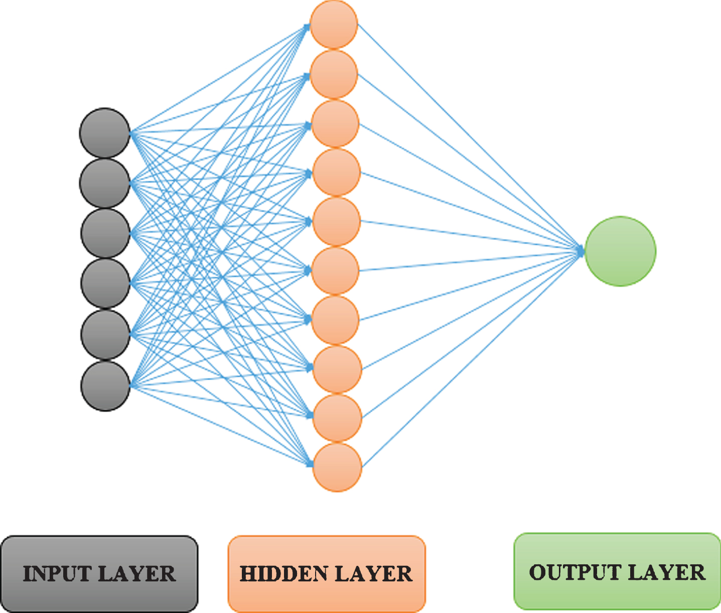
An Artificial Neural Network (ANN) is a mathematical model which works similar to the neurons present in the brain. It act as a powerful tool for modelling, specifically when the relationships between the underlying data is unknown. It can identify and understand the correlated patterns present between the input data sets and corresponding target values. ANNs are thus very helpful in modeling the complex nature of the most geotechnical materials which, by their very nature exhibit extreme variability. The schematic diagram of a neural network is shown in Fig. 1.
Fig.1
Schematic diagram of a neural network.
3.1Neuron model and network architecture
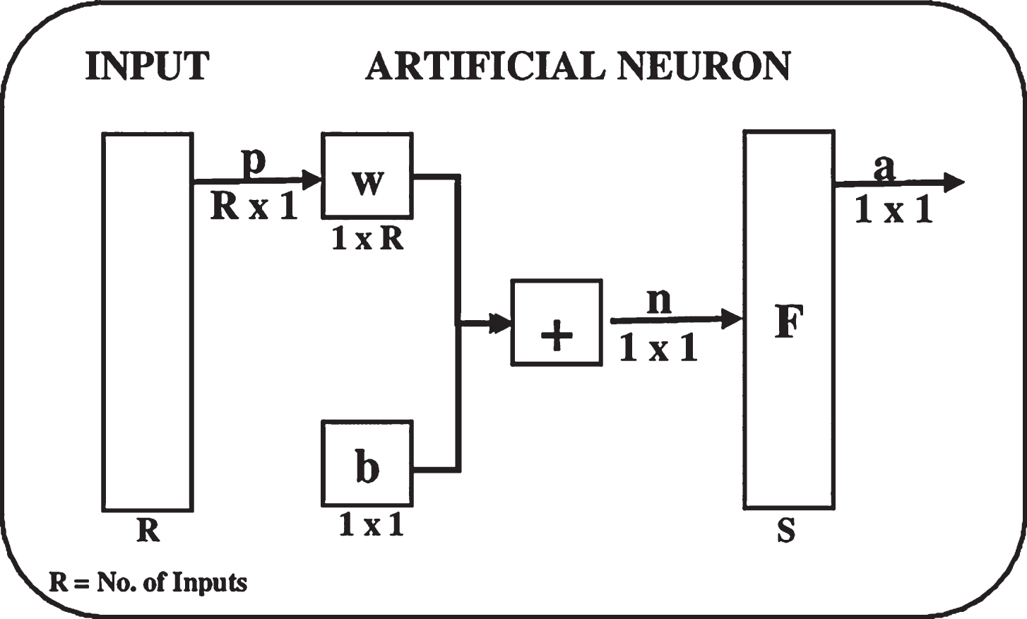
The neuron model and the network architecture enlightens how a network transmutes its input into an output. The way a network computes its output must be understood before training methods for the network can be explained. Let us consider a single artificial neuron with R inputs as shown in the Fig. 2. Here, the input vector p (a column vector, R x 1) is shown by a vertical bar on the left. These inputs go to the row vector w of size 1 x R. The net input n given by the sum of bias b and the product w x p is passed to the transfer function F to obtain the neuron’s output.
Fig.2
Artificial neuron model.
Depending upon the nature of the problem, the transfer function F can be linear or sigmoidal. The sigmoidal transfer function is commonly used in multiple-layer networks [18, 19]. In a multilayer network shown in Fig. 3, the outputs of the intermediate layer are the inputs to the following layer. Thus, layer 2 can be analyzed as a single layer network with R = S1 inputs, S = S2 neurons, weight matrix w = (S1×S2). The input to the layer 2 is p = a1 and the output is a = a2.
Fig.3
Multi-layer feed-forward network.
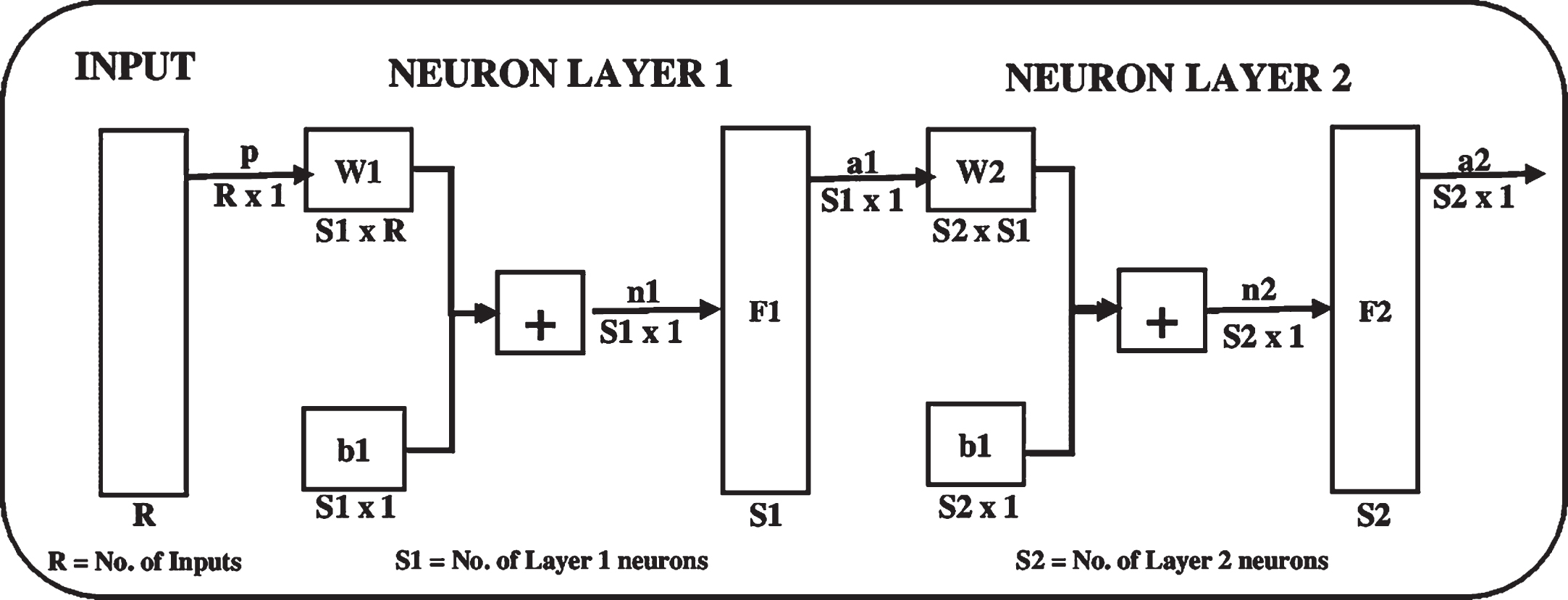
The layers of a multi-layer network plays a different role. A layer that produces the network output is called an output layer while all other layers in the network are called the hidden layers. The two layer network shown above has one output layer and one hidden layer. Multi-layer networks are much powerful compared to single layer networks as they are capable of using the combination of sigmoidal and/or linear transfer function.
3.2Training and validation of the model
The process of optimizing the connection weights is known as training. The most widely used training method for multi-layer neural feed-forward networks is Levenberg-Marquardt back-propagation algorithm [20]. The stopping criteria is considered to be the most important criteria and are used to stop the training process. They determine whether the model has been trained optimally [21]. Training can be stopped after the presentation of a fixed number of training records, when the training error reaches a sufficiently small value, or when no or slight changes in the training error occur. To avoid over fitting of the model, cross validation technique is used [22, 23]. The cross-validation technique requires the data to be divided into training set, testing set and validation set. The objective of training is to find the set of weights between the neurons that determine the global minimum of error function. The main function of the testing set is to evaluate the generalization ability of a trained network and the validation set performs the final check of the trained network. Training is stopped when the error of the testing set starts to increase. Once the training phase of the model is successfully completed, the performance of the trained model should be validated. The validation phase of the model is performed to check the generalization ability of the trained model within the limits set by the training data in a robust fashion, rather than simply memorizing the input-output relationships that are contained in the training data. The best approach to validate the trained model is to test the performance of the same on an independent data set, which has not been used as part of the model building process. If such performance is adequate, the model is deemed to be able to generalize and is considered to be robust. The coefficient of correlation, R, the root mean squared error, RMSE, and the mean absolute error, MAE, are the main criteria that are often used to evaluate the prediction performance of ANN models.
4Methodology
In this research, 3500 artificial slopes having different geometrical and geotechnical parameters are analyzed using finite element method to determine the 3-D critical safety factor of slopes. The analytical values are used to develop the prediction models using MLR and ANN. In the proposed models for predicting 3D critical safety factor, several important parameters including, height of the slope (H), cohesion (c), angle of internal friction (φ), slope inclination (β), unit weight of soil (γ) and dimensionless parameter (m) are used as input parameters whereas the 3-D critical safety factor (Fcs) is used as the output parameter. The dimensionless parameter, ‘m’ is defined as the ratio between the water table depth (dw) and the width of the slope (B). The water table depth (dw) is an alternative quantity for the active pore pressure. The pore pressure at a depth, z, below the surface is given by:
(2)
The MLR model for predicting the critical safety factor is developed using Microsoft Excel 2013.
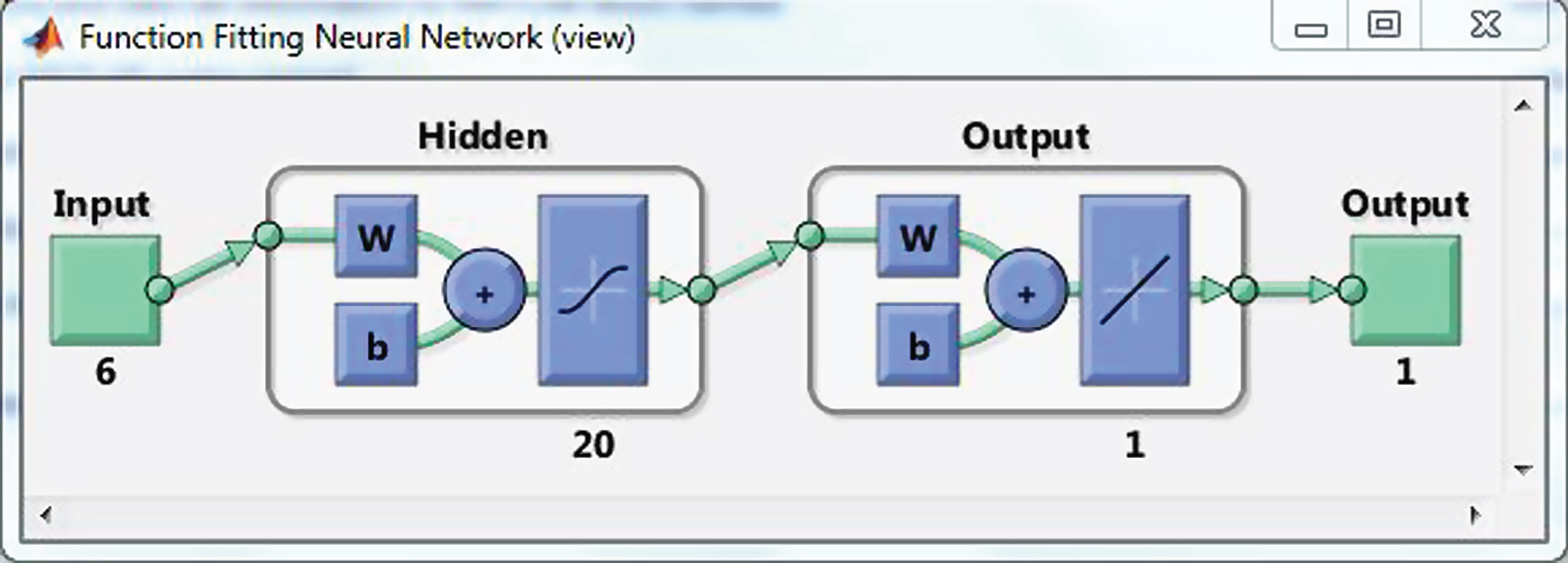
The ANN model is prepared in Matlab version R2011a. Here, multi-layer feed-forward network having 20 neurons in hidden layer and 1 neuron in output layer is used for developing the prediction model which is shown in Fig. 4.
Fig.4
Neural network showing hidden neurons.
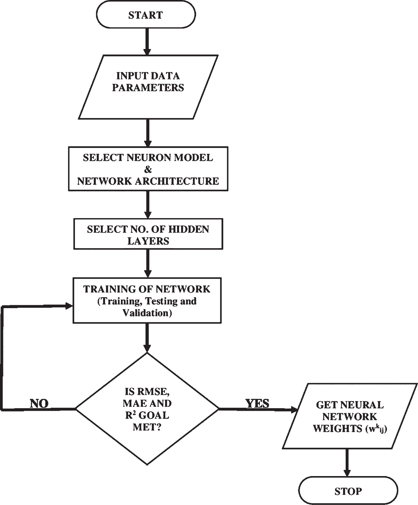
For the cross validation technique, the whole data set (3500) used for the development of the prediction model is divided into three distinct sets i.e. training set (80% data), testing set (10% data) and validation set (10% data). The network is trained up using Levenberg-Marquardt back propagation till the training error reaches a sufficiently small value, or when no or slight changes in the training error occur. In other words, training is stopped when the regression coefficient R of all the three sets, i.e., training, testing and validation approaches close to unity. The flow chart for determination of neural network weights (wkij) is shown in Fig. 5.
Fig.5
Flowchart showing determination of neural network weights.
5Results and discussion
The 3-D Fcs values obtained by FEM are used to develop MLR and ANN models to obtain the prediction formula for the determination of critical safety factor of slope. The summary of the results obtained by both the models is given below:
5.1Multiple linear regression (MLR)
The summary of MLR for 3500 artificial slope cases is shown in Table 1. From the Table below it has been found that the “p” value for all the stability parameters is less than 0.05 (having 95% confidence level). Moreover, the value of both R-square and adjusted R-square has been found to be 0.884.
Table 1
Summary of MLR for 3500 artificial slope cases
| SUMMARY OUTPUT | ||||
| Regression Statistics | ||||
| Multiple R | 0.940 | |||
| R Square | 0.884 | |||
| Adjusted R Square | 0.884 | |||
| Standard error | 0.171 | |||
| Observations | 3500 | |||
| Stability parameters | Coefficients | Standard Error | t Stat | P-value |
| Intercept | 2.551 | 0.047 | 53.736 | 0 |
| H | –0.074 | 0.001 | –83.592 | 0 |
| c | 0.023 | 0.000 | 115.914 | 0 |
| φ | 0.034 | 0.000 | 100.929 | 0 |
| β | –0.018 | 0.000 | –81.951 | 0 |
| γ | –0.036 | 0.002 | –15.448 | 0 |
| m | –0.195 | 0.014 | –14.219 | 0 |
5.2Artificial neural network (ANN)
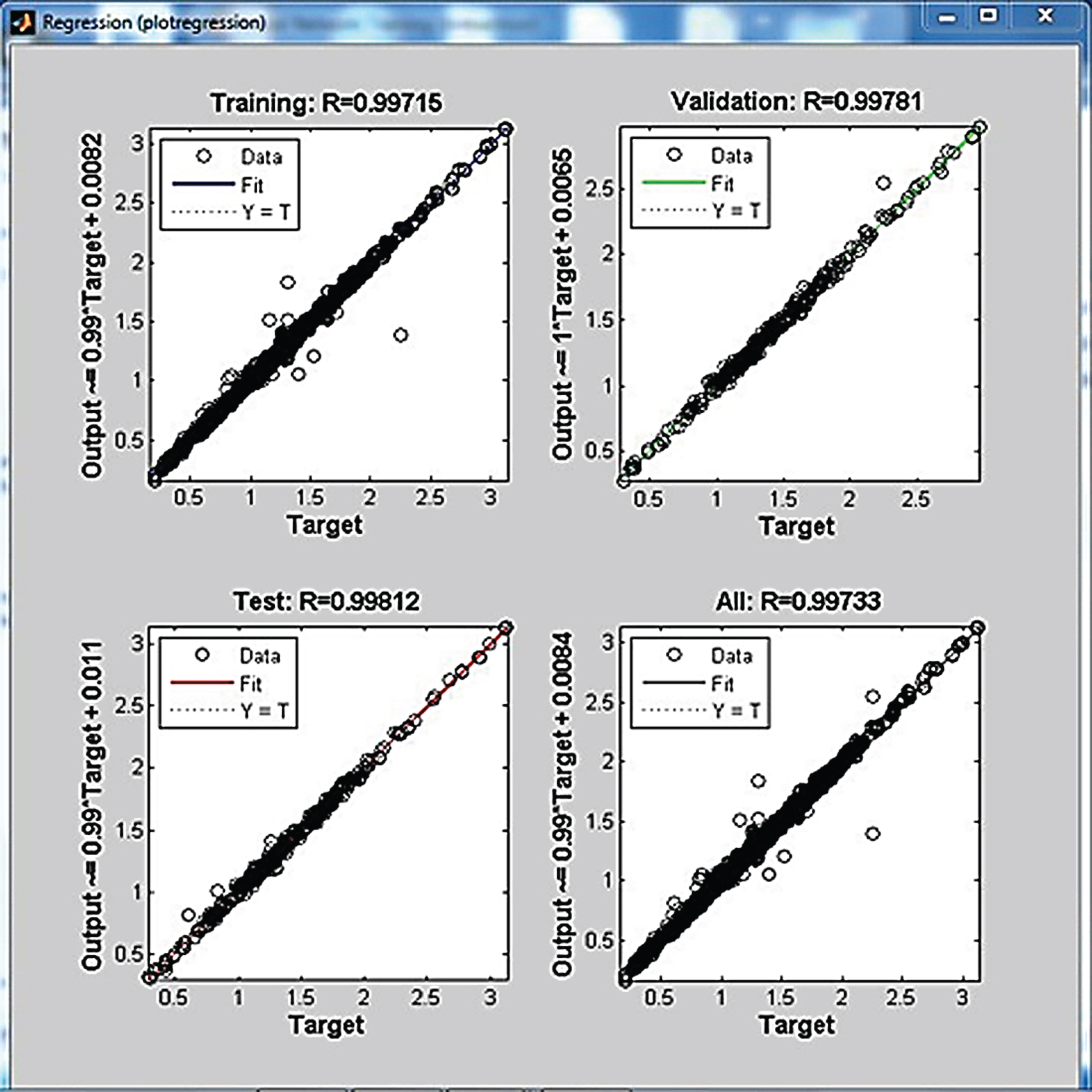
The regression plot showing the value of R for training, testing and validation is shown in Fig. 6. From the regression plot, it has been found that the value of R to be 0.99 bearing a close relationship between the input variables.
Fig.6
Regression plot of the network model.
The performance of the predicted models are checked by examining the results by making predictions against case records which are not used during training and testing. The validation performance of the network model is shown in Fig. 7. 10 vulnerable slope cases around Guwahati, Assam, India having different latitude and longitude are selected. A preliminary site investigation is done to get an idea about the geology of the site. The investigation report delivers that under favorable conditions of temperature, pressure, rainfall and drainage, intense weathering of rocks of granitic origin leads to formation of residual soils. Rocks found in landslide areas of Guwahati are mostly of igneous and metamorphic origin. Granite gneiss, which is a major country rock of the area shows varying degree of weathering at various landslide areas. At Hengerabari and Sunsali landslide area, it is observed at a highly weathered stage. At Dhirenpara and Kharguli landslide area it is found to be moderately weathered. Along with the granite gneiss, porphyritic granite are also found in some of the landslide areas of Guwahati. In addition to this, micaceous soils have also been encountered in some parts of the landslide areas of Sunsali. A carefully planned subsoil investigation consisting of drilling of exploratory borehole at the predefined location is carried out using auger and wash boring process. Soil samples are collected and laboratory triaxial tests are conducted to determine the geotechnical (shear) parameters of the soil. Total station survey has been conducted to plot the contour map of the slope using Teraplot LT. From the contour map different geometrical parameters are determined. These geometrical and geotechnical parameters are used to determine the 3-D critical safety factor of slopes and a comparison is made using the results of analytical, MLR and ANN as shown in Table 2. It is evident from Fig. 8 that the prediction model by ANN is found to have higher correlation of over 98% compared to that obtained by MLR having only 93%. Hence, it can be said that ANN can give higher correlation compared to the other prediction models.
Fig.7
MSE plot of the network model.
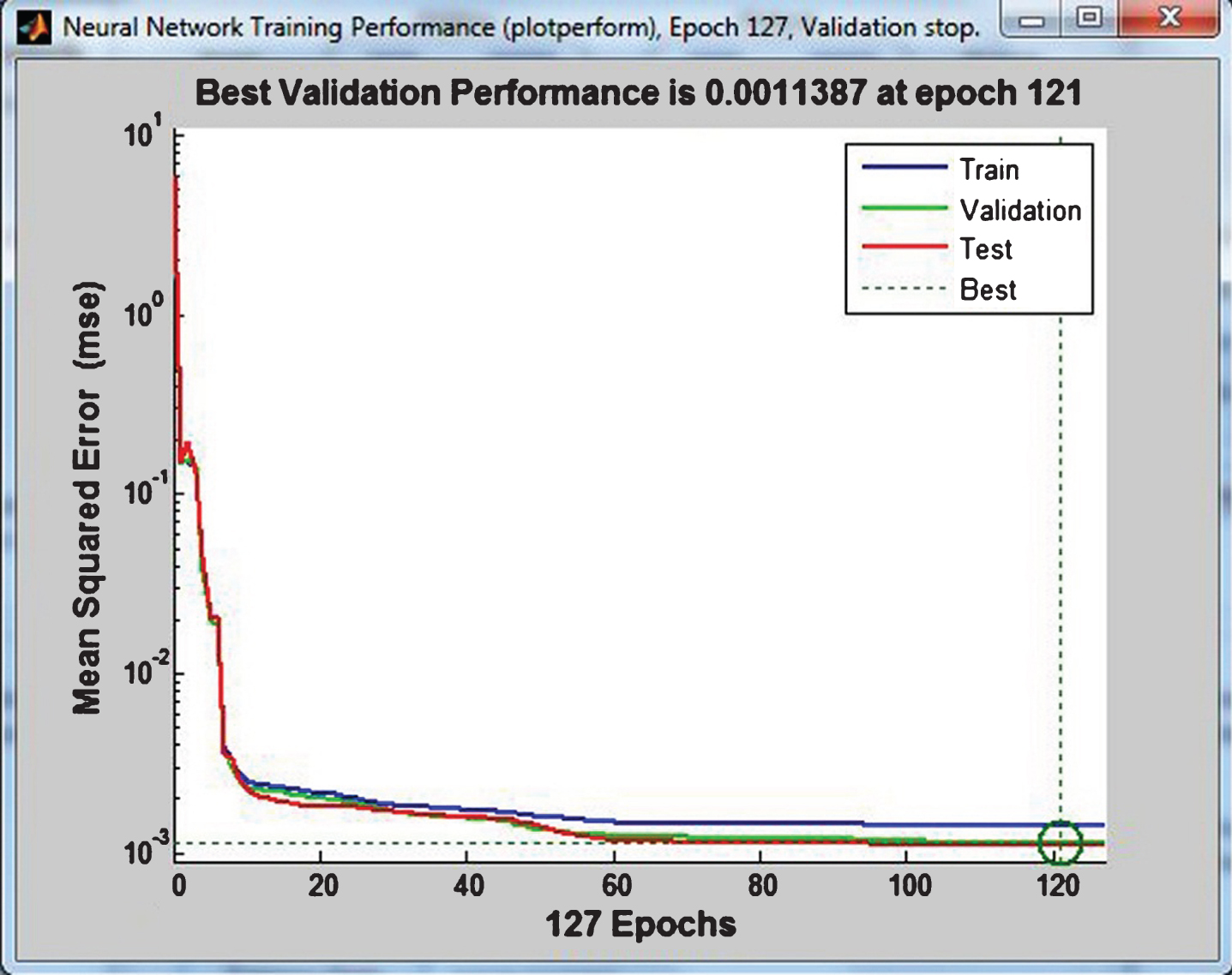
Fig.8
Correlation percentage v/s prediction methods.
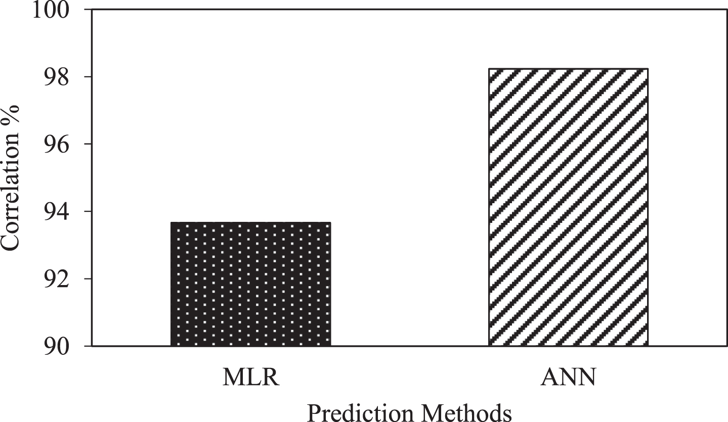
Table 2
Test data for 10 vulnerable sites of Guwahati, Assam, India
| Location | Latitude and longitude | Slope height (m) | Cohesion (kN/m2) | Angle of internal friction (°) | Unit weight of the soil (kN/m3) | Slope inclination (°) | Slope width (m) | FEM | ANN | MLR | |
| Lat. &Long. | H | c | φ | γ | β | m | B | 3D Fcs | Fcs | Fcs | |
| Dhirenpara | 26°09’02.2” N | 15 | 15 | 35 | 18.0 | 60 | 0.200 | 15 | 1.154 | 1.297 | 1.209 |
| 91°43’39.7” E | |||||||||||
| 26°09’04.0” N | 18 | 18 | 35 | 17.9 | 60 | 0.092 | 54 | 1.016 | 1.027 | 1.081 | |
| 91°43’41.2” E | |||||||||||
| Hengerabari | 26°09’06.0” N | 8 | 35 | 25 | 18.0 | 65 | 0.333 | 12 | 1.743 | 1.741 | 1.731 |
| 91°48’15.9” E | |||||||||||
| 26°09’08.9” N | 11 | 48 | 22 | 18.5 | 45 | 0.364 | 16.5 | 2.017 | 2.154 | 2.042 | |
| 91°48’13.3” E | |||||||||||
| Sunsali | 26°11’29.7” N | 10 | 35 | 24 | 18.0 | 70 | 0.067 | 30 | 1.395 | 1.381 | 1.511 |
| 91°47’24.2” E | |||||||||||
| 26°11’32.2” N | 17 | 0 | 37.5 | 18.0 | 45 | 0.059 | 34 | 1.105 | 1.111 | 1.099 | |
| 91°47’27.2” E | |||||||||||
| 26°11’42.8” N | 20 | 46 | 15 | 18.7 | 60 | 0.025 | 80 | 1.047 | 0.997 | 0.881 | |
| 91°47’53.3” E | |||||||||||
| Kharguli | 26°11’37.0” N | 8 | 36 | 0 | 18.0 | 50 | 0.042 | 24 | 1.272 | 1.267 | 1.231 |
| 91°45’40.7” E | |||||||||||
| 26°12’07.2” N | 15 | 47.8 | 0 | 18.0 | 35 | 0.100 | 30 | 1.020 | 1.120 | 1.243 | |
| 91°45’58.4” E | |||||||||||
| 26°11’47.2” N | 20 | 27 | 22 | 17.8 | 40 | 0.100 | 60 | 1.253 | 1.227 | 1.060 | |
| 91°46’06.0” E |
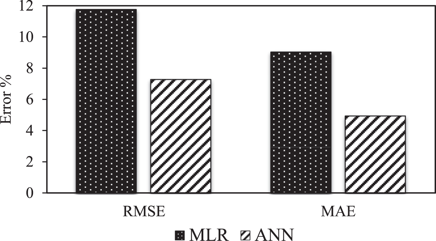
The stability of the prediction models are further checked for error analysis. The error analysis can be performed by computing RMSE and MAE. It can be observed from Fig. 9 that RMSE and MAE values are found to be low particularly for ANN compared to MLR and hence it can be concluded that ANN are able to predict the target values with higher degree of accuracy.
Fig.9
Variation of error percentage for MLR and ANN.
6Conclusion
In this paper, two prediction models have been prepared using multiple regression analysis and artificial neural network to investigate the extent of vulnerability of the hill slopes. This approach is similar to the study performed by Chakraborty and Goswami [8, 9]. But unlike the previous study, the present study involves the development of the prediction models by analyzing 3500 artificial slopes using 3-D finite element method. These prediction models are able to predict the 3-D critical safety factor of slopes. Moreover, in the present study, the pore water pressure is also taken into consideration. Here, six input parameters viz., height of the slope (H), cohesion (c), angle of internal friction (φ), slope inclination (β), unit weight of soil (γ) and dimensionless parameter (m) are used as input parameters whereas the 3-D critical safety factor (Fcs) is used as the output parameter. Levenberg-Marquardt back-propagation algorithm is used for training up the model. To avoid over fitting of the network cross validation technique is used where the whole data set is divided into three distinct subsets viz. training, testing and validation sets. Finally, the validation of the models are done by comparing the results with the analytical results of 10 case studies from in and around the Guwahati city. From the presented results, the following interesting conclusions are drawn:
1. MLR and ANN can act as a good prediction tool for predicting the stability of slopes.
2. The 3-D FOS obtained by the proposed MLR and ANN models are in general agreement with the results from the FEM analyses.
3. The parameters of the prediction model obtained by ANN is found to have a correlation of 98.23% as against 93.66% with MLR.
4. The prediction model obtained by ANN is found to have the lower values of RMSE and MAE of 7.3% and 4.9% respectively, as against 11.7% and 9.0% respectively with MLR. This illustrates that the proposed models are useful alternatives for slope stability analysis.
5. The predicted results of ANN gives higher degree of accuracy compared to MLR.
6. Finally, the results of this study would be very beneficial in the field of decision making for the engineers, planners, developers, etc., by applying the methodology in a GIS in order to estimate stability for a whole study area and create appropriate landslide hazard assessment maps.
References
[1] | Chang M . A 3D slope stability analysis method assuming parallel lines of intersection and differential straining of block contacts. Can Geotech J. (2002) ;39: :799–811. |
[2] | Sakellariou MG , Ferentinou MD . A study of slope stability prediction using neural networks. Geotechnical and Geological Engineering. (2005) ;23: :419–45. |
[3] | Kayesa G . Prediction of slope failure at letlhakane mine with the geomos slope monitoring system. International Symposium on Stability of Rock Slopes in Open Pit Mining and Civil Engineering. (2006) :605–22. |
[4] | Davis TJ , Keller CP . Modelling uncertainty in natural resource analysis using fuzzy sets and Monte Carlo simulation: Slope stability prediction. International Journal of Geographical Information Science. (2010) ;11: (5):409–34. |
[5] | Ahangar-Asr A , Faramarzi A , Javadi AA . A new approach for prediction of the stability of soil and rock slopes. Engineering Computations. (2010) ;27: (7):878–93. |
[6] | Mohamed T , Kasa A , Mukhlisin M . Prediction of slope stability using Statistical Method and Fuzzy Logic. The Online Journal of Science and Technology. (2012) ;2: (4):68–73. |
[7] | Erzin Y , Cetin T . The use of neural networks for the prediction of the critical factor of safety of an artificial slope subjected to earthquake forces. Scientia Iranica. (2012) ;19: (2):188–94. |
[8] | Chakraborty A , Goswami D . Slope stability prediction using Statistical Method. International Journal of Multidisciplinary Research Centre. (2017) a;III: (3):29–35. |
[9] | Chakraborty A , Goswami D . Slope stability prediction using artificial neural network (ANN). International Journal of Engineering and Computer Science. (2017) b;6: (6):21845–8. |
[10] | Michalowski RL . Limit analysis and stability charts for 3D slope failures. Journal of Geotechnical and Geoenvironmental Engineering. (2010) ;136: (4):583–93. |
[11] | Michalowski RL , Martel T . Stability charts for 3D failures of steep slopes subjected to seismic excitation. Journal of Geotechnical and Geoenvironmental Engineering. (2011) ;137: (2):183–9. |
[12] | Gao Y , Zhang F , Lei GH , Li D , Wu Y , Zhang N . Stability charts for 3D failures of Homogenous Slopes. Journal of Geotechnical and Geoenvironmental Engineering, ASCE. (2012) ;139: :1528–38. |
[13] | Lim K , Lyamin AV , Cassidy MJ , Li AJ . Three dimensional slope stability charts for frictional fill materials placed on purely cohesive clay. Int J Geomech ASCE. (2015) ;16: (2). |
[14] | Yilmaz I , Yuksek AG . An example of artificial neural network application for indirect estimation of rock parameters. International Journal of Rock Mechanics and Rock Engineering. (2008) ;41: (5):781–95. |
[15] | Pradhan B . Remote sensing and GIS-based landslide hazard analysis and cross-validation using multivariate logistic regression model on three test areas in Malaysia. Advances in Space Research. (2010) a;45: (10):1244–56. |
[16] | Pradhan B . Landslide Susceptibility mapping of a catchment area using frequency ratio, fuzzy logic and multivariate logistic regression approaches. Journal of the Indian Society of Remote Sensing. (2010) c;38: :301–20. |
[17] | Smith GN . Probability and statistics in civil engineering: An introduction, Collins, London, (1986) . |
[18] | McClelland TL , Rumelhart DE , The PDP Research Group. Parallel Distributed Processing. Cambridge: The MIT Press, (1986) . |
[19] | Demuth H , Beale M . Neural Network Toolbox for Use with MATLAB. The Math Works Inc., Natick, Mass, (1995) . |
[20] | Rumelhart DE , Hinton GE , Williams RJ . Learning internal representations by error propagation. Parallel Data Processing, MIT Press, Cambridge, (1986) , pp. 318–62. |
[21] | Maier HR , Dandy GC . Neural networks for the prediction and forecasting of water resources variables: A review of modeling issues and applications. Environmental Modeling & Software. (2000) ;15: (2000):101–24. |
[22] | Stone M . Cross-validatory choice and assessment of statistical predictions. Journal of Royal Statistical Society. (1974) ;B36: :111–47. |
[23] | Smith M . Neural networks for statistical modeling, Van Nostrand Reinhold, New York, (1993) . |


