
Post-construction settlement estimation and increased earthwork volumes calculation of high loess fill
Abstract
In this study, the post-construction settlement (PCS) area distribution of high fill was analyzed based with reference to a case history of an airport runway crossing a deep gully reclaimed by a thick fill of loess. Earthwork volumes (EV) attributed to PCS was calculated based on in-situ tests. Results showed that the uneven PCS were related to fill depth, construction time, fill rate, integrated compaction degree, and boundary conditions. An empirical equation that considers the aforementioned influence factors was established to calculate the final PCS of high fill. The surface PCS of high fill and the EV can be estimated according to the proposed empirical equation and the original site topography using the three-dimensional finite element method.
1Background
With the recent development of loess engineering in the western region of China, the post-construction settlement (PCS) and the stability of high fill foundations are critical issues because of the transport lines and infrastructures that are constructed on this foundation. Handfelt et al. [17] suggested that in situ testing was the most effective approach to determining the occurrence of the PCS of high fill. Loganathan et al. [25] presented a simple and useful method called field deformation analysis for separating the measured total settlement into immediate compression, primary consolidation, and secondary compression. In addition, this technique considers both settlement and lateral movement. Lee et al. [24] developed a similar method based on laboratory experiments and in situ tests. Clements [5] investigated 68 rockfill dams. When empirical equations were applied, significant errors were generated. Asaoka [3] proposed a useful mathematical method to estimate the PCS of high fill embankment at the early stage. This method was used extensively by [2, 10, 24] in practical engineering. Hyperbolic curves, logarithmic curves, exponential curves, Gompertz curves, and neural network models were used by [34, 25], Yang et al. (2005), and [33] to the PCS in actual engineering applications. The aforementioned methods are regression analysis methods based on time series, and most of these techniques cannot consider other influencing factors.
The influencing factors on the PCS of high fill are complex but are rarely investigated in engineering practice. These factors include the engineering, geological, and hydrological conditions of the original foundation; construction technology; environment; high-fill depth; and the construction time. Many studies focus on numerical analysis; however, most only include a small amount of monitoring data for validation.
A PCS trough of the design elevation plane will occur due to the variable thickness of a high-fill foundation, which must be compensated with increased earthwork volume (IEV). Many researchers have proposed useful methods for earthwork calculation. Easa [6, 7, 9] applied the linear programming method, modified average-end-area method, a mathematical model, and Monte Carlo simulation method to compute earthwork volume. These statements are extensively used in the actual engineering process of balancing cut and fill calculation. Goktepe et al. [15] presented a weighted ground elevation method to minimize the amount of earthwork in the geometric design of highways. Kim et al. (2001) introduced two methods that used vector and parametric representations to either estimate the cross-sectional areas of the excavation precisely or to minimize errors in the calculation of total earthwork cost. With the development of computing and exploration technologies, accurate calculation methods have been established to calculate earthwork volume. Aruga et al. [1] developed a forest road design program based on a high-resolution digital elevation model for a light detection and ranging system. Bao [4] used the digital terrain model of earthwork calculation in land consolidation. Kerry et al. [20] proposed a 3D method of calculating roadway earthwork volume based on 3D laser scanning.
The aforementioned digital methods for computing earthwork volume may be accurate in given geomorphic conditions, but these techniques may be unsuitable for the surface settlement of high fill during consolidation.
Thus, the current study has the potential to estimate the surface PCS of high fill based on large amounts of monitoring data. This work also proposes an empirical equation for computing the final PCS. Then, the IEV may be calculated using 3D finite element method (FEM) using this equation.
2Project review
2.1Project description
Lüliang Airport was located in Shanxi Province. The post-construction deformation of the high fill was investigated in the test section to guide the design and construction of this fill. The fill test was conducted in a deep loess gully that was 700 m long, 50 m to 300 m wide, and 50 m to 100 m deep. The longitudinal slope was 7.1%. The upstream and downstream cross-sections of the valley are denoted by the letters “V” and “U.” The landform and the project profile of the high-fill test section are shown in Fig. 1.
2.2Geological property
The original soil foundation was composed of Q2 loess, Q3 loess, silty clay, and bed rock with sand– shale. The fill material was mainly composed of Q3 and Q2 loess. The physical indices of different soil layers are presented in Table 1. As per the results of the heavy compaction test on the fill, the optimum water content of loess was 13.3%. Its maximum dry density was 1.91 g/cm3.
2.3Design of the high fill
The high fill was divided into three regions, namely, the ordinary, runway pavement, and fill slope regions. Figure 2 shows the design scheme of the high fill. The water content of the fill material was controlled between 11% and 15%, and the compaction degree was maintained between 0.90 and 0.98.
To design the original schemes of foundation treatment, vibration and impact rolling compaction methods were adapted to enhance the compaction degree and the stability of the high fill, as well as those of the original soil foundation. This scenario was provided in Table 2.
The amount of dynamic compaction energy was 3000 kNm. The depth of the treatment varied from 4.0 m to 7.0 m. The ordinary and fill slope regions were compacted using a vibrating roller. First, the runway pavement region was compacted by the vibrating roller. Then, the impact rolling method was applied to increase fill compaction degree when the increased depth of the fill was 1.5 m at each construction circulation. Finally, the dynamic compaction method with an energy level of 3000 kNm was adapted to enhance compaction degree further when the increased depth of the fill was 6.0 m.
3Methods
3.1In situ tests
To determine PCS regularity, the monitoring points of surface settlement are mainly situated on top of the high fill. Digital electronic level was used to monitor the surface settlement. The geometry of the top of the high fill and the location of the monitoring points are displayed in Fig. 3.
The high fill airport was constructed gradually starting from May 2009 and was completed in May 2010. PCS monitoring was initiated at this point. The monitoring process lasted 342 days and was stopped as a result of the implementation of infrastructure construction.
During the construction stage, in situ test data were recorded only once when the increased fill depth was 2 m to 3 m. During the post-construction stage, these data were registered once every 10 days during the first 3 months, once every 15 days during the middle 6 months, and once every 30 days during the final 3 months.
3.2IEV calculation with FEM
In high fill engineering, the parameter related to fill elevation and compaction degree must be designed. However, the average fill rate, construction time, and weather conditions are stable when duration time was considered. The PCS of high fill varies in a wide range. Thus, volume loss as a result of PCS must be compensated with increased earthwork up to the designed elevation.
In theory, the contour curves of the topography of the original loess gully, design elevation of high fill, and PCS should first be obtained to calculate IEV accurately. The 3D coordinates of this scenario can be expressed as follows: Z(Xi,Yi,HD), Z(Xi,Yi,Hi), and Z(Xi,Yi,Hsi). These coordinates are displayed in Fig. 4.
HD was the design elevation of the top of the high fill; Hi was the elevation of the original loess gully; and Hs was the elevation of the top of the high fill as a result of PSC. The depth of high fill H was equal to HD – Hi. The PCS SDi was equal to HD – Hsi.
Figure 4 illustrates the settlement trough of the high fill and the landform of the original loess gully. The surface of the design elevation of the high fill (ZD), surface of the landform of the original loess gully (Z0), and surface generated through PCS (Zs) are expressed in 3D coordinate systems using the following equations:
(1)
(2)
(3)
The volume of high fill can be expressed as follows:
(4)
The IEV attributed to PCS can be written as follows:
(5)
These equations cannot be expressed by an explicit equation given the irregular surface of the loess gully and the top of the high fill. However, the IEV can be calculated using FEM with ANSYS software. The detailed computing processes are presented in the subsequent section.
4Results and discussion
4.1Influence of duration time on PCS
The hyperbolic curve was used to estimate and determine the relationship between PCS and duration time based on finite monitoring data. The compression ratio S/H was defined to compute the total vertical strain of the high fill and foundation. S was the PCS of the top of the high fill, and H was fill depth. Figure 5 shows the curves of S/H (mm/m) versus duration time D (days) as per the monitoring data of the key points positioned on the top of the high fill.
The average curve of S/H versus duration time D can be expressed as follows:
(6)
The figures indicate that the compression ratio of the high fill surface increased over time and remained stable after three years. In the P-2, for example, the stable PCS value was 487.0 mm and the uncompleted PCS value was 164.0 m (the completed PCS was 323.0 mm over 342 days).
4.2Influence of fill depth and rate on PCS
We suppose that t (days) was the average fill duration time. v (m/day) was the average fill rate, which was equal to H/t. v varies from 0.05 m/day to 0.42 m/day, as illustrated in Fig. 6. The relationship between the surface PCS and either fill depth or fill rate was determined using the statistical analysis method on the basis of PCS monitoring data and fill records, as indicated in Fig. 7(a) and (b).
Figure 7(a) shows that the curve of PCS versus fill depth can be fitted with Equation (7) as follows:
(7)
Figure 7(b) suggests that the relationship between the PCS of the high fill and average fill rate can be expressed as follows:
(8)
This equation indicates that the PCS of the high fill increased linearly with an increase in the average fill depth. Moreover, the PCS of the high fill increased exponentially with an increase in the average fill rate. Therefore, fill rate should be reasonably controlled to reduce PCS and to meet the requirements of high fill.
4.3Influence of compaction degree on PCS
Compaction degree influences the PCS of the high fill. The actual compaction degrees of the high fill in different regions and elevations were detected and contrasted with that of the design. Figure 8 suggests that the local minimum compaction degree was 5% lower than that of the design, that the maximum value was 2% higher than that of the design, and that the actual compaction degree was 1% lower than the standard design requirements.
We suppose that integrated compaction degree (k) reflected the degree of fill and foundation treatment. This variable can be expressed as follows:
(9)
Thus, the relationship between compression ratio and fill depth can be determined using the statistical analysis method, as illustrated in Fig. 9. Compression ratio decreased with an increase in fill depth at the same compaction degree area. Nonetheless, further analysis suggests that compression ratio also decreased with an increase in integrated compaction degree, as displayed in Fig. 10. The relationship between compression ratio and integrated compaction degree can be expressed as in Equation (10):
(10)
In addition, the integrated compaction degree increased by 3% and the compression ratio decreased by 10% to 50%. Thus, the PCS of the high fill can be effectively reduced by increasing the integrated compaction degree during the construction stage.
4.4Empirical equation of PCS
The previously presented results show that the PCS of the high fill was closely related to fill duration time under step loading (t), fill depth (H), average fill rate (υ), integrated compaction degree (k), post-construction time (D), and geomorphic conditions. Thus, PCS can be expressed as follows:
(11)
The proposed empirical equations reflected the actual interaction effects among the aforementioned influence factors. When large volumes of statistical monitoring data regarding the PCS, step filling process, and integrated compaction degree during construction are summarized (Table 3), the PCS of the high fill that was associated with υ, k, H, and D can be expressed as in Equation (12):
(12)
The maximum error between the monitored PCS and the estimated PCS was 17%. The average error was 8%. Therefore, the estimation error determined using the empirical equation [Equation (12)] can satisfy the requirements of major geotechnical engineering design.
4.5Estimation and validation of IEV
On the basis of the FEM, the calculation process of the IEV can be expressed in the following steps:
(1) The parameters υ, k, and H are obtained according to the daily fill records. Furthermore, PCS (SD) can be calculated using Equation (12) when duration time D = 100 years. Key points are selected to estimate the PCS for calculating IEV. The analysis results are listed in Table 4, and the XOY coordinate system was exhibited in Fig. 3.
(2) As per Table 3, the 3D coordinate system of the key points (X, Y, SD) can be imported into FE software. The irregular surface attributed to PCS can be fitted with a triangulated irregular network on the basis of the key points. The volume between the design elevation plane and the fitted irregular surface was determined. Then, the FEM of the IEV was meshed with the element type named SOLID45. All of the meshed element volumes are calculated using ANSYS Parametric Design Language.
(3) The calculated IEV was the designed volume of the compacted soil that fills the settlement trough. The actual IEV was the cut volume of the original soil. As such, the design compaction degree and the natural density of the original soil are considered in the computation of the actual IEV.
The test section of the Lüliang Airport was taken as an example. The FEM of the IEV attributed to PCS can be meshed as depicted in Fig. 11.
Given the 3D finite element mesh, IEV can be exported from ANSYS software. IEV Vs was calculated to be 6398 m3. When the coefficient of volumetric expansion and the compaction degree of the fill are considered, the actual IEV V was calculated as follows:
(13)
Where, V was the actual IEV. ρdmax was the maximal dry density of the loess, which was equal to 1910 kg/m3. wop was the optimum water content of the loess, which was equal to 13.3%. ρ0 was the natural density of the undisturbed loess, which was equal to 1710 kg/m3. k was the design compaction degree of the loess, which was equal to 98% of the optimum density. As such, the actual IEV was calculated as 6398 m3 × 1910 × (1 + 13.3%) × 98% /1710 = 7935 m3 .
As per the calculated IEV, the settlement trough of the top of the test section was filled with natural Q3 loess 1.2 years after the completion of the project. This trough was generated by PCS. The final actual IEV was 8122 m3 and was greater than the estimated volume because of the volume lost during transport, error in natural density, controlled compaction degree, and calculation method. In summary, the calculated volume was similar to the actual volume, thus indicating that the arithmetic mean was effectively applied to earthwork engineering.
5Conclusions
The estimation of PCS was investigated based on in situ tests and FEM. Moreover, the IEV of the high fill was calculated. The following conclusions can be drawn:
(1) The PCS of the high fill was not only relevant to post-construction time but also to construction time, average fill rate, fill depth, average compaction degree, and the original topographic conditions. Hyperbolic and linear curves can be used to estimate compression ratio versus duration time and versus integrated compaction degree, respectively. The relationship between the PCS and fill depth can be analyzed using linear regression. The curve of PCS versus average fill rate can be expressed as an exponential equation.
(2) The empirical equation of PCS was established through the statistical analysis of numerous monitoring data. These data include fill depth, average compaction degree, average fill rate, and construction time. The proposed empirical equation can meet the requirements of the engineering design. Moreover, the FEM method based on this equation was simply used to calculate IEV when the shape of the surface was irregular as a result of PCS. The amount of IEV estimations were close to the indeed values in this work, it shows that the estimation method using FEM is suitable for the high fill loess in the gully.
(3) The empirical equation of PCS proposed in this work may be suitable for the engineering applications with specific design and construction technologies and under particular geographic conditions. The coefficient of the empirical equation may be modified in other projects. Moreover, the IEV calculation method based on FEM may be inaccurate as a result of either the PCS estimation error or the volume loss of earthwork during transport. This issue will be the topic of subsequent research.
Conflict of interest
The author(s) declare(s) that there is no conflict of interest regarding the publication of this paper.
Acknowledgments
Financial supports from the National Natural Science Foundation of China (Grant No. 51308456), and from the Project of Scientific Research of Shaanxi (Grant No. 2013JQ7022 and 2015JM5175) and from the Postdoctoral fund of shaanxi province are gratefully acknowledged. The authors wish to thank the research team of Geotechnical Institute of Xi’an University of Technology for their assistance during the in-situ tests. The authors acknowledge thoughtful and helpful comments from the reviewers.
References
[1] | Arulrajah A , Bo MW . Factors affecting consolidation related prediction of singapore marine clay by observational methods. Geotechnical and Geological Engineering. (2008) ;26: (4):417–30. |
[2] | Sallam AM , Jammal SE . Case history: Finite element analysis of time dependent settlement of Lake Jessup Bridge Embankment in Central Florida. GeoFlorida. (2010) )2182–91. |
[3] | Aruga K , Sessions J , Akay AE . Application of an airborne laser scanner to forest road design with accurate earthwork volumes. Journal of Forest Research. (2005) ;10: (2):113–23. |
[4] | Asaoka A . Observational procedure of settlement prediction. Soils and Foundations. Japanese Geotechnical SOC. (1978) ;18: (4):87–101. |
[5] | Bao Y . Applications of the MapGIS-based Digital Topographic Model on Earthwork Calculation on Land Consolidation. Proceeding of International Conference on Computer Distributed Control and Intelligent Environmental Monitoring, (2011) , China. |
[6] | Clements RP . Post-construction deformation of rockfill dams. Journal of Geotechnical Engineering. ASCE. (1984) ;110: (7):821–40. |
[7] | Easa S . Selection of roadway grades that minimize earthwork cost using linear programming. Transportation Research. (1988) ;22: (2):121–36. |
[8] | Easa S . Discussion of cut and fill calculations by modified average-end-area method by James W. Epps and Marion W.Corey. Journal of Transportation Engineering. (1992) ;118: (4):600–1. |
[9] | Easa S . Estimating earthwork volumes of curved roadways-mathematical model. Journal of Transportation Engineering. (1992) ;118: (6):834–49. |
[10] | Easa S . Estimating earthwork volumes of curved roadways-simulation model. Journal of Surveying Engineering. (2003) ;129: (1):19–27. |
[11] | Matyas EL , Rothenburg L . Estimation of total settlement of embankments by field measurements. Canadian Geotechnical Journal. (1996) ;33: (5):834–41. |
[12] | Eyubov AA . Creep of collapsible loess soil under overall compression. Soil Mechanics and Foundation Engineering. (1986) ;23: (3):121–5. |
[13] | Garlanger JE . The consolidation of soils exhibiting creep under constant effective stress. Geotechnique. (1972) ;22: (1):71–8. |
[14] | Goktepe AB , Lav AH . Method for balancing cut-fill and minimizing the amount of earthwork in the geometric design of highway. Journal of Transportation Engineering. (2003) ;129: (5):564–71. |
[15] | Graham J , Crooks JHA , Bell AL . Time effects on the stress-strain behaviour of natural soft clays. Geotechnique. (1983) ;33: (3):327–40. |
[16] | Zhu G , Yin J-H , Graham J . Consolidation modeling of Soil under the test embankment at Chek Lap Kok international airport in Hong Kong using a simple finite method. Can Geoteeh. (2001) ;38: , 349–63. |
[17] | Handfelt LD , Koutsoftas DC , Foott R . Instrumentation for high fill in Hong Kong. Journal of Geotechnical Engineering, ASCE. (1987) ;113: (GT2):127–46. |
[18] | Huang W , Fityus S , Bishop D , Smith D , Sheng D . Finite-element parametric study of the consolidation behavior of a trial embankment on soft clay. Int J Geomech. (2006) ;6: (5):328–41. |
[19] | Zornberg JG , McCartney JS . Centrifuge permeameter for unsaturated soils. I: Theoretical basis and experimental developments. J Geotech Geoenviron Eng. (2010) ;136: , 1051–63. |
[20] | Karim MR , Gnanendran CT , Lo SCR , et al. Predicting the long-term performance of a wide embankment on soft soil using an elastic-viscoplastic model. Canadian Geotechnical Journal. (2010) ;47: (2):244–57. |
[21] | Kerry TS , Dianne KS , James PP . Road construction earthwork volume calculation using three-dimensional laser scanning. Journal of Surveying Engineering. (2012) ;138: (2):96–9. |
[22] | Kim E , Schonfeld P . Estimating Highway Earthwork Cross Sections Using Vector and Parametric Representation. Proceeding of TRB 2001 Annual Meeting, Washington DC, (2001) . |
[23] | Kim Y , Leroueil S . Modeling the viscoplastic behaviour of clays during consolidation: Application to Berthierville clay in both laboratory and field conditions. Canadian Geotechnical Journal. (2001) ;38: (3):484–97. |
[24] | Lee D , Jeong S . A consolidation settlement prediction considering primary and secondary consolidation. Journal of The Korean Society of Agricultural Engineers. (2005) ;47: (1):61–8. |
[25] | Liu H , Li P-F , Zhang Z-Y . Prediction of the post-construction settlement of the high embankment of Jiuzhai— Huanglong airport. Chinese Journal of Geotechnical Engineering. (2005) ;27: (1):61–8. |
[26] | Lo KY , Bozozuk M , Law KT . Settlement analysis of the Gloucester high fill. Canadian Geotechnical Journal. (1976) ;13: (4):339–54. |
[27] | Loganathan N , Balasubramaniam A , Bergado D . Deformation analysis of embankments. J Geotech Engrg. (1993) ;119: (8):1185–206. |
[28] | Lollino P , Cotecchia F , Zdravkovic L , Potts D . Numerical analysis and monitoring of Pappadai dam. Canadian Geotechnical Journal. (2005) ;42: (6):1631–43. |
[29] | Mesri G , Choi Y . Settlement analysis of embankments on soft clays. J Geotech Engrg. (1985) ;111: (4):441–64. |
[30] | Nagahara H , Fujiyama T , Ishiguro T , et al. FEM analysis of high airport embankment with horizontal drains. Geotextiles and Geomembranes. (2004) ;22: (1):49–62. |
[31] | Venda Oliveira PJ , Lemos LJL , Coelho PALF . Behavior of an atypical embankment on soft soil:Field observations and numerical simulation. Journal of Geotechnical and Geo-environmental Engineering, ASCE. (2010) ;136: (1):35–47. |
[32] | Robert YK , Liang , Mitchell JK . Centrifuge evaluation of numerical model for clay. Journal of Geotechnical Engineering. (1988) ;114: (3):265–83. |
[33] | Borja RI . Generalized creep and stress relaxation model for clays. Journal of Geotechnical Engineering. (1992) ;118: (11):1765–86. |
[34] | Tan SA . Hyperbolic method for settlements in clays with vertical drains. Can Geotech J. (1994) ;31: , 125–31. |
[35] | Shahin MA , Maier HR , Jaksa MB . Predicting settlement of shallow foundations using neural networks. Journal of Geotechnical and Geo-environmental Engineering. (2003) ;129: (12):1175–77. |
Figures and Tables
Fig.1
Profile of the high-fill test section in Lüliang Airport.
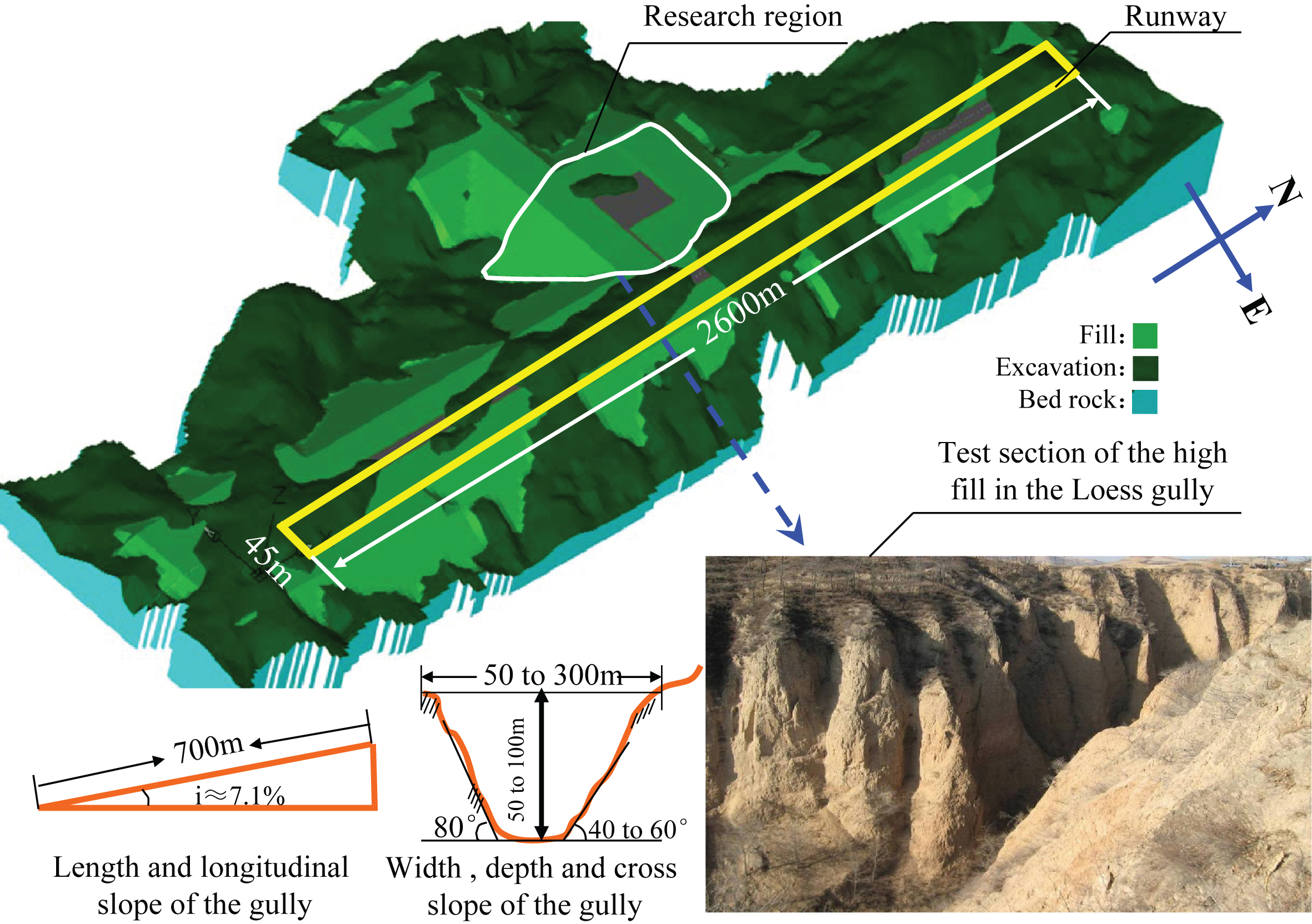
Fig.2
Design of the high fill with different compaction degree (k).
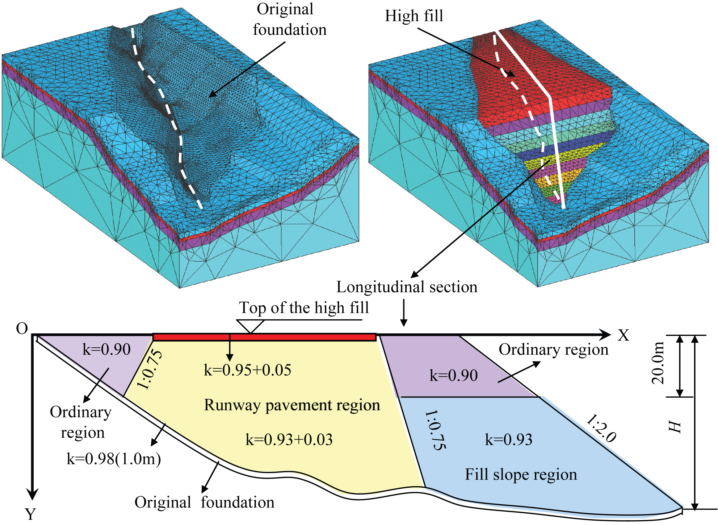
Fig.3
Surface monitoring points of the high fill.
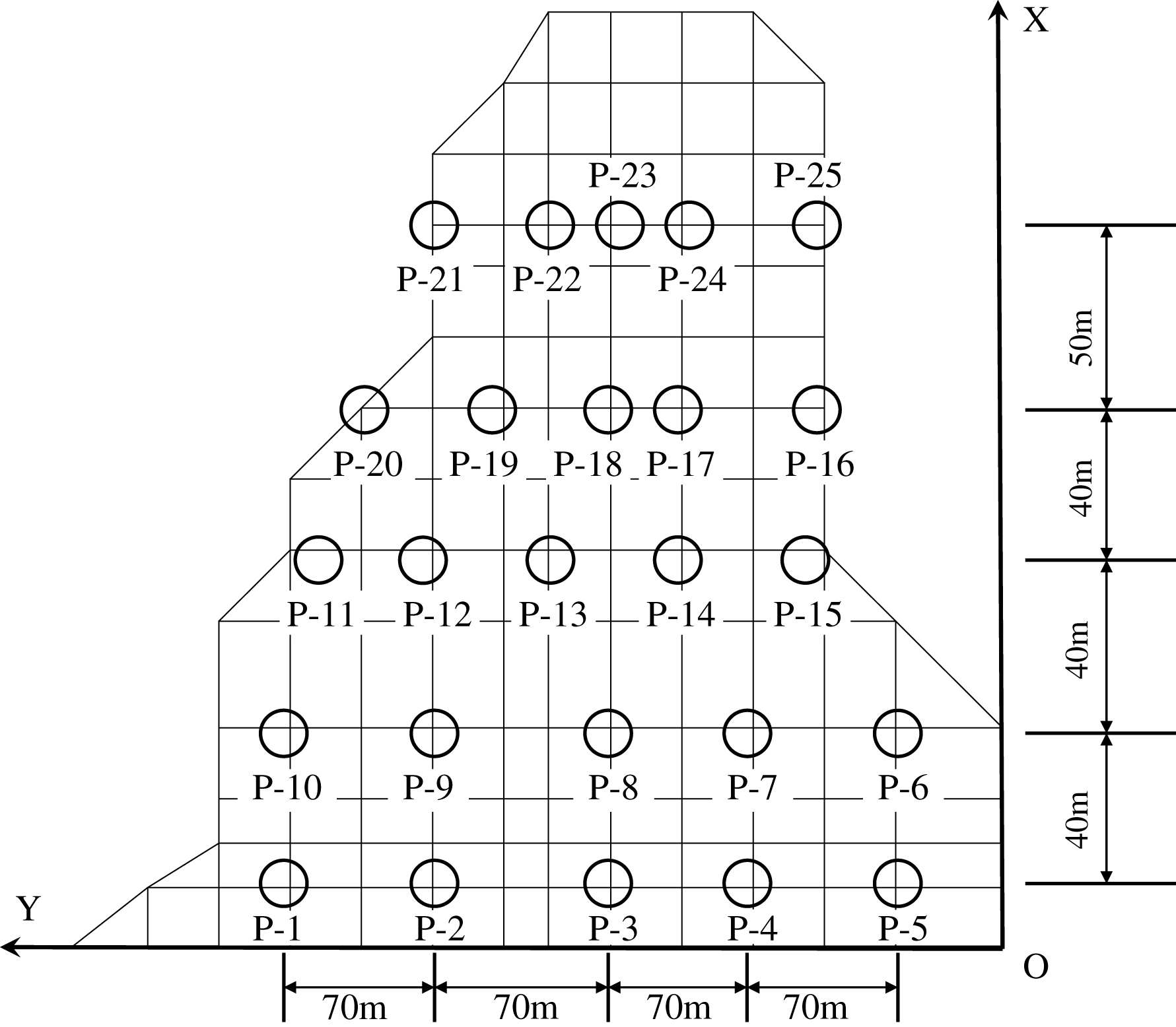
Fig.4
Calculation of the resultant IEV from PCS.
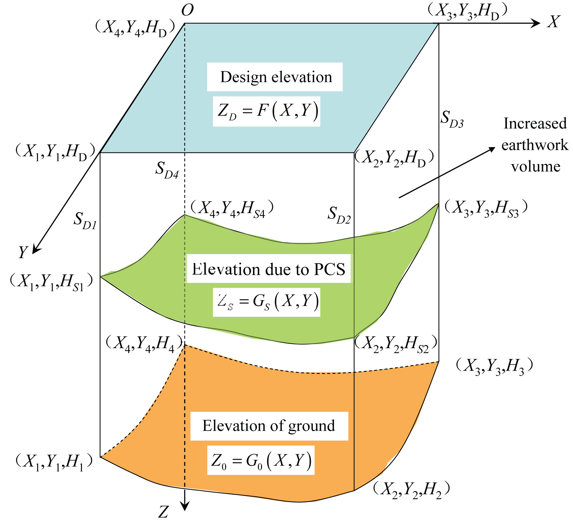
Fig.5
Curves of S/H versus duration time D of the key points.
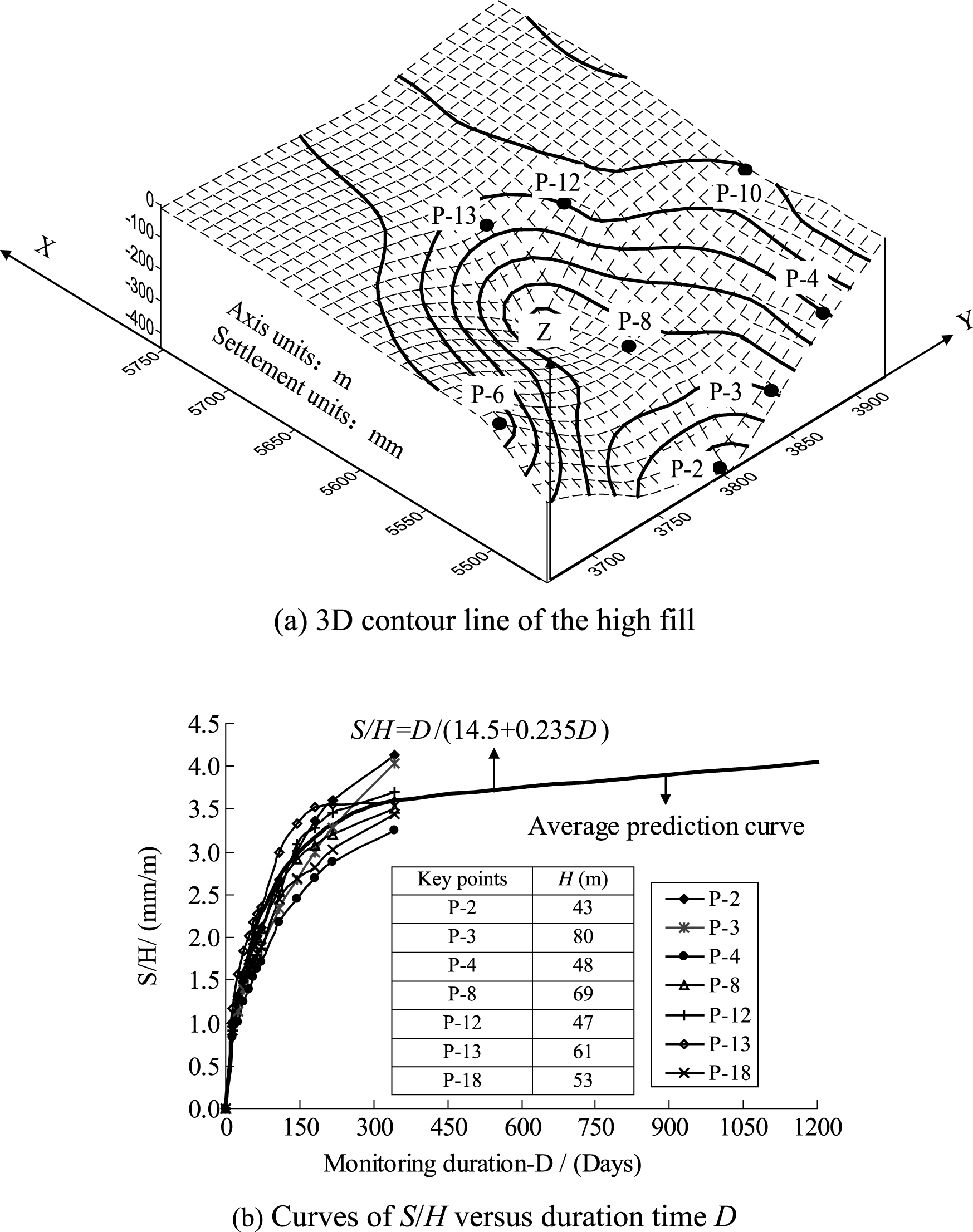
Fig.6
Average fill rate of the high fill.
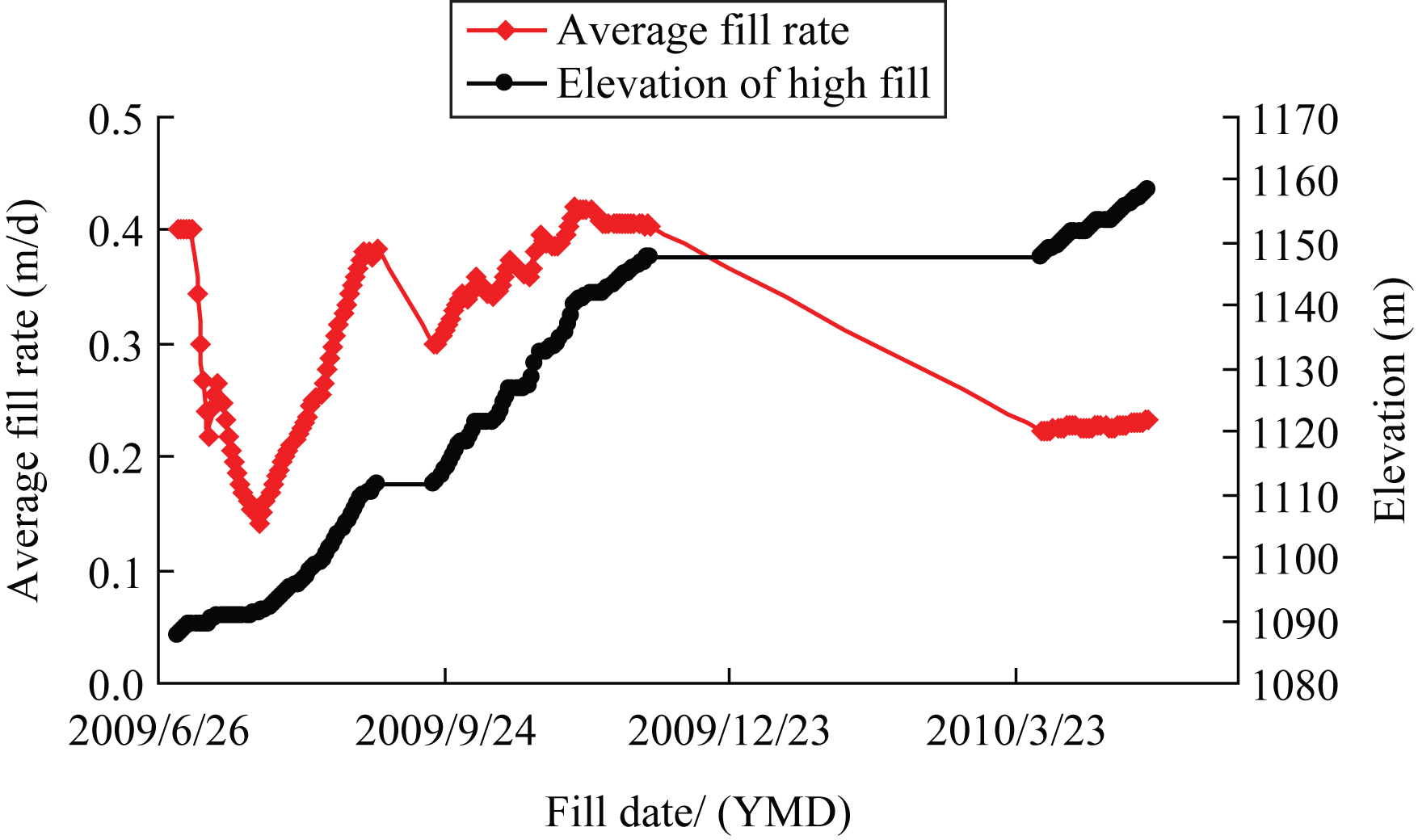
Fig.7
PCS versus fill depth and fill rate.
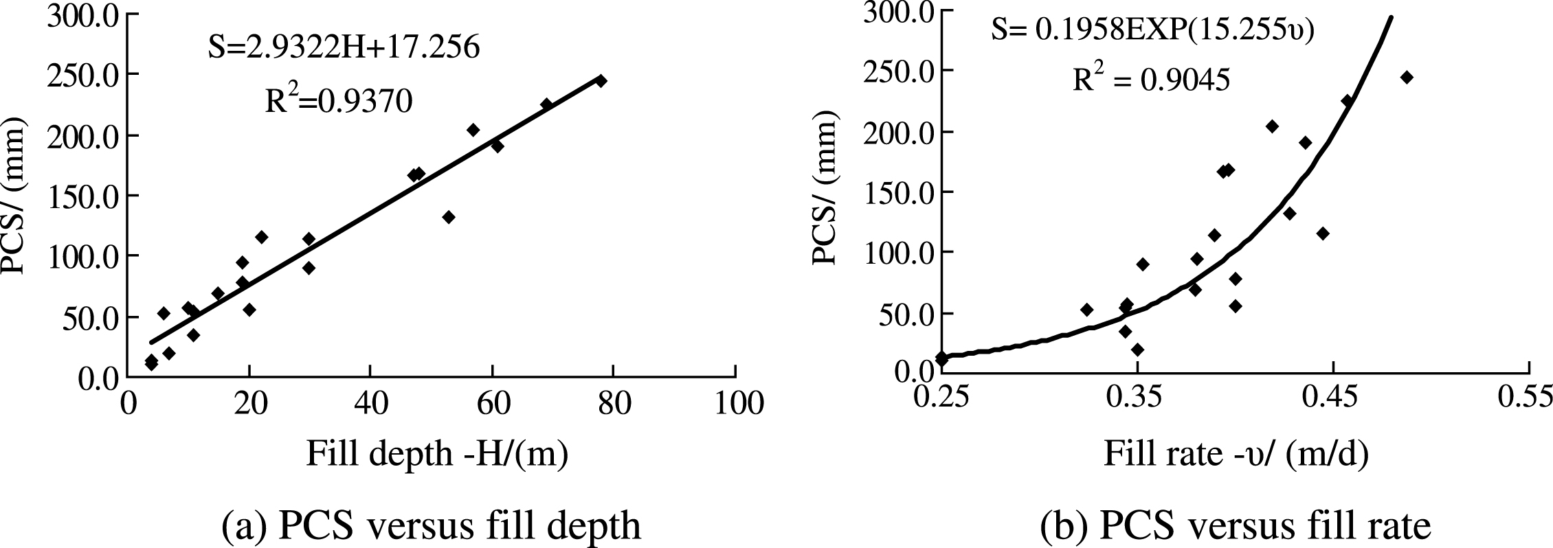
Fig.8
Design compaction degree versus measured data.
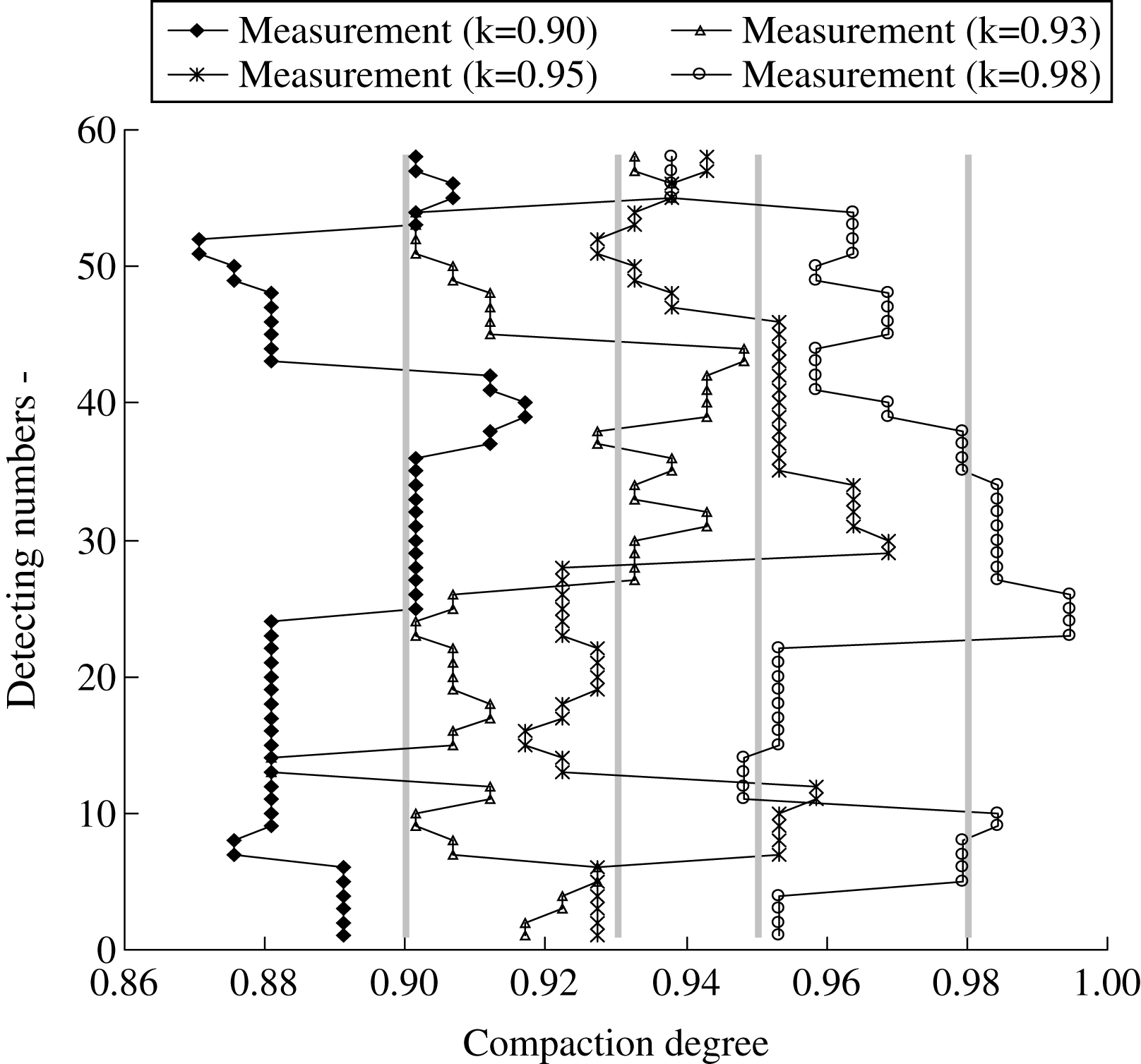
Fig.9
S/H versus H.
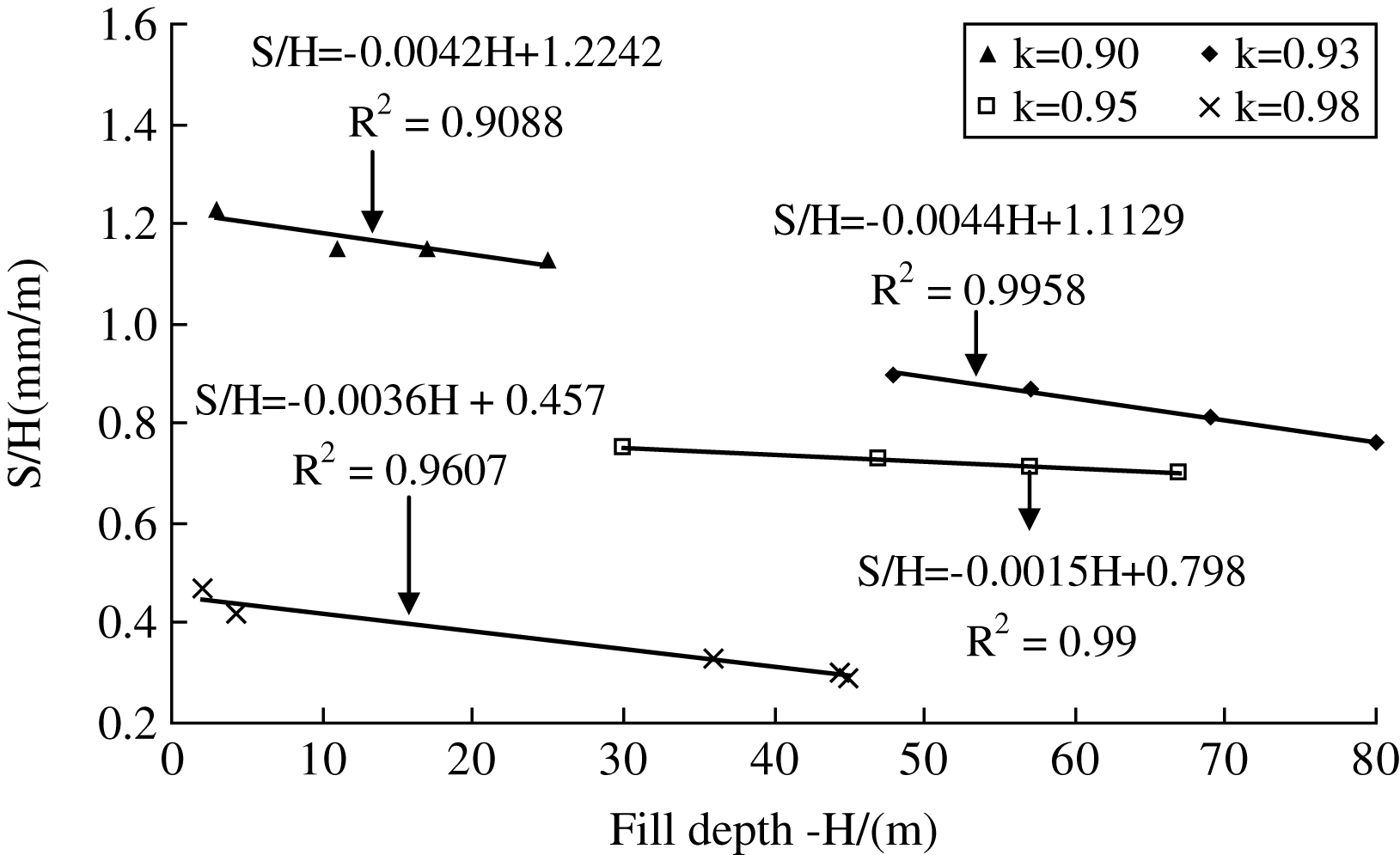
Fig.10
S/H versus k.
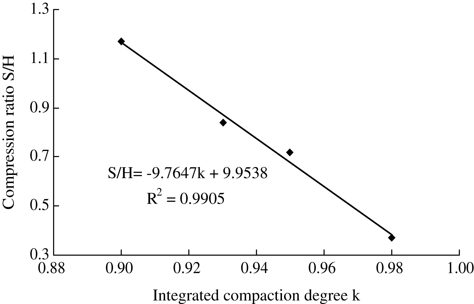
Fig.11
Calculation of the IEV by FEM.
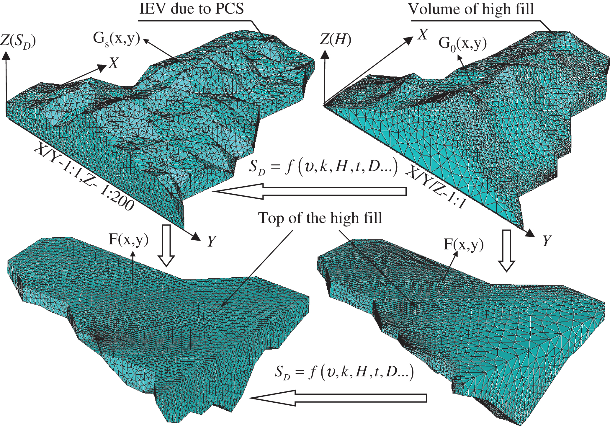
Table 1
Parameters of different layer soil
| Layer | Water content w(%) | Dry density ρd(g/cm3) | Void ratio e | Liquid limit wl(%) | Plastic limit wp(%) | Thickness (m) |
| ①1 Q42ml | 23.66 | 1.60 | 0.696 | 25.2 | 15.89 | 1.7∼6.5 |
| ①2 Q4dl | 15.65 | 1.44 | 0.882 | 24.72 | 15.75 | 1.5∼19.3 |
| ②1 Q3eol | 15.84 | 1.63 | 0.663 | 24.98 | 16.21 | 6.5∼17.8 |
| ②2 Q3eol | 16.97 | 1.56 | 0.741 | 24.87 | 16.08 | 3.1∼21.5 |
| ③Q2eol | 21.36 | 1.65 | 0.647 | 29.29 | 17.49 | 2.9∼14.6 |
| ④1 N2b | 22.00 | 1.64 | 0.663 | 29.91 | 17.53 | 12.0∼19.5 |
| ④2 N2b | 21.53 | 1.67 | 0.628 | 30.13 | 17.66 | 13.5∼24.6 |
Table 2
Fill methods and compaction degree control standards of high fill
| Regions | Below runaway pavement | Compaction method | Loose laying depth | Compaction degree | Fill material |
| Runaway pavement | 0∼1 m | vibration and impact rolling | 4 × 0.35 m,1.0 m | 0.93+0.05 | Q2 loess |
| 1∼20 m | vibration and impact rolling | 5 × 0.4 m,1.5 m | 0.93+0.03 | Q3 loess | |
| 20 m∼H | vibration rolling and dynamic compaction | 20 × 0.4 m,6.0 m | |||
| Fill slope | 0∼20 m | vibration rolling | 0.4 m | 0.90 | Q2,Q3 loess |
| 20 m-H | 0.4 m | 0.93 | |||
| Ordinary | 0∼1 m | 3 × 0.45 m | 0.90 | Q3 loess | |
| 1 m∼H | 0.5 m | Q2,Q3 loess |
Table 3
Estimation of the PSC of the monitoring points using Equation (12)
| Key points | H (m) | t (days) | v (m/d) | k | D = 217 days Monitoring -S (mm) | D = 217 days Estimation-S (mm) | Absolute error |
| P-3 | 78 | 219 | 0.36 | 90% | 244.1 | 264.0 | 8% |
| P-4 | 48 | 155 | 0.31 | 91% | 167.7 | 155.7 | 7% |
| P-5 | 4 | 16 | 0.25 | 90% | 19.0 | 17.9 | 6% |
| P-6 | 7 | 20 | 0.35 | 91% | 50.1 | 47.8 | 5% |
| P-8 | 69 | 291 | 0.24 | 94% | 204.4 | 193.9 | 5% |
| P-9 | 57 | 136 | 0.42 | 93% | 224.7 | 238.1 | 6% |
| P-10 | 10 | 25 | 0.40 | 95% | 87.3 | 85.2 | 2% |
| P-11 | 15 | 40 | 0.38 | 96% | 78.5 | 82.1 | 5% |
| P-12 | 47 | 120 | 0.39 | 95% | 166.7 | 178.5 | 7% |
| P-13 | 61 | 211 | 0.29 | 93% | 190.1 | 182.0 | 4% |
| P-14 | 30 | 77 | 0.39 | 93% | 114.5 | 134.1 | 17% |
| P-15 | 19 | 48 | 0.40 | 92% | 104.8 | 113.0 | 8% |
| P-16 | 11 | 32 | 0.34 | 90% | 51.3 | 57.8 | 13% |
| P-17 | 20 | 65 | 0.31 | 91% | 65.2 | 73.0 | 12% |
| P-18 | 53 | 210 | 0.25 | 92% | 142.3 | 158.3 | 11% |
| P-19 | 30 | 100 | 0.30 | 90% | 90.4 | 102.8 | 14% |
| P-22 | 19 | 48 | 0.40 | 88% | 112.4 | 118.0 | 5% |
| P-23 | 22 | 55 | 0.40 | 90% | 115.2 | 124.5 | 8% |
| P-24 | 11 | 32 | 0.34 | 89% | 54.3 | 58.5 | 8% |
| P-25 | 4 | 16 | 0.25 | 90% | 16.4 | 17.9 | 9% |
Table 4
Estimation of PCS for earthwork volume calculation
| No. | X (m) | Y (m) | k | υ (m/day) | H (m) | SD (mm) | No. | X (m) | Y (m) | k | υ (m/day) | H (m) | SD (mm) |
| 1 | 61.5 | 0.0 | 96% | 0.29 | 10.61 | –44.9 | 70 | 111.5 | 127.5 | 0.900 | 0.41 | 69.43 | –318.6 |
| 2 | 111.5 | 50.0 | 96% | 0.29 | 10.94 | –46.0 | 71 | 91.5 | 127.5 | 0.930 | 0.41 | 59.04 | –269.6 |
| 3 | 263.0 | 70.0 | 96% | 0.29 | 12.01 | –49.4 | 72 | 61.5 | 127.5 | 0.930 | 0.41 | 59.86 | –272.4 |
| 4 | 243.0 | 50.0 | 91% | 0.29 | 10.00 | –46.4 | 73 | 41.5 | 127.5 | 0.930 | 0.42 | 70.57 | –320.1 |
| 5 | 243.0 | 140.0 | 92% | 0.29 | 13.61 | –58.3 | 74 | 29.0 | 127.5 | 0.930 | 0.43 | 74.19 | –345.5 |
| 6 | 263.0 | 127.5 | 90% | 0.29 | 12.53 | –56.1 | 75 | 16.5 | 127.5 | 0.930 | 0.44 | 74.05 | –360.2 |
| 7 | 223.0 | 160.0 | 90% | 0.29 | 17.18 | –72.9 | 76 | 0.0 | 127.5 | 0.930 | 0.42 | 74.66 | –334.1 |
| … | … | … | … | … | … | … | … | … | … | … | … | … | … |
| 54 | 111.5 | 140.0 | 90% | 0.33 | 59.61 | –235.4 | 123 | 131.5 | 50.0 | 0.930 | 0.41 | 14.45 | –117.2 |
| 55 | 131.5 | 140.0 | 90% | 0.29 | 46.21 | –177.8 | 124 | 61.5 | 50.0 | 0.930 | 0.41 | 38.84 | –200.5 |
| 56 | 151.5 | 140.0 | 90% | 0.29 | 33.13 | –130.6 | 125 | 41.5 | 50.0 | 0.930 | 0.41 | 38.84 | –200.5 |
| 57 | 171.5 | 140.0 | 90% | 0.29 | 29.03 | –115.8 | 126 | 29.0 | 50.0 | 0.930 | 0.41 | 29.72 | –169.3 |
| 58 | 191.5 | 160.0 | 90% | 0.29 | 17.09 | –72.4 | 127 | 16.5 | 50.0 | 0.900 | 0.41 | 29.72 | –175.2 |
| 59 | 191.5 | 140.0 | 96% | 0.29 | 27.39 | –99.0 | 128 | 0.0 | 50.0 | 0.900 | 0.41 | 25.20 | –158.8 |
| 60 | 203.0 | 160.0 | 96% | 0.29 | 16.11 | –62.7 | 129 | 0.0 | 30.0 | 0.910 | 0.41 | 14.58 | –119.5 |
| 61 | 203.0 | 140.0 | 96% | 0.29 | 21.91 | –81.3 | 130 | 0.0 | 0.0 | 0.900 | 0.41 | 2.32 | –76.2 |
| 62 | 223.0 | 140.0 | 96% | 0.29 | 15.32 | –60.1 | 131 | 16.5 | 30.0 | 0.900 | 0.41 | 15.72 | –124.6 |
| 63 | 243.0 | 127.5 | 96% | 0.29 | 13.74 | –55.0 | 132 | 16.5 | 0.0 | 0.900 | 0.41 | 6.32 | –90.6 |
| 64 | 223.0 | 127.5 | 96% | 0.29 | 18.85 | –71.5 | 133 | 29.0 | 30.0 | 0.920 | 0.41 | 21.61 | –143.0 |
| 65 | 203.0 | 127.5 | 95% | 0.41 | 28.92 | –162.8 | 134 | 29.0 | 0.0 | 0.940 | 0.41 | 8.34 | –95.7 |
| 66 | 191.5 | 127.5 | 94% | 0.41 | 32.60 | –177.1 | 135 | 41.5 | 30.0 | 0.926 | 0.41 | 24.49 | –152.1 |
| 67 | 171.5 | 127.5 | 95% | 0.41 | 39.37 | –197.2 | 136 | 41.5 | 0.0 | 0.930 | 0.41 | 8.68 | –97.4 |
| 68 | 151.5 | 127.5 | 92% | 0.41 | 50.34 | –243.7 | 137 | 61.5 | 30.0 | 0.961 | 0.29 | 20.48 | –76.7 |
| 69 | 131.5 | 127.5 | 90% | 0.41 | 61.17 | –288.8 | 70 | 111.5 | 127.5 | 0.900 | 0.41 | 69.43 | –318.6 |


