
Shear strength of granular soils from the simulation of dynamic penetration tests
Abstract
This paper presents a model for the numerical simulation of dynamic penetration tests in cohesionless soils. In the model, dynamic penetration equations are solved by finite difference analysis in the time domain to produce the discretization of the penetration system. The approach allows essential effects of the soil influence to be accounted for, including the dynamic soil resistance by viscous damping during penetration. The model performance has proved by comparisons between the static and dynamic resistance to reproduce the variation with time of measured force, velocity, displacement and energy associated with the interaction mechanism around split-spoon samplers when penetrating in the ground. A realistic representation of the dynamic penetration mechanism allows the internal friction angle of the soil to be estimated. The proposed methodology accounts for scale effects and produces values of φ′ within the same order of magnitude as those estimated from piezocone test data.
1Introduction
Dynamic penetration testing, which plays an important role in the field of site investigation, is performed in engineering practice to provide assessment of the in situ properties of soils. Dynamic tests such as the SPT (Standard Penetration Test), LPT (Large Penetration Tests) and BPT (Becker Penetration Tests) are driven into the soil by means of an impact force applied to a rod stem, while recording the overall displacement at the rod head. Given the fact that displacement is the only measurement in these tests, interpretation methods of recorded results are empirical and supported by simple guidelines. This practice is in contrast with the developments in the interpretation of pile drivability where the analysis is made on the basis of wave propagation theory (e.g. Smith [1]; Poulos and Davis [2]; Deeks [3]; Randolph and Bruno [4]).
Although it has been generally recognized that the practice and analysis of dynamic penetration tests has to be improved, there have been relatively few research efforts devoted to rational methods of interpretation. Most related research was carried out in the 1970’s and early 80’s. A major focus of the research was the variability in energy delivered to the rods by the hammer. Schmertmann and Palacios [5] showed experimentally that penetration resistance varies inversely with the energy transmitted to the rods by a hammer impact up to an N-value of 50. Seed et al. [6] and Skempton [7] suggested that the measured blow counts (or N-value) should be corrected to a standard energy. Based on the estimate that most empirical relationships in use at that time had been developed with systems delivering about 60% of the maximum potential energy of the SPT hammer, a reference value of 60% was assumed. As research has shown that different hammers deliver differing levels of energy, the measurement of stress wave energy during driving, at a location just below the anvil, is now a common means of quality control for SPT results.
Odebrecht et al. [8] and Schnaid et al. [8, 10] reconsidered the energy transfer in the SPT and suggested that the effective energy is greater than the stress wave energy. They expressed the effective sampler energy as a function of the hammer height of fall, sampler permanent penetration and weight of both hammer and rod stem. The energy delivered to the rod stem was used by Odebrecht et al. [8] to calculate the dynamic reaction force (Fd) applied to the soil during sampler penetration using the principles of energy conservation. This opened up the possibility of using the dynamic reaction force to derive the shear strength properties of cohesionless soils.
The present paper extends these concepts by introducing a numerical 1-D routine developed to model the interaction of the sampler with the soil during dynamic penetration testing in cohesionless soils using different sampler and hammer configurations. Focus is placed on capturing the interaction mechanism around split-spoon samplers as they penetrate in the ground. The analysis uses the concepts of energy conservation, dynamic equilibrium and cavity expansion theory. Dimensional analysis concepts are applied to develop a sampler-soil interaction model named Dimensionless Smith’s Model. The model results are discussed with the aim of (a) producing a better understanding of the sampler soil-interaction mechanism and (b) estimating soil parameters in cohesionless geomaterials.
2Dynamic penetration model
Theoretical solutions for the motion produced in an elastic body by impact forces have been known for almost a century (e.g. Timoshenko and Goodier [11]; Skov [12]). The action of a hammer blow, not transmitted at once to all parts of the body, can be analyzed by wave theory and can provide the necessary framework for interpretation of both dynamic in situ tests and piles. The analysis considers that the energy in each hammer blow propagates as elastic stress waves moving down the length of the rod stem, so that the time taken for the waves to traverse the body becomes of practical importance. As the stress wave arrives at the split-spoon sampler-soil interface, part of the enclosed energy is absorbed by soil, causing a mass deformation, and part is reflected as an upward wave. The same mechanism is then reproduced in the rods giving rise to subsequent compression waves until all system energy is absorbed by the soil or lost during propagation.
This section presents a model conceived to simulate this dynamic propagation mechanism that has been numerically implemented to produce a solution to obtain a sampler average penetration per blow (Δρ) and the associated dynamic soil reaction force (Fd). Importantly, the objective of this work is to simulate the average parameters of the mechanical behavior of soil at break due to dynamic penetration of soil samplers, measured from the average penetration per blow (Δρ= 300 mm/NSPT).
The required input parameters can be grouped in two categories, one related to test configuration and another to ground conditions. Test configuration is represented by length, cross sectional area and hammer blow efficiency. The split-spoon sampler requires both internal (Di) and external (De) diameters to be defined. Parameters related to the ground conditions are geostatic vertical effective stress (σ’v), internal peak friction angle (φ′) and small strain stiffness modulus (G0).
2.1Basic hypothesis and equilibrium equations
Penetration test equipment comprises a hammer mass, an anvil, a set of stiffly connected rods and a sampler. At the moment of impact, compression stress waves are generated in both the hammer mass and in the anvil connected to the rod/sampler assembly. The details of the energy transfer from hammer to rod string depend on the geometry of the hammer mass and anvil, the hammer velocity at impact and on the efficiency of the impact. Also, any changes in impedance within the rod system generate additional reflections that affect the rate at which energy reaches the sampler. At the sampler-soil interface, some energy is absorbed by the soil and some is reflected back up the rod string as a tension wave. Cycling of stress waves up and down the rods continues until all energy from the hammer drop has dissipated. The relative amounts of energy used to penetrate the sampler into the soil and reflected back up the rod string depend on the properties of the soil and on soil-sampler interaction. Some energy is also lost during stress wave propagation up and down the rods as the portion of energy that reaches the sampler and causes the sampler to penetrate depends on the efficiency of the impact and on such factors as joint tightness. The propagated wave is essentially a compression wave (P-wave), such that particle movement may be regarded as one-dimensional in the vertical direction. The effects of S-waves propagating radially into the soil mass have secondary effects on this process and have been disregarded.
The proposed numerical model includes two elastic bodies: the hammer and the rod/sampler set. Soil is modeled as a nonlinear dynamic reaction force at the lower end of the sampler. The two impacting bodies are discretized as a vertical line of lumped masses, connected by linearly elastic springs, as depicted in Fig. 1. The dynamic equilibrium equation of any discrete mass, also called a node, is:
(1)
An interactive finite difference scheme is needed to solve Equation (1) that considers an explicit integration based on node positions at successive time steps. In doing so, it is emphasized that no restrictions are made for nonlinearities in Fint and Fext, and also that updating coordinates automatically accounts for geometrical nonlinearities (large displacements).
Integration starts with the node at the lower end of the hammer touching the rod upper end node. An initial velocity
The damping coefficient, c, in Equation (1) models energy dissipation as the compression waves propagate along the system. This dissipation must be calibrated in order to correctly represent energy losses during wave propagation in order to determine the energy that reaches the sampler and is available to cause soil penetration. Experimental studies with the rod/sampler system, dynamically isolated as in a Hopkinson bar setup, have been devised to calibrate c values for specific equipment, which are dependent on factors such as quality rods connections, rods linearity, among others (Dalla Rosa [13]; Howie et al. [14]).
Whenever experimental values of internal damping are not available, some physical reasoning may lead to values that will at least keep the numerical noise below acceptable levels. By keeping all but one discrete mass fixed, a single d.o.f. system is defined, with its natural vibration frequency given by:
(2)
(3)
By considering that ζ values are usually between 1×10 −5 and 1×10 −4 for plain steel, Equation (3) gives a hint on the assumed magnitude of coefficient c. Preliminary simulations may be carried on to verify whether the P-wave attenuation is being realistically modeled.
2.2Soil sampler interaction
The 1-D sampler-soil interaction mechanism is represented by a reaction force that is computed as the sum of three components (e.g. Schmertmann [15]):
(4)
a) model parameters have to be interpreted on the basis of theoretical expressions in order to give a physical attribute to each input value (Fu, Q and J).
b) reaction mechanisms for toe and shaft resistances around a penetrating sampler have to be conveniently modeled so that plugged, unplugged or partially plugged penetration can be computed at any stage of penetration.
The reaction mechanism is modeled by a visco-elasto-plastic system describing both loading and unloading conditions, idealized as a friction block to represent the soil resistance in the plastic region, a spring element K’ that computes the sampler-soil rigidity and, in parallel, a dashpot J to account for viscous resistance. Diagram OABC in Fig. 2(b) represents the tip reaction model (annulus and core) while diagram OABCDEF represents the shaft reaction model.
The method is based on the propagation of waves in a long bar. When the rod top is struck by the falling hammer, the wave travels down the rods, forcing the sampler to penetrate while reflecting upwards. Since the sampler is surrounded and restrained by soil, the downward forces can be computed. The dynamic reaction force Fd:
(5)
2.2.1Static annular reaction mechanism
The static annular reaction force (Fu,a) is simply computed as:
(6)
(7)
(8)
The annular sampler-soil rigidity
(9)
where De represents the sampler external diameter, ν the Poisson’s ratio, η a depth factor taken as equal to 1/2 (Fox [20]) and G0 the small strain stiffness modulus. Implicit to the assumption that Qa is expressed as a function of G0 is the fact that the elasto-spring component of the model leading to static resistance occurs at very small strains.
The annular sampler-soil rigidity (K′ a) is computed as the ratio between the static reactions Fu,a and the elastic displacement Qa. Combining Equations (9) and (6) yields:
(10)
2.2.2Static frictional reaction mechanism
The static frictional reaction force mobilized along the sampler external surface is expressed as:
(11)
Based on above assumptions, Fu,s can be estimated as:
(12)
The maximum elastic displacement for the shaft reaction (Qs) is obtained from the solution proposed by Randolph and Wroth [19] for pile shaft displacement:
(13)
Combining equations (11) and (13), the shaft sampler-soil rigidity can be expressed as:
(14)
2.2.3Static core reaction mechanism
Finally, the core reaction is computed from the cross-sectional area Ac times the mobilized effective corestress
(15)
The mobilized core stress
(16)
A careful analysis of the plugging mechanism is necessary for assessing the maximum inside soil plug (ρplug). The static and dynamic behavior of soil-plugged piles in sand has been studied by several researchers using both model tests (Hvorslev [22]; Kishida and Isemoto [23]; Klos and Tejchman [24]; Paikowsky and Whitman [25]; O’Neill and Raines [26]) and numerical simulations (Herema [27]; Lyhanapathirana et al. [28]; Daniel [29]). Dynamic penetration should be seen as a result of fully unplugged penetration during early driving when the soil penetrates into the sampler at the sampler penetration rate. During partially plugged penetration, a high core stress is mobilized and the soil penetrates into the sampler at a lower rate than the sampler penetrates into the soil mass. As a limiting condition, an internal soil column formed in the sampler annulus is sufficiently strong to not be moved during the sampler penetration process. At this condition, the sampler internal frictional resistance is related to the ultimate core reaction:
(17)
The evaluation of the mobilized shear stress (τint) inside a sampler is not exactly known. Recent work based on instrumented model pile studies shows the occurrence of relatively high friction forces in the lower portion of the soil plug (e.g. Lehane and Gavin [30]; Paik and Lee [31]; Paik and Salgado [32]). Paikowsky [33] hypothesized that active and passive arches developed above and below a “hydrostatic” location defined at a depth where vertical and horizontal stresses were equal. Below this depth, at the lower end of the soil plug, the horizontal stress becomes dominant leading to the development of high internal frictional forces and an increase in vertical load capacity of the plug. Similarly, Daniel [29] related the arching phenomenon and the increase of internal friction with plug mechanism from 2D simulations. The author observed the development of plugging stress reduction on the soil core, relating this mechanism as a natural extension of the development of passive arches, as postulated by Paikowsky [33]. Based on these observations and adopting Coulomb failure criterion to predict the internal mobilized shear stress -
a) the friction angle at the soil-sampler internal interface is likely to be of the same order of magnitude as the soil effective internal friction angle (δ f ,i =φ′);
b) the lateral earth pressure coefficient inside the sampler Ks,i increases exponentially as a function of the external earth pressure coefficient Ks. If a factor of 3.5 is assumed (Ks,i = Ks 3.5), the average increase in radial effective stress and plug length along a penetrating sampler approaches the measured values and quoted by Paikowsky [33].
Based on above assumptions, τint can be estimated as:
(18)
The value of ρplug can be readily calculated by merging Equations (7), (17) and (18):
(19)
In analogy to the solution for the annular reaction mechanism, the maximum core elastic displacement (Qc) is computed as Randolph and Wroth [19]:
(20)
Combining Equations (15) and (20) yields:
(21)
Recalling that static soil-sampler rigidity (K′) is calculated as the ratio between the static reactions and the elastic displacements, it is worth noticing that in this proposed formulation
3Calibration procedure
The calibration procedure consists of a numerical simulation whereby theoretically generated signals are compared to experimental signals for tests carried out under both static and dynamic loads. This calibration scheme enables the distribution of soil resistance along the shaft, core and annulus of the sampler to be isolated and determined.
It is acknowledged that sampler penetration generates large displacements in the ground, leading to changes in stress level and soil properties at the disturbed area. The dynamic imposed load during penetration of SPT or LPT (Large Penetration Test) develops both static and viscous reaction mechanisms that should be properly quantified by a calibration process for the average penetration per blow and wave traces simulation. Thus, two independent calibration processes are necessary for a complete assessment of the soil resistance mechanism of dynamic penetration tests. The first, based on a series of quasi-static load tests, aims to quantify the stress changes at the soil mass due to large strains induced during sampler penetration. In a second stage, SPT and LPT force, velocity and displacement traces are used to evaluate the rate of loading effects on soil resistance (soil viscous reaction) and energy losses during wave propagation.
The research test site selected for this study is located at Patterson Park, in Ladner, Municipality of Delta, B.C., Canada. The site is located on the Fraser River Delta. A detailed soil characterization of the test site is presented by Daniel [34] and is summarized in Fig. 3. This figure shows a typical seismic-piezocone profile, revealing predominantly sand, silt and silty sand layers with density increasing with depth and no significant excess pore pressure being generated during cone penetration. The small strain stiffness modulus, G0, interpreted from shear wave velocity measurements ranges from 60 to 90 MPa.
3.1Static soil response
The static soil response has been evaluated from a series of tests carried out using both SPT and RLPT (Reference Large Penetration Test) samplers (Daniel, [34]). Tests were performed at depths of about 5.5, 8.5, 11.5 and 13 m (18’, 28’, 38’ and 43’). The test configuration was identical to a dynamic penetration test as shown in Table 1, except that the samplers were pushed into the soil at the base of borehole at the standard CPTU rate of 20 mm/s, rather than being driven. The top rod force was measured using either the AW or NW transducer rods, placed in the rod string directly below the pushing head of the hydraulic ram. These tests allow comparisons of resistance forces acting on each sampler without introducing significant viscous effects.
Calibration under quasi-static response allows estimation of the annular, core and shaft static forces in order to assess the three independent parameters controlling penetration: the bearing capacity factor Nq, the effective stress increment function n, and the earth pressure coefficient Ks.
Parameters that influence Nq are the initial effective stress, shear strength and volume change. These parameters are expressed by the rigidity index Ir and the dimensionless volumetric strain Δ of the soil. The rigidity index represents the ratio of the shear modulus and the initial shear strength, and its variation may account, at least in part, for some scale effects in the bearing capacity phenomenon. Materials that experience volume changes in shear having positive values of Δ are shown to significantly reduce the soil rigidity index and hence Nq, whereas for an incompressible solid Δ= 0 and a higher Nq would be calculated. Selecting single representative values of Ir and Δ to describe the penetration mechanism is not straightforward since they are both functions of density, stress and strain levels around an expanding cavity. In the present analysis, there is a recognition that rigidity index and volume change are inter-related and that both quantities change with the friction angle. As a simplification, it has been decided to express Irr directly as a function of peak triaxial compression values of friction angle φ′. This yields the following expression obtained from calibration at the research site:
(22)
The expression above is valid for friction angle φ′ values higher than 30°. This calibration results in bearing capacity factors Nq varying from 20 to 165 for friction angles φ′ between 30 to 45°, respectively.
The earth pressure coefficient Ks impacts the friction resistance mechanism. The actual value lies somewhere between the active and passive Rankine earth pressure coefficients Ka and Kp. Recognizing the variability and complexity associated with the earth pressure coefficient, it is herein suggested to quantify this value from calibration and to normalize the result with respect to Kp = tan2 (45+φ′/2):
(23)
Calibration is carried out by curve fitting static penetration test results where sampler penetration ρ, maximum inside soil plug ρplug and force signals are properly matched. Typical outputs for SPT and LPT configurations are presented in Fig. 4, in which penetration resistance Fu representing the summation of the sampler annulus, core and shaft reactions, excluding viscous effects, is plotted against sampler penetration. In this figure best fit theoretical simulations (represented by dotted lines) are compared to experimental testing data (in continuous lines). Excluding the SPT test carried out at 11.9 m depth, regression analysis gave coefficient of correlation R values ranging from 0.69 to 0.98, with estimated errors from 1.63 to 3.35 kN for the SPT and from 3.21 to 6.73 kN for the RLPT. The error is simply defined to be the standard deviation of residuals (difference between theoretical and experimental values). It is therefore concluded that despite model limitations, measured and calibrated penetration profiles are seen to agree reasonably well along the 0.60 m static penetration with errors of 10% of measured penetration resistance.
Since tests are not instrumented, the individual values of Fu,a, Fu,c and Fu,s cannot be provided. However from the patterns of these static load tests, the relative contributions of the annular, core and shafts reactions during penetration can be inferred. When a small displacement is imposed, the mobilized reaction is mainly a product of the annular soil-sampler interaction. As the permanent penetration increases, the shaft and core reactions start to contribute to the total reaction. The shaft contribution increases linearly with increasing sampler penetration, while the core increases as a quadratic function given the fact that n was set as equal to 2 in Equation (16). For this proposed mechanism, numerical simulations are observed to give reasonable estimations of both slope and magnitude of shaft and core reactions. The simulated soil-sampler rigidity for penetrations lower than about 20 mm exhibits a slightly stiffer response than that observed during the field tests. In Fig. 4(a) a clear change in slope is observed for a penetration of around 40 cm, where the penetration resistance reaches a maximum value indicating that a fully plugged penetration mode has been achieved. In contrast, the RLPT sampler is still penetrating in a fully open condition with the soil resistance increasing with increasing penetration. These patterns have been captured by the numerical simulation and are consistent with field measurements that show a recovery ratio of 80% (48 cm) and 100% for SPT and RLPT samplers respectively (Daniel [34]). The fact that simulations show good agreement in both regions of the static penetration curves is a demonstration that both annular and core forces are correctly separated from shaft forces.
The curve fitting parameters in equations 16 and 23 obtained from these calibrations are: n = 2 and χ= 0.25. It is interesting to note that these parameters are independent of the tested configuration (SPT or RLPT) indicating that scale effects have been properly captured by the model.
3.2Viscous soil response
The additional resistance mobilized during rapid penetration is simulated by including soil viscous resistance evaluated by the Smith Damping factor, J. The idealized viscous reaction is assumed to be linearly dependent on static soil reaction and sampler penetration velocity. It is assumed that the ground reaction is proportional to the rate of mobilization.
Viscous effects on the soil-sampler interaction mechanism and wave propagation losses have been evaluated from dynamic SPT and RLPT performed at 1.5 m depth intervals between 4.5 and 18.5 m depth. SPT tests were performed with AW rods and a 63.5 kg safety hammer, with a drop height of 762 mm (30”). The RLPT test was performed using a 136 kg safety hammer falling 610 mm associated with a NW rod string (see Table 1). In all tests, the force and velocity were measured using an instrumented subassembly comprising a single accelerometer and strain gages mounted 2.0 meters below the impact point. A more detailed description of test procedures is presented by Daniel [34].
The average force and velocity wave signals have been used to establish the set of parameters controlling soil-sampler interaction. The magnitude of the initial tensile reflected wave is related to both soil resistance and viscous resistance contributions, the latter being dependent on the number of loading cycles. The smaller the viscous soil resistance, the lower the energy absorbed at the first loading cycle and the higher the amount of energy being reflected. In this last case, it takes longer for the energy travelling in the system to be absorbed and so cycling of waves up and down the rods continues for longer. A detailed analysis of soil viscous reaction influence on wave signals is presented by Lobo et al. [35].
These effects have been considered when interpreting the dynamic penetration tests shown in Fig. 5 and Fig. 6, for SPT and RLPT tests carried out at depths of 7.6; 18.3; 6.1 and 12.2 metres. A comparison between measured and simulated data is presented, describing the variation with time of measured force, scaled velocity (scaled by rod impedance), displacement and energy. In general, the numerical simulations reproduced the average measured data with great accuracy during initial loading cycles for both SPT and RLPT results. During later cycles, numerical simulations have not been able to reproduce measured wave magnitude and time delay, which might be associated with loose couplings in the rod stem or due to the accelerometer readings being less reliable later in the trace – especially where there are many cycles, as discussed by Howie et al. [14].
Field measurements of force and velocity time histories allow the FV energy to be calculated by integration along the time domain. Comparisons presented in Fig. 5 and Fig. 6 show that SPT and RLPT measured energies can be captured at the sampler tip, i.e. the energy delivered to the soil can be estimated from the numerical analysis with accuracy. These comparisons suggest that force and velocity in later wave cycles have less effect on the penetration mechanism and, for this reason, the poor simulation of the latter part of the traces have a small influence on the calculation of energy transmitted to the system.
From this calibration process, representative values of damping factor (J) and dimensionless parameter ζ have been estimated. Values of Ja = 0.45 s/m for annular reaction and Jc = Js = 0.15 s/m for both shaft and core reactions are recommended as a first estimate and are in agreement with published data in cohesionless soils (e.g. Odebrecht [36]; Daniel [37]). Energy losses have been represented by ζ= 3×10 −5 for hammer and 1×10 −5 for rod string and sampler.
The good agreement between measured and simulated numerical signals stimulates direct comparisons between measured and predicted average sampler penetration per blow (Δρ= 0.3/N). Typical results are shown in Fig. 7 for both SPT and RLPT tests performed at Patterson Park. Statistical parameters expressed by coefficient of correlation and maximum error are given in the Fig. 7. Dynamic penetration tests are known to produce poor repeatability (e.g. Clayton [38], Schnaid [39]) as indicated by the regression analysis of measured data of Patterson Park, yielding values of R equal to 0.58 and 0.91 for the SPT and RLPT respectively. The comparisons between estimated and measured data resulted in R values similar to those observed for repeated experiments. For SPT Ladner 06 and Ladner 09 profiles, R values of 0.63 and 0.45 where achieved with corresponding errors of 4.57 mm and 3.65 mm. Similarly RLPT profiles, yielded R values of 0.69 (for both Ladner 08 and Ladner 11) with associated errors of 6.13 mm and 3.75 mm. As expected, larger samplers lead to a larger correlation coefficient given the fact that scale effects and the influence of small heterogeneities are ruled out. It is concluded that despite scatter, numerical predictions are shown to capture penetration trends at every depth corroborating the preliminary conclusion that signal matching accuracy in the latter part of wave traces in this profile is not critical for prediction of energy and displacements in dynamic penetration tests.
4Friction angle
In geotechnical engineering, the prediction of friction angle from dynamic penetration tests is empirically based (e.g. Schnaid et al. [10]; Schnaid [39]). Since numerical simulations have been shown capable of depicting order of magnitude penetration values, an attempt has been made to use the SPT as an inverse boundary value problem from which the internal friction angle can be estimated from dynamic penetration measurements. The estimated value is thought to be representative of the peak triaxial friction angle.
In these numerical simulations, the friction angle is assessed using the root-finding algorithm Bissection Method. The process followed is outlined below:
A. Input routine values of internal friction angle (φi’), friction angle incremental interval (Δφi’) and measured penetration per blow (Δρm);
B. From the internal friction angle (φ′i), the numerical simulation routine calculates the penetration per blow (Δρi);
C. Penetration per blow from step B is compare to the input value (Δρm) and the error is computed (error (i) =Δρi - Δρm);
D. If the calculated error is positive (Δρi> Δρm), an incremental friction angle is added (φ’ (i +1) =φ’i+Δφ′i) and a new simulation is performed. The routine will return to step B so that the simulation can be progressively repeated (n times) until the error becomes negligible. When the simulation produces a negative error (Δρi< Δρm), the value of Δφ′i is subtracted from the initial value (φ (n +1) =φn – Δφi’) and a new simulation is performed.
The method has been applied to SPT and RLPT performed at the Patterson Park research site. Results are presented in Fig. 8, which shows the variation of the friction angle with depth for both dynamic and quasi-static penetration testing data. CPTU data have been interpreted using the method proposed by Robertson and Campanella [40] since their methodology is widely accepted in engineering practice. Figure 8 shows that the friction angle estimated from SPT and RLPT are fairly similar and are close to values calculated using the CPTU approach. A simple visual inspection of the figure indicates that the method captures the scale effects produced by the different sampler sizes in dynamic penetration. There is no meaning in performing a correlation analysis of data from Fig. 8 since no significant variation of friction angle is observed. On the other hand, the calculated error in φ’ values derived from CPT and dynamic penetration tests (SPT and RLPT) are soundly small (less than 2°). It is also noticeable that for any given depth the error between the SPT (or LPT) and average of CPTUs is not larger than the error among the CPTUs themselves (from 1° to 5°). Scatter in all tests reflected the intrinsic variability of ground properties, as well as the recognised dispersion on dynamic penetration measurements.
5Conclusions
Dynamic penetration mechanisms in cohesionless materials were modeled considering the soil as an idealized visco-elasto-plastic material. In the model, the dynamic energy transferred from the hammer to the drill rods is analyzed by wave propagation theory and is numerically calculated using the finite difference analysis. In this process, it is necessary to simplify the complexity of the soil-sampler interaction mechanism by imposing upon it a number of idealizations regarding the stress distribution. These idealizations have been checked against SPT and RLPT data in a research field test in order verify that field data could be satisfactorily reproduced.
The model performance has been shown by comparisons between the static and dynamic resistance to reproduce the variation with time of measured force, velocity, displacement and energy. The soil static reaction mechanism, dynamic viscous effects and scale effects have been captured. This has encouraged the use of the SPT as an inverse problem from which the internal friction angle can be assessed without any empirical consideration. Although the approach has to be validated by calibration at other sites before being recommended in engineering practice, the methodology produced values of φ' within the same range as those obtained by correlation to seismic piezocone data. This may stimulate future applications of wave propagation analysis to penetration test interpretation in the same lines adopted in foundation analysis and design.
Acknowledgments
The writers wish to express their gratitude to the Federal University of Rio Grande do Sul, as well as to the Brazilian Research Council and to Pronex- INCT Rehabilitation of Plan and Slope Areas Project for the financial support given to the UFRGS.
References
1 | Smith EAL(1960) Pile driving analysis by the wave equationJournal of Soil Mechanics and Foundation Division86: SM42561 |
2 | Poulos HG, Davis EH(1980) Pile foundation analysis and designNew YorkJohn Wileyed |
3 | Deeks AJ(1992) Numerical Analysis of pile driving dynamicsPhD ThesisUniversity of Western AustraliaPerth |
4 | Randolph MF, Bruno D(1999) Dynamic and static load testing of model piles driven into dense sandJournal of Geotechnical and Geoenvironmental Engineering125: 11988998 |
5 | Schmertmann JH, Palacios A(1979) Energy dynamics of SPTJournal of the Soil Mechanics and Foundation Division105: GT8909926 |
6 | Seed RB, Tokimatsu K, Harder LF, Chung RM(1985) Influence of SPT procedures in soil liquefaction resistance evaluationsJournal of Geotechnical Engineering111: 1214251445 |
7 | Skempton AW(1986) Standard penetration test procedures and effects insands of overburden pressure, relative density, particle size,aging and over consolidationGéotechnique36: 3425447 |
8 | Odebrech E, Schnaid F, Rocha MM, Bernardes GP(2005) Energy efficiencyfor standard penetration testsJournal of Geotechnical andGeo-environmental Engineering131: 1012521263 |
9 | Schnaid F, Odebrecht E, Rocha MM(2007) On the mechanics of dynamicpenetration testGeomechanics and Geoengineering: An International Journal3: 1216 |
10 | Schnaid F, Odebrecht E, Rocha MM, Bernardes GP(2009) Prediction of soil properties from concepts of energy transfer in dynamic penetration testsJournal of Geotechnical and Geoenvironmental Engineering135: 810921100 |
11 | Timoshenko S, Goodier JN(1970) Theory of Elasticity3th EdMcGraw-HillNew York |
12 | Skov R(1982) Evaluation of Stress Wave MeasurementsDMT GründungstechnikHamburg, Germany |
13 | Dalla Rosa S. Study of scale effects in dynamic penetration tests. MSc. Dissertation, Federal University of Rio Grande do Sul, Porto Alegre, 2008 (in portuguese) |
14 | Howie JA, Daniel CR, Jackson RS, Walker B(2003) Comparison of energy measurement methods in the standard penetration testGeotechnical Research Group, Dept. Civil Engng, The University of British Columbia, Vancouver1320 |
15 | Schmertmann JH(1979) Statics of SPTJournal of the Soil Mechanics and Foundation Division105: GT5655670 |
16 | Lobo BO. Dynamic penetrations mechanisms in cohesionless soils. Doctoral Thesis, Federal University of Rio Grande do Sul, Porto Alegre, 2008 (in portuguese) |
17 | Coyle HM, Gibson GC(1970) Empirical damping constants for sands and claysJournal of the Soil Mechanics and Foundation Division96: 3949965 |
18 | Vésic AS(1972) Expansion of cavities in infinite soil massJournal of Soil Mechanics Foundation Division98: SM 3265290 |
19 | Randolph MF, Wroth CP(1978) Analysis of deformation of vertically loaded pilesJournal of Geotechnical Engineering Division104: GT1214651488 |
20 | Fox EN(1948) The mean settlement of a uniformly loaded area at a depthbelow ground surfaceIn: Proceedings of 2nd InternationalConference on Soil Mechanics and Foundation Engineering, Rotterdam, The Netherlands1129132 |
21 | Aas G(1966) A study of the effect of vane shape and rate of strain in the measured values of in situ shear strength of claysProc., 6th International Conference of Soil Mechanics and Foundation Engineering, Oslo, Norway1: 141145 |
22 | Hvorslev MJ(1949) Subsurface exploration and sampling of soils for Civil Engineering purposesCommittee on Sampling and Testing, Soil Mech. and Found. Div., ASCE, New York |
23 | Kishida H, Isemoto N(1977) Behavior of sand plugs in open-end Steel pipe pilesIn: Proceedings 9th International Conference of Soil Mechanics and Foundation Engineering, Tokyo601604 |
24 | Klos J, Tejchman A(1977) Analysis of behavior of tubular piles in subsoilIn: Proceedings 9th International Conference of Soil Mechanics and Foundation Engineering, Tokyo605608 |
25 | Paikowsky SG, Whitman RV(1990) The effects of plugging on pile performance and designCanadian Geotechnical Journal27: 4429440 |
26 | O’Neill MW, Raines RD(1991) Load transfer for pipe piles in highly pressured dense sandJournal of Geotechnical Engineering117: 812081226 |
27 | Hereema DJ(1979) Advanced wave equation computer program which simulated dynamic pile plugging though a coupled mass-spring systemIn: Proc 3rd Int Conf Numerical Methods Offshore Piling, London3742 |
28 | Liyanapathirana DS, Deeks AJ, Randolph MF(1998) Numerical analysis of soil plug behaviour inside open-ended piles during drivingInternational Journal of Numerical and Analytical Methods in Geomechanics22: 4303322 |
29 | Daniel CR. Energy transfer and grain size effects during the standard penetration test (SPT) and large penetration test (LPT). Doc Dissertation, University of British Columbia, Vancouver, 2008 |
30 | Lehane BM, Gavin KG(2001) Base resistance of jacked pipe piles in sandJournal of Geotechnical and Geoenvironmental Engineering127: 6473480 |
31 | Paik KH, Lee SR(1993) Behaviour of soil plugs in open-ended model pilesdriven into sandsMarine Georesources and Geotechnology11: 4353373 |
32 | Paik KH, Salgado R(2004) Effect of pile installation method on pipe pile behavior in sandsGeotechnical Testing Journal, ASTM27: 11122 |
33 | Paikowsky SG(1990) The mechanism of pile plugging in sandIn: Proc 22nd Annual Offshore Technology Conference, Houston, Texas593604 |
34 | Daniel CR(2003) SPT Grain Size Effects in Gravels - Report on Researchat Patterson ParkDep. Civil Eng., University of BritishColumbia, Vancouver123 |
35 | Lobo BL, Schnaid F, Maia MM, Howie JA(2012) Analysis of sampler-soil interaction mechanism on dynamic penetration testsIn: Proc 4th Int Conf on Geotechnical and Geophysical Site Characterization, Porto de Galinhas |
36 | Odebrecht E. Energy measurements on SPT test. Doctoral Thesis, Federal University of Rio Grande do Sul, Porto Alegre, 2003 (in portuguese) |
37 | Daniel CR. Split spoon penetration testing in gravels. M.S. thesis, University of British Columbia, Vancouver, 2000 |
38 | Clayton CRI. The Standard Penetration Test (SPT): Methods and Use. Construction Industry Research and Information Association Report 143, CIRIA, London; 1995 |
39 | Schnaid F(2009) In situ Testing in GeomechanicsTaylor & FrancisNew York, NY |
40 | Robertson PK, Campanella RG(1983) Interpretation of cone penetrationtestsPart I: Sand. Canadian Geotechnical Journal20: 4734745 |
Figures and Tables
Fig.1
Model discretization schematic representation.
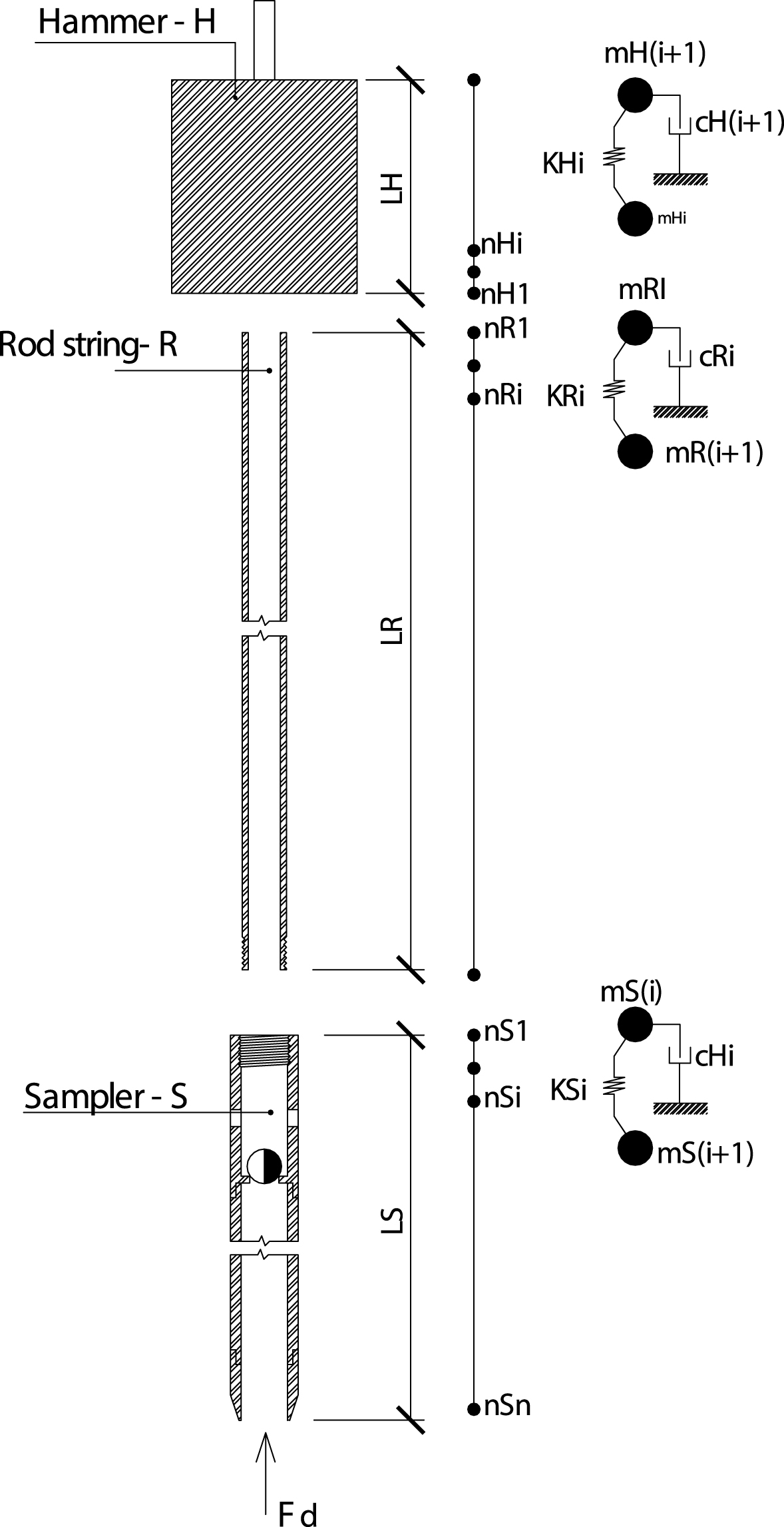
Fig.2
Sampler-soil interaction: (a) reaction mechanism; (b) load-displacemente relationship; (c) reologinal model.
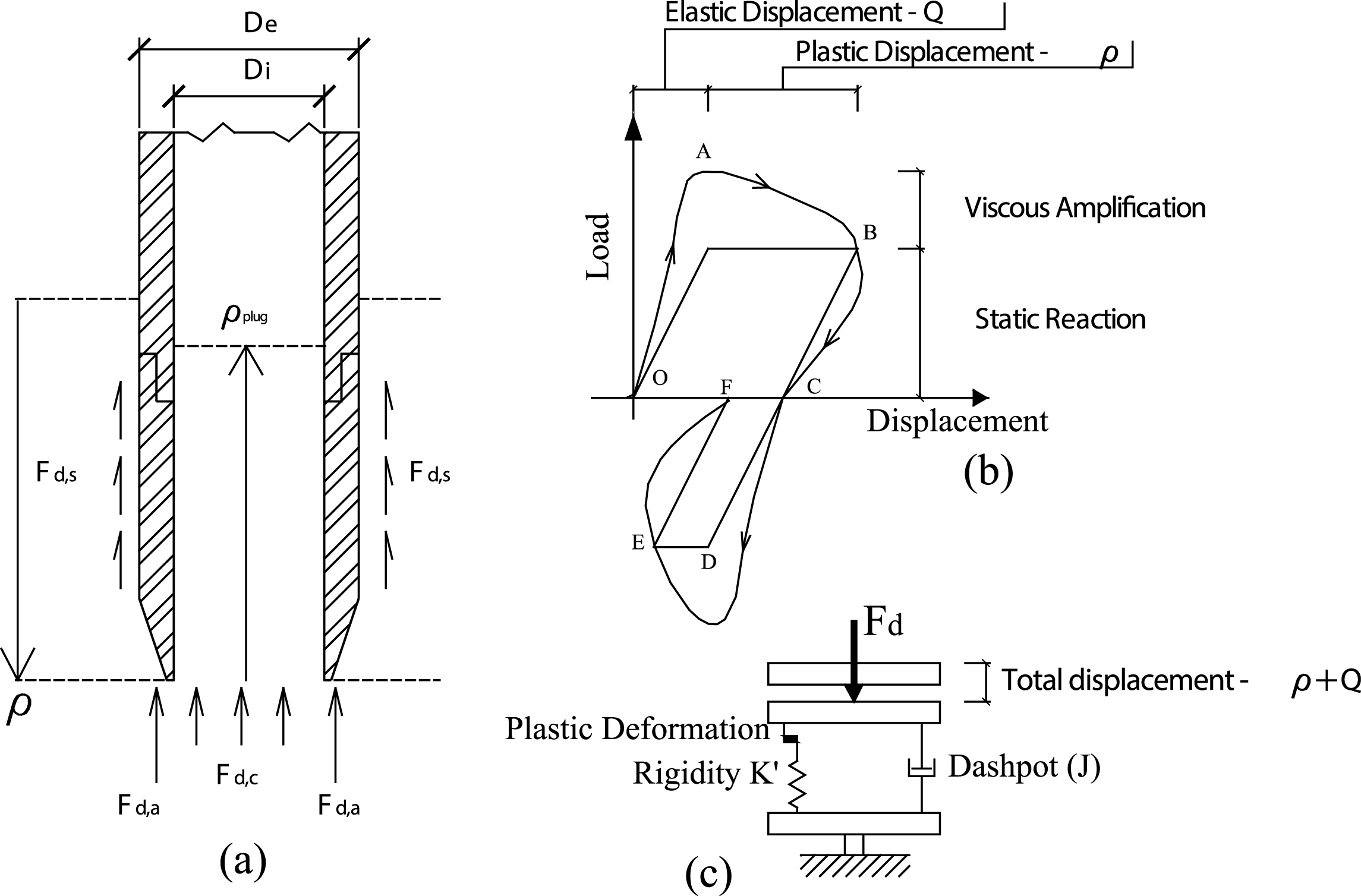
Fig.3
Typical CPTU profile at test site.
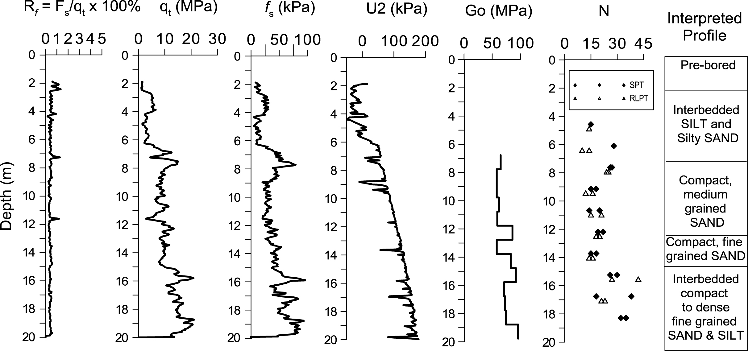
Fig.4
Quasi-static penetration tests performed vs. simulated.
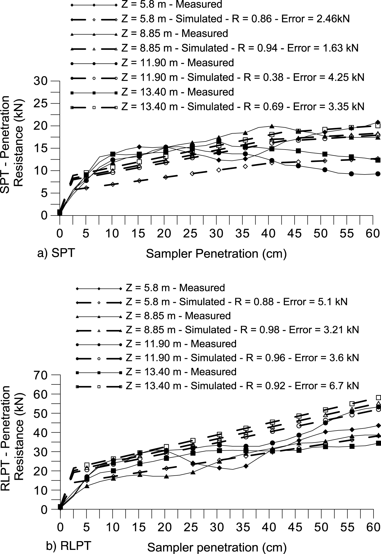
Fig.5
Measured vs. simulated wave signals for SPT and RLPT tests at 7.6 meters depth.
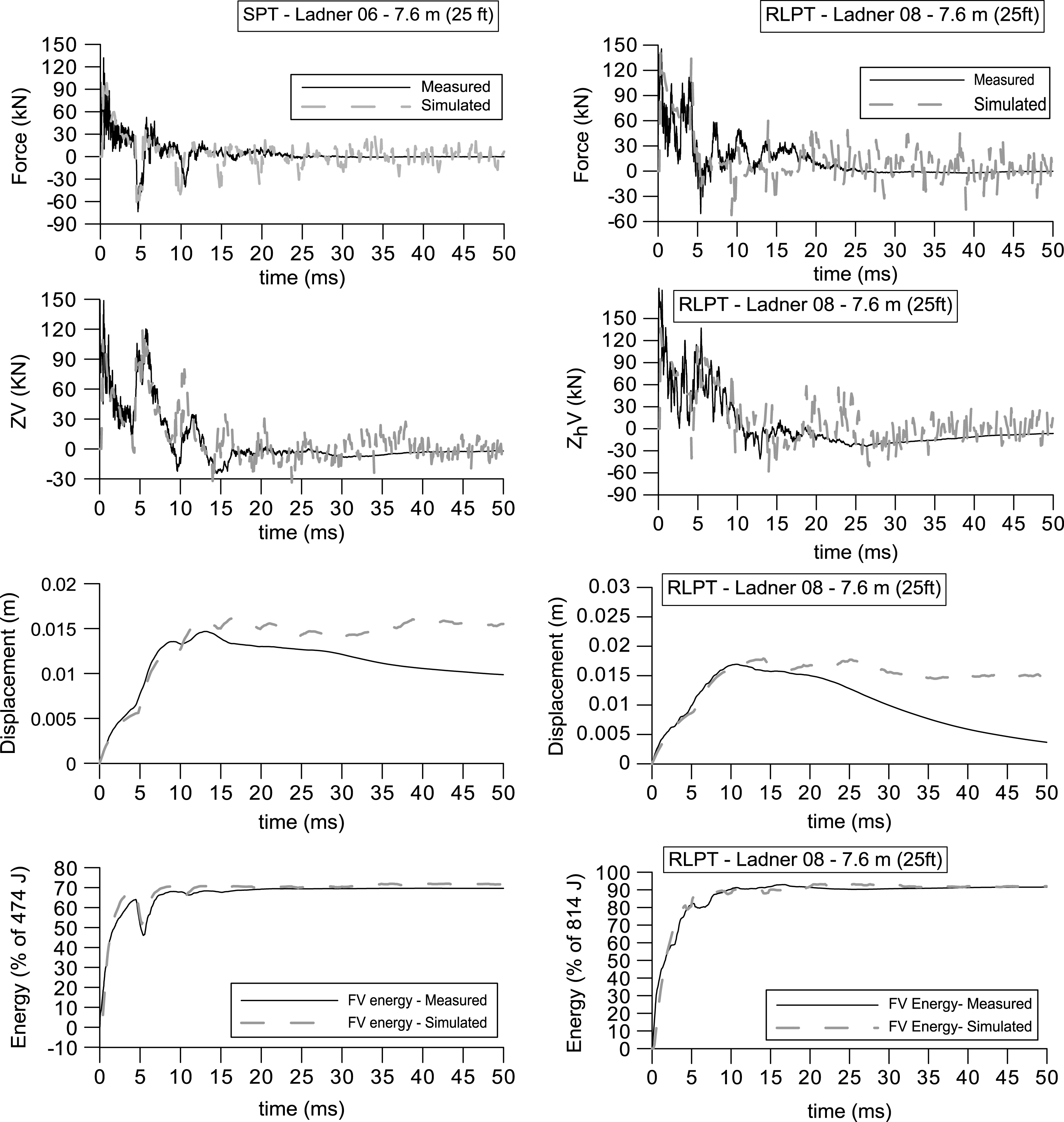
Fig.6
Measured vs. simulated wave signals for SPT and RLPT tests at 18.3 meters depth.
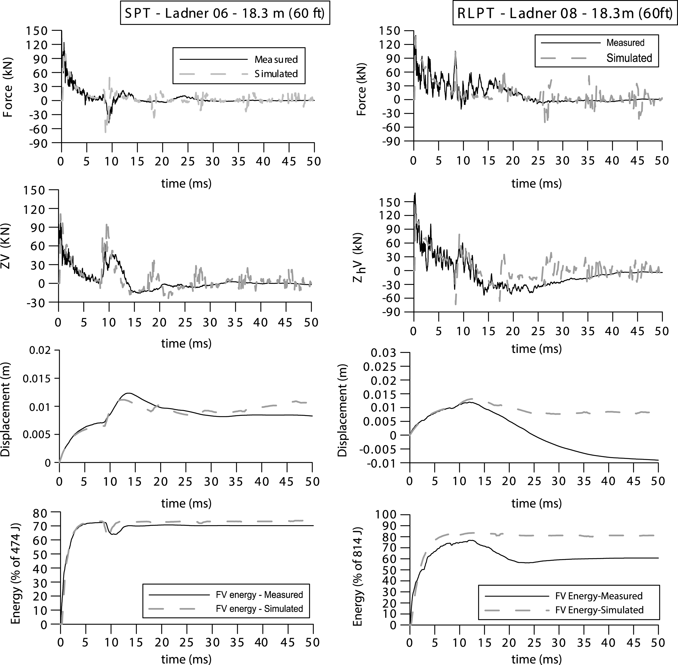
Fig.7
Average penetration per blow measured vs. simulated: SPT and RLPT tests.
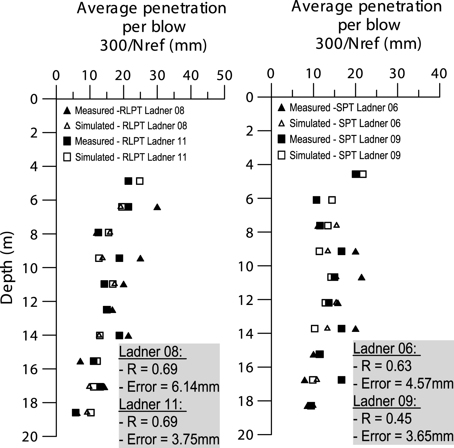
Fig.8
Internal friction angle from SPT, RLP and CPTU.
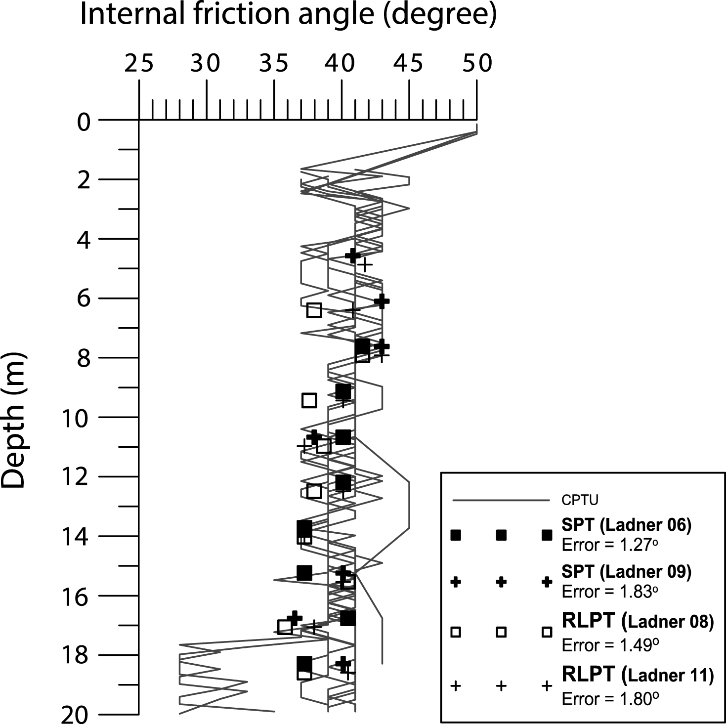
Table 1
Geometrical characteristics of SPT and RLPT tests
| Dynamic penetration test | SPT | RLPT |
| Hammer Type | Safety | Safety |
| Hammer Weight | 63.5 | 136.5 |
| Hammer Drop Height, mm | 762 | 610 |
| Theoretical potential energy, kJ | 474.5 | 816.4 |
| Rod Type | AW | NW |
| Rod Mass (kg/m) | 6.28 | 7.4 |
| Sampler Inner Diameter (mm) | 50.8 | 98.4 |
| Sampler Outer Diameter (mm) | 35.0 | 114.3 |


