
Forest path condition monitoring based on crowd-based trajectory data analysis
Abstract
The development of Road Information Acquisition Systems (RIASs) based on the Mobile Crowdsensing (MCS) paradigm has been widely studied for the last years. In that sense, most of the existing MCS-based RIASs focus on urban road networks and assume a car-based scenario. However, there exist a scarcity of approaches that pay attention to rural and country road networks. In that sense, forest paths are used for a wide range of recreational and sport activities by many different people and they can be also affected by different problems or obstacles blocking them. As a result, this work introduces SAMARITAN, a framework for rural-road network monitoring based on MCS. SAMARITAN analyzes the spatio-temporal trajectories from cyclists extracted from the fitness application Strava so as to uncover potential obstacles in a target road network. The framework has been evaluated in a real-world network of forest paths in the city of Cieza (Spain) showing quite promising results.
1.Introduction
For the last decade, smartphones have been the center of the digital life in modern societies due to their growing popularity. As a result, they are now equipped with several sensors like GPS, accelerometer, microphone, and so forth.
This palette of sensors allows to capture a large amount of contextual information related to the phone’s holders and their surrounding environment [32]. In that sense, this contextual information has been used in several domains like tourism [2], assistance living [23] or personal training [14]. In addition to that, this has eased the development of the mobile crowdsensing (MCS) or human/people sensing paradigm. MCS allows to perceive large-scale phenomena that can not be detected at an individual level like the air pollution levels or the parking state of a city [5].
One of the most useful scenarios where MCS has been used is the deployment of innovative Road Information Acquisition Systems (RIAS). This type of systems report the condition of a road network like longitudinal and lateral roughness, friction, cracking or surface substance. This is instrumental information for road-maintenance operators. Traditionally, this information has been captured by means of infrastructure-based sensors like cameras or high-precision lasers [15]. In that sense, MCS allows to enlarge the coverage of this type of systems beyond the location of the infrastructure-based sensors by using the data captured by the position and motion sensors of the drivers’ handheld devices [16,19,31]. The application domain of this MCS-based solutions restricts itself to urban road networks where different types of motor vehicles travels on [17].
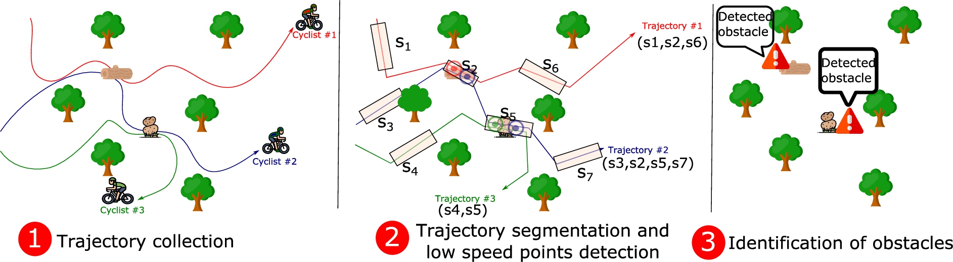
Fig. 1.
Proposed methodology of SAMARITAN. The leftmost figure depicts the collection of the spatio-temporal trajectories of three cyclists moving around the region of interest. The central figure shows the mapping of the captured trajectories a to a set of seven community-based segments (
However, existing literature has payed little attention to other types of road networks that are more common in a country environment like forest paths. These types of roads are widely used by people of all kinds for carrying out a large number of outdoor activities, such as cycling, running or going hiking. For that reason, they may suffer from condition problems that make them difficult to be properly used by visitors, like large obstacles (e.g. fallen trees) or landslides.
Due to their growing popularity, it becomes necessary the development of effective RIASs targeting rural or forest-related road networks. Nevertheless, existing solutions based on infrastructure sensors can not be applied in a cost-effective manner whereas MCS-based solutions rely on sensor-data analyses that focus on detecting fine-grained problems on asphalted roads. Nonetheless, this type of road is not the most common one in many rural environments.
Apart from that, we can also state the growing prominence of fitness apps, like Strava11 or Endomondo22 which operate on a large number of smartphones and wearable devices [25]. These applications allows to endlessly collect different features from exercise activities on large spatial areas. This makes these apps suitable enablers for crowd-based methods in a wide range of domains beyond the smart heath scope [12].
For that reason, the present work introduces SAMARITAN, a system for foreSt pAth Monitoring based on collAboRatIve Trajectory dAta aNalysis. The goal of SAMARITAN is to provide a RIAS for forest paths by following a MCS approach. In particular, it focuses on detecting obstacles that seriously affect the transit of people across such paths like landslides or fallen trunks. To do so, different well-known algorithms from the spatio-temporal trajectory-data mining field have been used.
As Fig. 1 depicts, SAMARITAN firstly collects the spatio-temporal trajectories of cyclists within a region of interest via the fitness-app Strava. Then, a two-level segmentation of the trajectories is applied. This step profits from the segments of interest defined by the own users in the Strava platform. This way, SAMARITAN leverages the knowledge shared by cyclists who move around the monitored spatial region. From the segments extracted of each individual trajectory, a set of candidates where a problem related to the paths state might occur is extracted based on the detection of abnormal stop points. Finally, the candidates extracted at individual level are aggregated to conform the final group of affected segments.
All in all, bearing in mind the open challenges of rural RIAS, the salient contributions of SAMARITAN are the following,
– First of all, it is the first crowd-based RIAS that fully focuses on the rural environment and its particularities.
– Secondly, it makes use of data extracted from a fitness application so as to uncover the state of a road network with great detail. In that sense, such extracted data does not limit to the raw spatio-temporal trajectories from the target users, but also the community-based segments that allow to guide the detection of incidents within the network.
The remainder of the paper is structured as follows. Next, an overview the relevant related work is put forward in Section 2. Section 3 is devoted to describing in detail the logic structure and the processing stages of SAMARITAN. Then, Section 4 discusses the main results of the performed experiments. Finally, the main conclusions and the future work are summed up in Section 5.
2.Related work
In this section we review the most recent advances in MCS-based RAISs along with the usage of data extracted from fitness applications as an enabler of innovative services in different environments.
2.1.MCS-based road information acquisition systems
During the last years, the ubiquity of smart devices carried by drivers has fostered the development of many different approaches for road state monitoring. In that sense, one the first proposals for MCS-based RAIS was put forward in [7]. In this work, authors designed a mechanism able to detect potholes and speedbumps via the analysis of accelerometer and GPS data. In [3] a privacy-preserving mechanism based on fog computing is defined so as to protect the road-condition reports sent by vehicles to the backend servers.
Nevertheless, a common feature of the aforementioned works is that they use onboard devices previously installed on vehicles instead of the drivers’ handheld devices. This seriously limits their feasibility.
As a result, the work in [18] proposed a mechanism that actually profits from a smartphone equipment to detect road-surface problems. However, each device operates independently in the detection task so there is not a real cooperation among users. This makes rather difficult to achieve a complete coverage of a large road network.
This way, in [16] authors proposed an holistic architecture for MCS-based road status monitoring coined CRATER. This mechanism relies on different features extracted from the accelerometer of the users’ smartphones so as to detect patholes and speedbumps via binary classifiers. Another interesting work is [17] where authors made use the crowdsensing platform SmartRoadSense, previously defined in [1], to perform a large-scale deployment of a RAIS as pilot study. Again, an accelerometer stream data is used to detect road-surface roughness. Besides, a time-series approach by means of the well-known algorithm Dynamic Time Warping for the detection of bumps or potholes is described in [28].
Another important research trend goes beyond the detection of single surface problems and intend to provide more general information about the road state. This is the case of [19] where authors follow a similar GPS and accelerometer fusion approach for road monitoring based on MCS. Unlike previous works they provide a more detailed solution to detect the general state of a road, not just surface problems like bumps or potholes. Similarly, a smartphone-based RAIS able to classify the quality of the road surface into five different levels ranging from good to terrible is put forward in [20].
Unlike these works, SAMARITAN focuses on rural roads that do not have the same problems as traditional urban roads. In our case, we detect obstacles that block certain rural paths. For that detection, we do not rely on measurements from the accelerometer sensor of smartphones like in the previous works. Instead of that, we analyze crowd-based GPS traces to detect abnormal stay points that might reflect some problems on certain path segments.
2.2.Analysis of fitness data
During the last years, many different applications have been developed by using the crowd-based data collected by sport and fitness applications.
One of the most interesting fields where this type of data has been applied is the analysis of human mobility flows in cities. For example, fitness-apps data is used in [27] to infer the usage patterns of certain recreational areas whereas in [22] a comprehensive study of mobility patterns based on Strava cycling data in Johannesburg (South Africa) is stated.
Moreover, an analysis based on Strava data of the correlation between certain characteristics of an urban road network and the volume of commute cycling is put forward in [12]. In [13], authors extend this type of analysis by including meteorological data in order to study how weather factors actually affect the behaviour of cyclists. Moreover, the work in [29] correlates the air-pollution level of a city with the mobility patterns of commuting and non-commuting cycling activities by using data from Strava. Similarly, authors in [9] make use of this type of data to detect cycling frequency behaviours in a city and in [10], a data-fusion approach, including data from Strava, is proposed to detect the points of interest where cyclists move within a spatial zone.
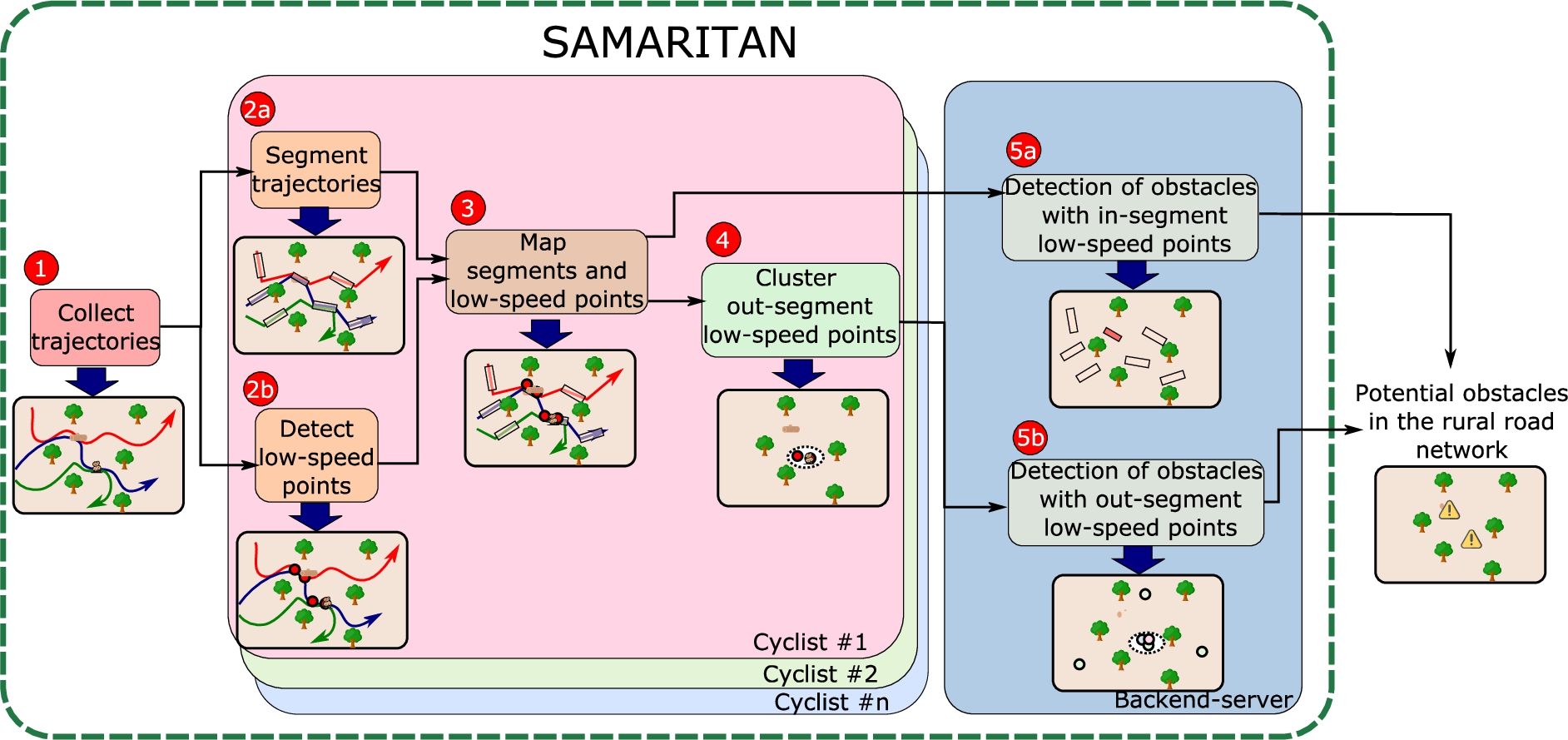
Fig. 2.
Key steps of the SAMARITAN framework. The numbers in red reflect the execution order of each step.
In our work, we use cycling data from Strava in a completely different scope. We make use of the spatio-temporal GPS trajectories extracted from that platform like the aforementioned works. These trajectories represent the routes taken by Strava users. However, we analyze the collected raw trajectories to detect points in a rural road network with potential obstacles. This constitutes a novel usage of this type of fitness data beyond the mobility-pattern extraction mentioned above.
3.The SAMARITAN framework
In this section, we describe in detail the SAMARITAN framework. In that sense, Fig. 2 shows its key steps. As we can see, SAMARITAN follows a crowd-sensing approach where steps 2, 3 and 4 are executed in the contributors’ devices whereas step 5 is executed in a backend server. The following subsections describe in detail each of these steps.
3.1.Collection of the trajectories
The first stage of the framework pipeline focuses on collecting the individual spatio-temporal trajectories of people moving around the target area of interest as Fig. 2 shows. For that goal, we make use of the Application Programming Interface (API) of the Strava platform.
We should remark that SAMARITAN focuses on the trajectories generated by cyclists instead of other sports. The rationale of this filtering is that the detection of problems in the road network is done by the analysis of abnormal speed fluctuations of the incoming trajectories. The cycling trajectories usually have a speed range large enough to perform such an analysis with an acceptable confidence level.
In our scope, a trajectory from a cyclist
Definition 1.
A cyclist trajectory
All the trajectories collected from a particular cyclist c conform the set
3.2.Segmentation of the trajectories
When it comes to analyze spatiotemporal trajectories, one common pre-procesing step is the trajectory segmentation [34]. This consists of dividing a trajectory into fragments by several criteria like time interval, spatial shape, semantic meaning. This allows to compress the incoming trajectory in a more simple format.
For this step, SAMARITAN makes use of the segments
Since each segment
As a result of this join, a new segment-based trajectory
Definition 2.
A cyclist segment-trajectory
For example, in Fig. 1, the trajectory of cyclist 1,
3.3.Detection of low-speed points
Apart from the segmentation described above, we also analyze each incoming raw trajectory
The rationale of detecting these low-speed parts of a trajectory is that they might indicate the presence of certain obstacles during a cyclist’s trip. In these points, a cyclist usually needs to slow down and, in some cases, even get off his bike. This is reflected as a sudden drop in the speed profile of the trajectory. These low-speed points can be regarded as outliers in the speed time-series of a trajectory.
This speed time-series can be calculated from the sequence of timestamped points of a raw trajectory stated in Def. 2. In particular, for each pair of consecutive points
Definition 3.
A cyclist trajectory speed profile
In order to detect the outliers from this profile, SAMARITAN makes applies the Generalized Extreme Student Deviation (GESD) test over the time-series
In order to only retain the low-speed outliers, we discard those abnormal values that are above 0.5 m/s. As a result of this process, a set of abnormally low speed values
Finally, we map each abnormal speed
It is worth-mentioning that the aforementioned procedure relies on GPS trajectories that are defined at a very fine granularity where the current location of the cyclist is captured every few seconds. The functionality of SAMARITAN would be rather limited if the GPS feed (e.g. the cyclist’s smartphone or smartwatch) was configured with a large sampling rate because, in that case, some low-speed points might not be detected.
However, high-intensity sports are better monitored when high sampling rates above 10 Hz are used [24]. Furthermore, some manufacturers of GPS trackers in the sport field actually recommend a similar configuration for their devices [30]. Consequently, it is sensible to expect that the potential contributors of SAMARITAN would generate fine-grained trajectories during its cycling activities in most of the cases.
3.4.Mapping of low-speed points and segments
Once we have uncovered the abnormal low-speed points of a trajectory, we need to detect whether these points occurred or not in any of the community-based segments of the trajectory. This is because SAMARITAN handles the points in a different manner depending on they fit or not into a Strava segment as we will see later.
Consequently, this step of SAMARITAN takes as input the Strava segments
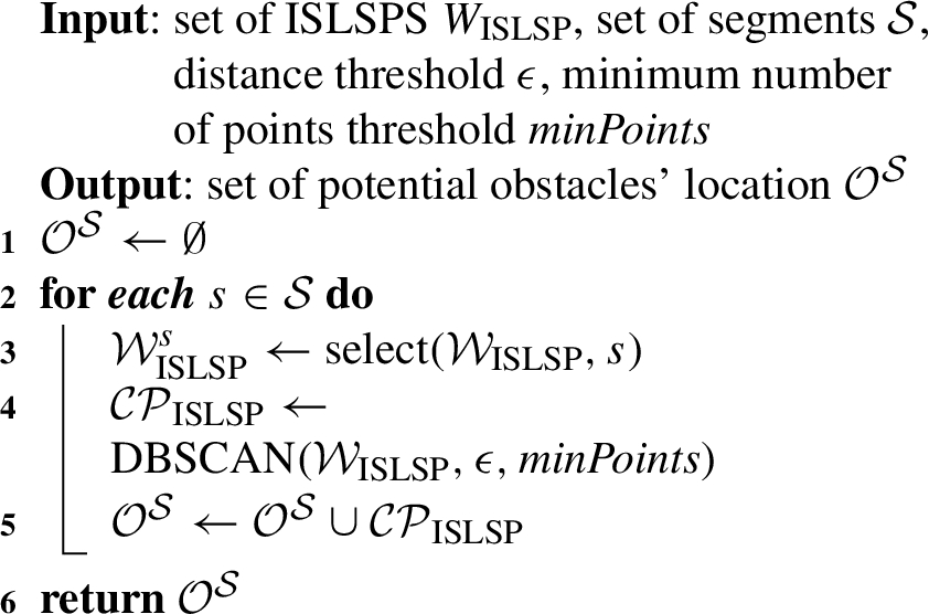
Algorithm 1:
Pseudo-code of the low-speed points mapping
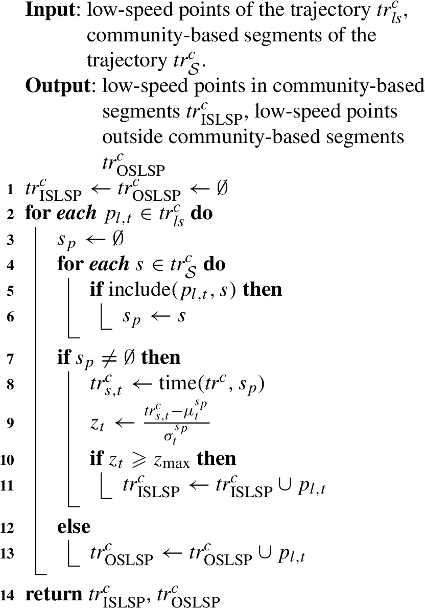
As we can see from the pseudo-code, we just take each low-speed point in
If the point fits into a segment then we perform a time-based analysis (lines 7–11 of Alg. 1). The idea of this analysis is that if a cyclist had to abruptly slow down one or more times within a segment then the time required to cover that segment would be meaningfully larger than the cyclist’s average for that particular segment. Otherwise, the detected low-speed points may be just noisy measurements.
To do so, we profit from a feature of the Strava API44 that allows to extract the historic time records of a cyclist for a given segment. Hence, we can compute the mean and the standard deviation of these time records for a cyclist c in any segment
Apart from that, we can calculate the actual time required by a cyclist to cover a segment s during a trajectory
If this z-score is above a certain threshold (
Otherwise, if the low-speed point does not fit into any segment we can not perform the aforementioned time analysis. This type of out-segment points are handled in a different manner. Thus, they are included in the complementary set of out-segment low-speed points (OSLSPs)
–
–
Finally, these two sets are processed in a different way by SAMARITAN. This is because both sets represent completely different situations. Whilst the low-speed points in
3.5.Clustering of the out-segment low-speed points (OSLSPs)
As we have mentioned before,
In this case, we need to determine if these abrupt decelerations correspond to recent changes in the mobility behaviour of cyclist c or they are just part of his usual behaviour. This because a sudden change in the mobility profile of a cyclist in terms of new stop points might indicate the presence of recent obstacles in these points.
In order to determine if the OSLSPs are part of the usual mobility behavior of a cyclist or not, we follow a density-based clustering approach based on the well-known DBSCAN algorithm [8]. This way, we collect all the OSLSPs from each cyclist c during the last
Based on the OSLSPs included in that dataset, we applied the procedure described in Algorithm 2. First of all, we apply the density-based clustering algorithm DBSCAN [8] to
– For each OSLSP
– If the number of points within that neighborhood is above the
The set of centroids obtained from this algorithm (
Algorithm 2:
Pseudo-code of OSLSPs clustering
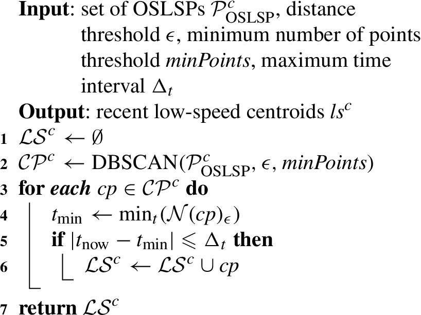
To do so, we extract the minimum timestamp
An illustrative example of this process is shown in Fig. 3. In this scenario, six different trajectories from the same cyclist c are collected, each one comprising a single OSLSP. Next, SAMARITAN executes Algorithm 2. In this case,
Fig. 3.
Example of detection of a r-OSLSP
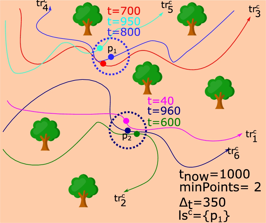
A similar situation arises with trajectory
As Fig. 2 depicts, we should mention that the four procedures described in Sections 3.2 to 3.5 are executed independently for each cyclist in
At this point, we should indicate that it is true that GPS trajectories usually suffer from some inaccuracies due to signal-reception problems. They might cause that the path represented by a trajectory does not completely fit the actual path followed by the moving object. However, this type of error usually arises in scenarios where signal occlusion occurs like indoor environments or certain urban regions [33].
In that sense, the present framework focuses on an outdoor scenario that may reduce the incidence of this type of error. Moreover, the low-speed point extraction does not rely on the actual trace followed by a cyclist but on his speed evolution. It is true that inaccurate GPS trajectories might cause the system to wrongly infer false low-speed points or not to detect certain true ones. However, the inference of ISLSPs and OSLSPs depends on the latent speed of a trajectory at Strava segment level (for ISLSPs) or considering a ϵ-neighborhood (for OSLSPs). This segment or cluster matching procedure is similar to the map-matching step performed by many solutions for GPS trajectory processing in the urban and vehicular environment [4,6,21]. This allows to reduce the impact of these noisy points in the speed pattern of a trajectory. Hence, this makes it possible to detect that a cyclist has moved abnormally slow or not.
Finally, the
3.6.Detection of obstacles with in-segment low-speed points (ISLSPs)
Based on the procedure described in Section 3.4, the client-side of SAMARITAN was able to extract the set
To do so, SAMARITAN follows a batch-based analysis (depicted as step 5a in Fig. 2). To begin with, it defines a time-based sliding window that collects all the sets
Given the aforementioned dataset, SAMARITAN detects changes in the mobility behavior within each Strava segment by following the procedure described in Algorithm 3.
Algorithm 3:
Pseudo-code of the detection of potential obstacles based on ISLSPs
Basically, we select for each segment
An alternative approach for this step would have been the execution of a global instance of DBSCAN independent of any segment. Nonetheless, this had merged together ISLSPs of different segments. Since each Strava segment conceptually represents a particular road slice with different features it is necessary to analyze each segment independently.
All in all, we can see that the Strava segments provides a sparse spatial tessellation of the area under study. They allow to group together stop-points in spatial areas frequently crossed by cyclists.
3.7.Detection of obstacles with out-segment low-speed points (OSLSPs)
In Section 3.5 we put forward how uncover the r-OSLSPs from each cyclist under control. Therefore, we can use that information so as to detect a new set of obstacles apart from the ones uncovered by the procedure described in the previous section based on ISLSPs.
As in Section 3.6, we analyze the collected r-OSLSPs by making use of a batch-based approach. In particular, we gather the r-OSLSPs from all the cyclist in
Next, each time
The resulting set of centroids indicate spatial regions (not covered by a Strava segment) where several cyclist had to abruptly decelerate during, at least, the last
We can see that, in order to process, the OSLSPs SAMARITAN follows a two-level DBSCAN clustering.
– In the first level, OSLSPs are clustered together for each individual cyclist as put forward in Section 3.5.
– In the second level, all the r-OSLSPs extracted in the first clustering level are aggregated and clustered again so as to come up with the final set of candidate locations of obstacles (
This approach makes SAMARITAN able to be adapted to a client-server infrastructure where the first clustering level is executed in the cyclists’s personal devices whereas the second one is executed in a back-end server with the meaningful stops from the contributors.
Finally, the set of obstacles
3.8.Summary of the SAMARITAN pipeline
For the sake of clarity, here we sum up the key steps that compose the processing pipeline of the SAMARITAN framework as shown in Fig. 2.
First of all, the client-side SAMARITAN collects the spatio-temporal trajectories of its target cyclist moving around the spatial area under monitoring (step 1 in Fig. 2). Then, these trajectories are split based on the community-defined Strava segments and their low-speed points are uncovered (steps 2a and 2b). Next, these low-speed points are mapped based on the Strava segments (step 3). This gives raise to OSLSPs and ISLSPs. After that, the OSLSP are clustered so as to uncover the r-OSLSPs (step 4).
Finally, the central server of the framework merges together the ISLSP in each Strava segment to detect the potential obstacles within these segments (step 5a). At the same time, the r-OSLSPs are clustered with DBSCAN to identify regions with potential obstacles located outside any Strava segment (step 5b).
3.9.Data privacy aspects of SAMARITAN
Regarding the issues about the cyclists’ privacy when using SAMARITAN, it is true that the proposed solution relies on the analysis of the spatio-temporal trajectories from cyclists so as to detect forest-path incidents. However, the initial processing of the raw GPS traces is performed locally in the client side of the framework running in each cyclist’s mobile device. This client side only sends to the central server the low-speed points
Consequently, the location data sent to the central server is actually quite limited. In addition to that, the server only needs to store the low-speed points sent by the cyclist during a certain amount of time due to its batch-based computation of the aggregated points (see Sections 3.6 and 3.7). After
For the sake of completeness, the privacy-preserving solution stated in [3] focuses on a scenario where vehicles are endlessly reporting real-time data to certain intermediate entities called Roadside Units (RSUs). These units analyze the fine-grained data from vehicles and report possible alerts about road conditions to upper cloud servers. Authors focus on developing a mechanism to secure the communication channel between vehicles and RSUs as a large amount of private data flows through it. On the contrary, SAMARITAN does not require contributors to send real-time data to a central or intermediary server but certain candidate points where a road problem might occur. Therefore, the direct integration of the aforementioned privacy solution in SAMARITAN would not be possible.
3.10.Configuration of SAMARITAN
The proposed framework is able to control its sensibility to detect forest-path problems. This is because this detection mainly depends on two different sets of parameters, the lengths of the time-windows (
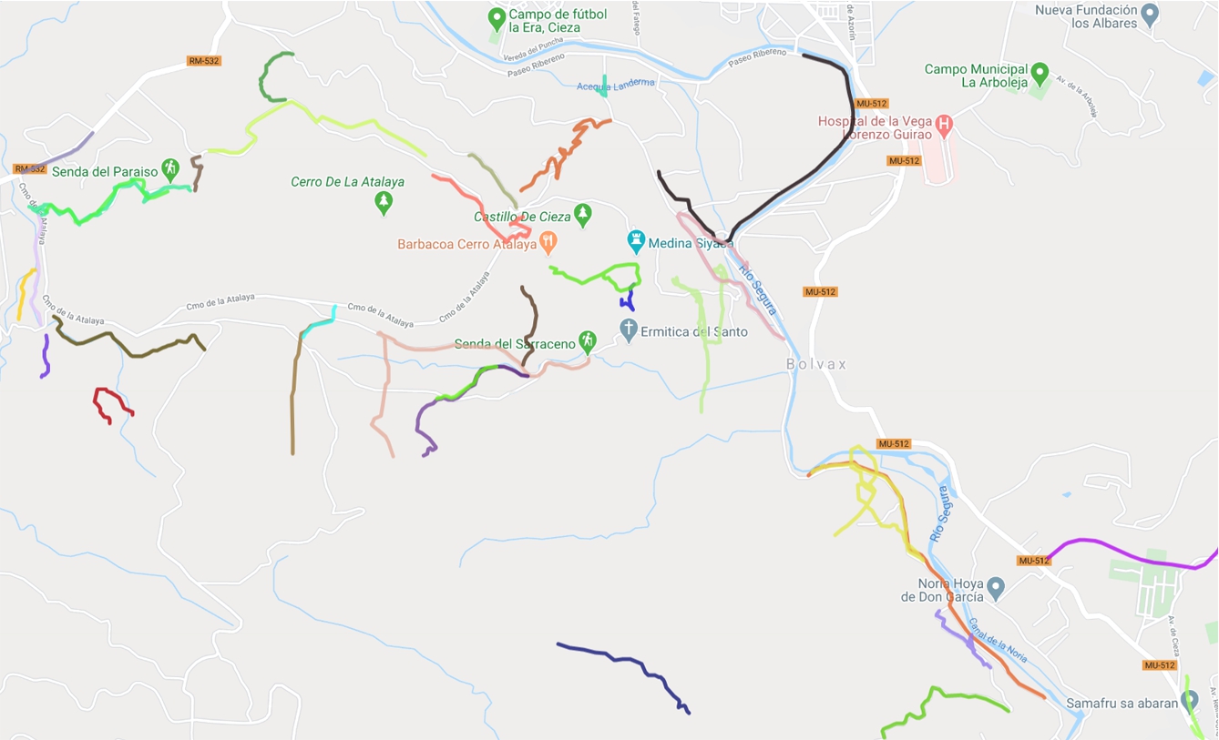
Fig. 4.
Spatial location of the Strava segments used in the evaluation. Each segment is depicted as a coloured line.
These sets of parameters allow to adjust the behaviour of SAMARITAN with respect to the number of available cyclists using the service. Depending on the number of contributors, the SAMARITAN administrator can reduce or increase the length of the time windows by considering the storage capability of the central server.
In case of the number of contributors is high, the length of the time-windows can be reduced. This is because provided that there is a problem in a forest-path many cyclists would report abnormal low-speed points in a short period of time.
On the contrary, if the number of contributors is low, the administrator can reduce the density-parameters of the DBSCAN algorithm so as to increase the sensibility of the solution. It is true that this might lead to reporting some false positives but, in this case, the important goal is to detect as many obstacles as possible.
4.Evaluation of the framework
We have evaluated SAMARITAN in the city of Cieza at the southwest of Spain. This small city is surrounded by many forest paths that are very popular among local cyclists. Furthermore, the region was heavily affected by a cold front in September of 2019.55 This caused a lot of damage to the roads in the area.
In order to apply SAMARITAN in that region we focused on the city outskirts included the spatial bounding box defined by the latitude-longitude coordinates
4.1.Data description
The details of three datasets used for the present evalution are described next.
4.1.1.Strava segments under consideration
The target geographical area includes 36 Strava segments whose spatial distribution within the target bounding box is shown in Fig. 4. As we can see, these segments are not homogeneously distributed in the target area. This is because they are defined by the own Strava users. Therefore, they usually represent parts of the road that are interesting or event challenging for the cyclist perspective.
Besides, Table 1 indicates the minimum, average and maximum length of these segments. We can see that these segments cover a wide range of lengths from a few meters to almost 2000 meters.
Table 1
Length parameters of the Strava segments
| Segment feature | Value |
| Min. segment length | 92 m |
| Max. segment length | 1922 m |
| Avg. segment length | 673 m |
| Total segment length | 24228 m |
Fig. 5.
Histogram with the length distribution of the Strava segments. The x-axis shows the segment length and the y-axis indicate the number of segments. The red line shows the cumulative percentage of segments.
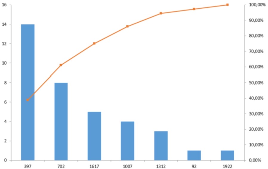
Fig. 6.
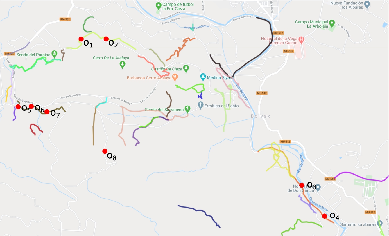
Location of the eight target obstacles. Each obstacle is depicted as a red point. Obstacles
Furthermore, Fig. 5 shows the length distribution among the collected Strava segments. From this distribution, we can see that most of the segments cover road parts of roughtly 317 meters.
This variety of lengths justifies the step take by SAMARITAN to identify obstacles within Strava segments described in Section 3.6. As we saw in that section, the ISLSPs of a particular segment are clustered by means of DBSCAN. This allows to cope with quite large segments as the framework is able to provide different tentative locations within a segment.
4.1.2.Spatio-temporal trajectories under study
Regarding the trajectories used as input by the framework, we have collected the data from 5 different cyclists during a six-month period from 01/06/2019 to 31/12/2019. This has given raise to 98 different spatio-temporal trajectories. The sampling rate of these trajectories varied from 1 s to 3 s.
4.1.3.Target obstacles
In order to test the accuracy of SAMARITAN, eight particular locations within the target geographical area where a clear alteration of a forest path occurred were used as ground truth. They were identified as
All these obstacles were caused by a three-day cold front that occurred during the 11st and 14th of September of 2019 in the southeast of Spain. This storm caused torrential downpours that seriously affected the spatial region considered by the use case. As a result, five of the target problems were caused by landslides, three by fallen trees and one by a broken pipe. All these obstacles were manually discovered by the authors during a three-day campaign from 27th to 29th of September. In that sense, this ground-truth information was not revealed to the 5 cyclists acting as contributors of SAMARITAN.
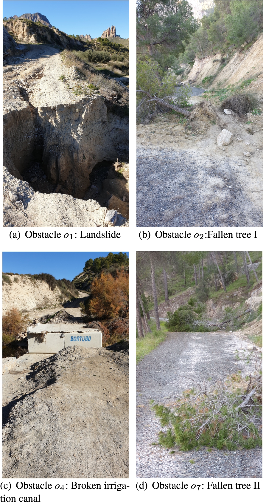
For the sake of clarity, Table 2 shows the relationship between the aforementioned obstacles and some detail of the segments comprising them. Furthermore, Fig. 7 shows some of these obstacles. As we can see, they were caused by landslides (obstacle
Table 2
Distribution of the in-segment target obstacles. The segment name column indicates the name of the segment according to the Strava API
| Segment name | Segment length | Obstacle id. |
| Bajada Senda del Moro ( | 1500 m | |
| Menu-Puente Abaram ( | 1900 m | |
| Subida Camino-Viejo ( | 1100 m | |
Fig. 7.
Visual inspection of the detected obstacles.
4.2.Framework parameters
For the sake of clarity, Table 3 sums up the parameter settings in this use case.
As we can see, the parameters that define the time periods to analyze the low-speed points (
Table 3
SAMARITAN settings
| Parameter | Step | Value |
| Low-speed points mapping (Section 3.4) | 1.5 | |
| ϵ | OSLSP clustering (Section 3.5) | 250 m |
| minPoints | 2 | |
| 720 h | ||
| 360 h | ||
| Obstacle detection with ISLSPs (Section 3.6) | 360 h | |
| 4 | ||
| Obstacle detection with r-OSLSPs (Section 3.7) | 360 h |
This is because SAMARITAN relies on routes made by cyclist during their free time, so they can not be regarded as daily trips. This makes the required time periods to process data quite large.
4.3.Analysis of the results
Given the trajectories and segments described above, SAMARITAN reported 10 different potential obstacles
Fig. 8.
Location of the ten obstacles detected by SAMARITAN. Each obstacle is depicted as a red point whereas the true obstacles are shown in green.
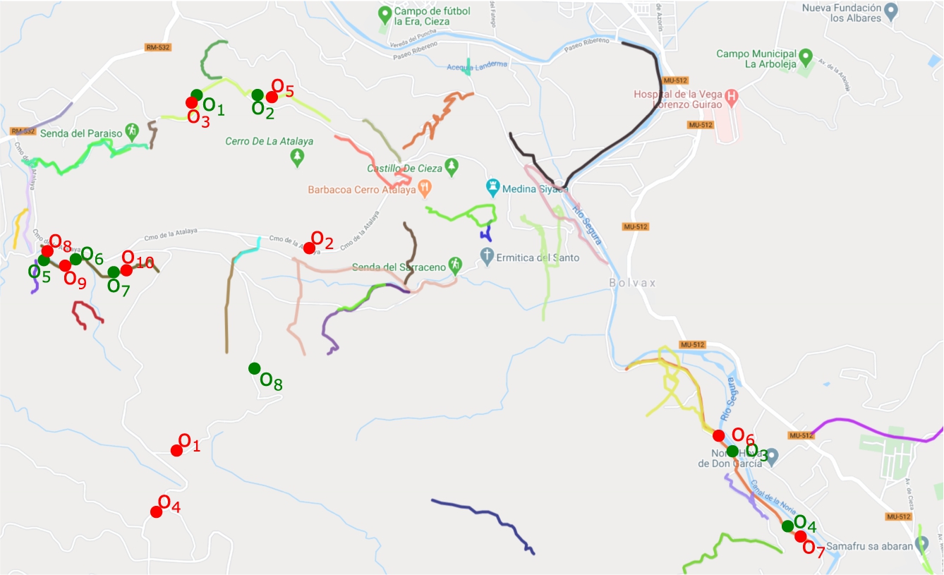
From this set, seven of them (
Table 4
Relation between the inferred obstacles by SAMARITAN and the true ones along with the distance between each pair of inferred and true points. The rows in grey indicate distances below 150 m
| Inferred obstacle | Closest true obstacle | Distance |
| 1133 m | ||
| 1344 m | ||
| 65 m | ||
| 1500 m | ||
| 87 m | ||
| 81 m | ||
| 130 m | ||
| 37 m | ||
| 26 m | ||
| 91 m |
In order to properly analyze these results, we study the speed behaviour of the trajectories in the three segments comprising seven of the true obstacles (
Furthermore, some of these obstacles were repaired by authorities during the time period of the present use case. This allowed us to split such speed profile in three different time intervals, 1) one including the trajectories before the occurrence of the obstacle event, 2) another including the trajectories in the time interval during which the obstacle was present and 3) a final time interval covering the trajectories after the forest-path problem was solved.
To set the date thresholds defining each interval, we used the average time marks of the five target cyclist in each segment depicted in Fig. 9. As we can see, there is a clear increment of the time marks in the three segments after the 8th of September of 2019. This consistent with the dates of the cold front affecting the region in that month.
After that, the marks behavior varies depending on the segment. In segment
Fig. 9.
Time marks of the cyclists in segments
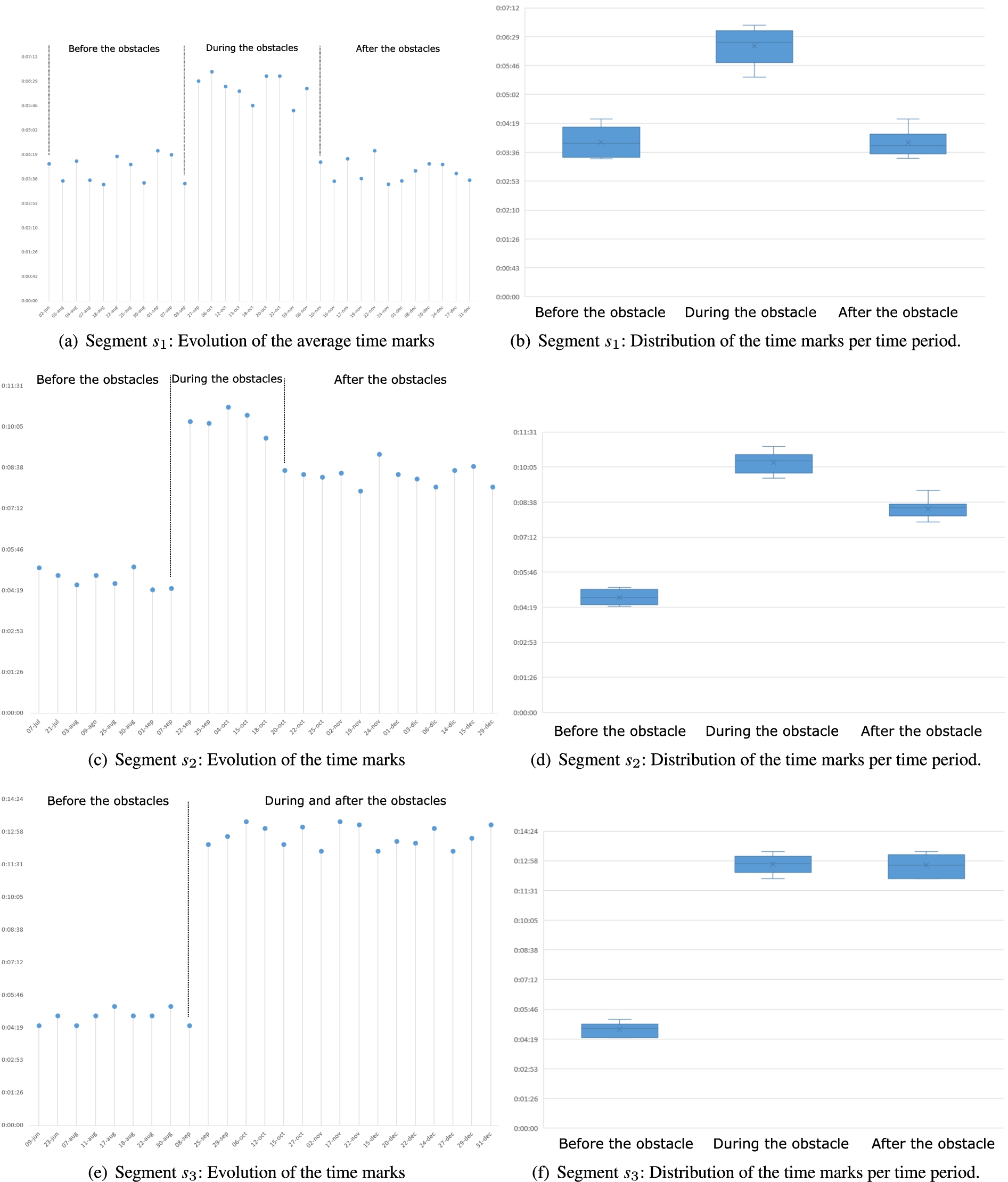
Besides, the speed distributions shown in Figs 9b,d&f confirm that the presence of obstacles clearly affects the speed behaviour of cyclists around the affected region.
Figure 10 shows the average speed evolution of the target trajectories in segments
Fig. 10.
Average speed evolution of the trajectories for segments
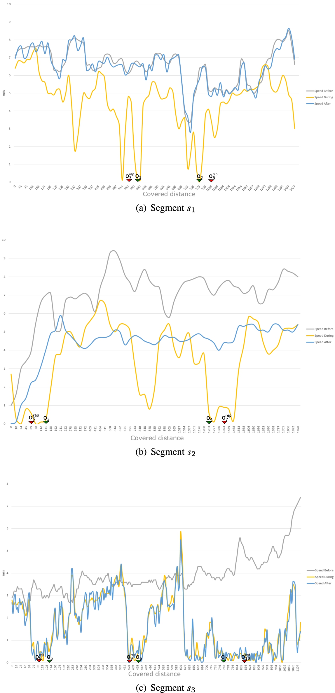
The first thing to note is that there is a clear difference between the trajectories’ speed profile depending on the time period. This shows that the presence of obstacles meaningfully affects the mobility flows of cyclist moving around the area under control.
More in detail, we can see that the speed-profile after the obstacle events and before their repair are quite similar in segment
If we focus on the speed behavior of the trajectories during the obstacle presence (yellow lines in Fig. 10), we can clearly see a set of sudden speed drops around the obstacles location. This generates different ISLSPs from the trajectories moving along these segments. This allows to detect obstacles
However, obstacle
Finally, SAMARITAN was not able to detect the true obstacle
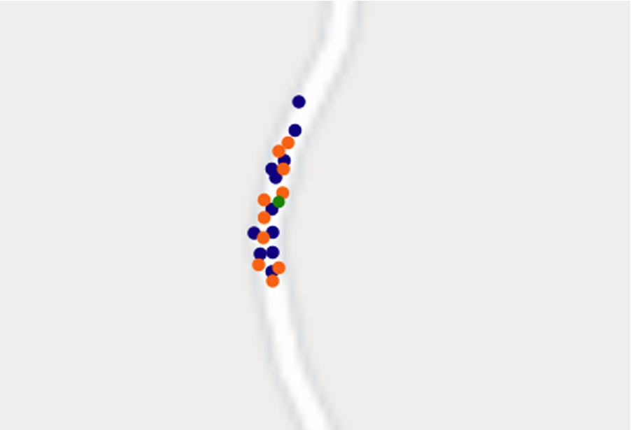
Fig. 11.
Location of all the OSLSPs generated during the experiment around obstacle
4.4.Lessons learnt
From this use case we can draw up some interesting findings.
First of all, SAMARITAN uses two types of crowdsensing data to detect forest-path problems, an internal and an external one. The former is the GPS trajectories generated by the cyclists acting as contributors that are explicitly processed by the client side of the framework. The latter is the road-segment statistics gathered from a third-party community service like Strava. In that sense, the use case has shown that the enrichment of a MCS architecture with crowd-based data from an external platform is a promising approach to extend the usage of these architectures to new domains such as the detection of road problems in rural regions.
Secondly, the evaluation of the framework has proved that, as many MCS architectures, the reliability and accuracy of the proposed solution strongly depends on the density of contributors. In that sense, road problems occurring within Strava segments are more likely to be discovered. This is because these segments are defined by the Strava users in parts of the road network covered by a large number of cyclists. This limitation is a side effect of relying on Strava as an input source.
However, this dependence allows SAMARITAN to leverage the data shared by users in Strava. As a result, it avoids a cold-start problem when it comes to retrieve historic speed-behaviour of cyclists of the segments in each new deployment. In that sense, if the Strava platform disappeared or restricted its access via API then it would be necessary to find an alternative public feed providing historic data about cyclist mobility in the target areas. In that sense, some spatial repositories, like OpenStreetMap, allows users to upload their own GPS trajectories.66 Another possible alternative would be the composition of the segment statistics directly by SAMARITAN. This could be done in an incremental manner as long as the system processes data from the contributors. However, this option would suffer from the same cold-start problem described above.
Finally, the crowd-based approach followed by SAMARITAN to collect fitness-related data limits its application to scenarios accomplishing certain requirements. Since the system relies on sudden and abrupt deceleration of the cyclists as initial step to fire the path-problem detection mechanism, SAMARITAN would not be a feasible solution in urban environments where cyclists usually face many different obstacles (e.g traffic lights, pedestrians and so forth) that may make them to abruptly stop. This would generate plenty of noisy data and the system would report a large number of false positives.
5.Conclusions
The endless enrichment of personal mobile contrivances with new sensing capabilities has enabled the development of many collaborative applications. In this context, MCS-based RIASs allow to monitor the state of large portions of a road network in a cost-effective manner. However, existing solutions focus on a rather limited scope as they assume that devices providing sensor data are used by car drivers.
In this context, the present work introduces SAMARITAN, a MCS-based RIAS that targets forest paths. This type of roads are very popular to do many different sports like cycling or hiking. However, they can also suffer from problems that affect their usual transit flow. These problems are caused by the presence of obstacles like fallen trees or landslides.
SAMARITAN profits from the growing popularity of fitness Internet applications to perform its path-monitoring task. In particular, it makes use of cyclist trajectories and community-based segments collected from Strava, a foremost sport application. The evaluation of the framework in a real-world scenario has shown that our solution has been able to accurately detect most of the target obstacles. However, as most solutions based on the MCS paradigm, its reliability depends on the density of contributors in the target area.
The key benefit of SAMARITAN with respect to other possible alternatives for forest-path monitoring is that it follows an opportunistic MCS approach. As a result, contributors do not need to explicitly notify the locations of the forest-path incidents because the system is able to do that based on their automatically-generated GPS trajectories. In that sense, potential alternatives where users must explicitly report the problems that they see in the paths would suffer from large usability problems. The most important one is that this type of approach would require users to stop halfway through their sport activity every time they spot an incident, report the problem and lastly resume their training. This would discourage the usage of these type of alternatives by many different potential contributors within the fitness field.
All in all, the present work would help rural administrations to better maintain their forest paths networks. It would allow these authorities to control large geographical areas at affordable cost provided that they are visited by enough cyclists.
Finally, future work will extend the framework to consider other contextual factors for obstacles detection. This way, the current weather conditions or the orography of the target region under study might be relevant features in order to asses whether an abnormal stop is caused by a road-condition problem or not.
Notes
Acknowledgements
Authors would like to thank the cyclists who kindly collaborated in the evaluation of the tool by giving up their GPS trajectories. Moreover, this work has been supported by the Fundación Séneca del Centro de Coordinación de la Investigación de la Región de Murcia under Project 20813/PI/18, and by the Spanish Ministry of Science, Innovation and Universities under grant RTC-2017-6389-5.
References
[1] | G. Alessandroni, L. Klopfenstein, S. Delpriori, M. Dromedari, G. Luchetti, B. Paolini, A. Seraghiti, E. Lattanzi, V. Freschi, A. Carini et al., Smartroadsense: Collaborative road surface condition monitoring, in: Proceedings of the UBICOMM, (2014) , pp. 210–215. |
[2] | I. Ayala, L. Mandow, M. Amor and L. Fuentes, A mobile and interactive multiobjective urban tourist route planning system, Journal of Ambient Intelligence and Smart Environments 9: (1) ((2017) ), 129–144. doi:10.3233/AIS-160413. |
[3] | S. Basudan, X. Lin and K. Sankaranarayanan, A privacy-preserving vehicular crowdsensing-based road surface condition monitoring system using fog computing, IEEE Internet of Things Journal 4: (3) ((2017) ), 772–782. doi:10.1109/JIOT.2017.2666783. |
[4] | L. Bayındır, A survey of people-centric sensing studies utilizing mobile phone sensors, Journal of Ambient Intelligence and Smart Environments 9: (4) ((2017) ), 421–448. doi:10.3233/AIS-170446. |
[5] | C. Borcea, M. Talasila and R. Curtmola, Mobile Crowdsensing, CRC Press, (2016) . |
[6] | C. Chen, Y. Ding, X. Xie, S. Zhang, Z. Wang and L. Feng, TrajCompressor: An online map-matching-based trajectory compression framework leveraging vehicle heading direction and change, IEEE Transactions on Intelligent Transportation Systems 21: (5) ((2020) ), 2012–2028. doi:10.1109/TITS.2019.2910591. |
[7] | J. Eriksson, L. Girod, B. Hull, R. Newton, S. Madden and H. Balakrishnan, The pothole patrol: Using a mobile sensor network for road surface monitoring, in: Proceedings of the 6th International Conference on Mobile Systems, Applications, and Services, MobiSys’08, Association for Computing Machinery, New York, NY, USA, (2008) , pp. 29–39. ISBN 9781605581392. doi:10.1145/1378600.1378605. |
[8] | M. Ester, A density-based algorithm for discovering clusters in large spatial databases with noise, in: Proc. 2nd Int. Conf. on Knowledge Discovery and Data Mining, AAAI Press, Portland, Oregon, (1996) . |
[9] | G. Griffin, K. Nordback, T. Götschi, E. Stolz and S. Kothuri, Transportation research circular E-C183: Monitoring bicyclist and pedestrian travel and behavior: Current research and practice, Transportation Research Board of the National Academies, Washington, DC, 2014. |
[10] | G.P. Griffin and J. Jiao, Where does bicycling for health happen? Analysing volunteered geographic information through place and plexus, Journal of Transport & Health 2: (2) ((2015) ), 238–247, http://www.sciencedirect.com/science/article/pii/S2214140514001042. doi:10.1016/j.jth.2014.12.001. |
[11] | F.E. Grubbs, Procedures for detecting outlying observations in samples, Technometrics 11: (1) ((1969) ), 1–21. doi:10.1080/00401706.1969.10490657. |
[12] | H.H. Hochmair, E. Bardin and A. Ahmouda, Estimating bicycle trip volume for Miami-Dade county from Strava tracking data, Journal of Transport Geography 75: ((2019) ), 58–69, http://www.sciencedirect.com/science/article/pii/S0966692318308639. doi:10.1016/j.jtrangeo.2019.01.013. |
[13] | J. Hong, D.P. McArthur and J.L. Stewart, Can providing safe cycling infrastructure encourage people to cycle more when it rains? The use of crowdsourced cycling data (Strava), Transportation Research Part A: Policy and Practice 133: ((2020) ), 109–121. |
[14] | V. Janko, B. Cvetković, A. Gradišek, M. Luštrek, B. Štrumbelj and T. Kajtna, e-Gibalec: Mobile application to monitor and encourage physical activity in schoolchildren, Journal of Ambient Intelligence and Smart Environments 9: (5) ((2017) ), 595–609. doi:10.3233/AIS-170453. |
[15] | P. Jonsson, J. Casselgren and B. Thörnberg, Road surface status classification using spectral analysis of NIR camera images, IEEE Sensors Journal 15: (3) ((2015) ), 1641–1656. doi:10.1109/JSEN.2014.2364854. |
[16] | F. Kalim, J.P. Jeong and M.U. Ilyas, CRATER: A crowd sensing application to estimate road conditions, IEEE Access 4: ((2016) ), 8317–8326. doi:10.1109/ACCESS.2016.2607719. |
[17] | L.C. Klopfenstein, S. Delpriori, P. Polidori, A. Sergiacomi, M. Marcozzi, D. Boardman, P. Parfitt and A. Bogliolo, Mobile crowdsensing for road sustainability: Exploitability of publicly-sourced data, International Review of Applied Economics ((2019) ), 1–22. doi:10.1080/02692171.2019.1646223. |
[18] | A. Kulkarni, N. Mhalgi, S. Gurnani and N. Giri, Pothole detection system using machine learning on Android, International Journal of Emerging Technology and Advanced Engineering 4: (7) ((2014) ), 360–364. |
[19] | X. Li and D.W. Goldberg, Toward a mobile crowdsensing system for road surface assessment, Computers, Environment and Urban Systems 69: ((2018) ), 51–62, http://www.sciencedirect.com/science/article/pii/S0198971517301333. doi:10.1016/j.compenvurbsys.2017.12.005. |
[20] | L.C. Lima, V.J.P. Amorim, I.M. Pereira, F.N. Ribeiro and R.A.R. Oliveira, Using crowdsourcing techniques and mobile devices for asphaltic pavement quality recognition, in: 2016 VI Brazilian Symposium on Computing Systems Engineering (SBESC), (2016) , pp. 144–149. ISSN 2324-7894. doi:10.1109/SBESC.2016.029. |
[21] | R. Mohamed, H. Aly and M. Youssef, Accurate real-time map matching for challenging environments, IEEE Transactions on Intelligent Transportation Systems 18: (4) ((2017) ), 847–857. doi:10.1109/TITS.2016.2591958. |
[22] | W. Musakwa and K.M. Selala, Mapping cycling patterns and trends using Strava Metro data in the city of Johannesburg, South Africa, Data in Brief 9: ((2016) ), 898–905, http://www.sciencedirect.com/science/article/pii/S235234091630662X. doi:10.1016/j.dib.2016.11.002. |
[23] | F. Palumbo, C. Gallicchio, R. Pucci and A. Micheli, Human activity recognition using multisensor data fusion based on reservoir computing, Journal of Ambient Intelligence and Smart Environments 8: (2) ((2016) ), 87–107. doi:10.3233/AIS-160372. |
[24] | E. Rampinini, G. Alberti, M. Fiorenza, M. Riggio, R. Sassi, T. Borges and A. Coutts, Accuracy of GPS devices for measuring high-intensity running in field-based team sports, International Journal of Sports Medicine 36: (91) ((2015) ), 49–53. |
[25] | G. Romanillos, M.Z. Austwick, D. Ettema and J.D. Kruijf, Big data and cycling, Transport Reviews 36: (1) ((2016) ), 114–133. doi:10.1080/01441647.2015.1084067. |
[26] | B. Rosner, Percentage points for a generalized ESD many-outlier procedure, Technometrics 25: (2) ((1983) ), 165–172. doi:10.1080/00401706.1983.10487848. |
[27] | R. Sileryte, P. Nourian and S. van der Spek, Modelling spatial patterns of outdoor physical activities using mobile sports tracking application data, in: Geospatial Data in a Changing World, T. Sarjakoski, M.Y. Santos and L.T. Sarjakoski, eds, Springer International Publishing, Cham, (2016) , pp. 179–197. ISBN 978-3-319-33783-8. doi:10.1007/978-3-319-33783-8_11. |
[28] | G. Singh, D. Bansal, S. Sofat and N. Aggarwal, Smart patrolling: An efficient road surface monitoring using smartphone sensors and crowdsourcing, Pervasive and Mobile Computing 40: ((2017) ), 71–88, http://www.sciencedirect.com/science/article/pii/S1574119216301262. doi:10.1016/j.pmcj.2017.06.002. |
[29] | Y. Sun and A. Mobasheri, Utilizing crowdsourced data for studies of cycling and air pollution exposure: A case study using Strava data, International Journal of Environmental Research and Public Health 14: (3) ((2017) ), https://www.mdpi.com/1660-4601/14/3/274. doi:10.3390/ijerph14030274. |
[30] | Team AMS, Understanding GPS tracking, Technical report, Australia, 2013. |
[31] | X. Wang, J. Zhang, X. Tian, X. Gan, Y. Guan and X. Wang, Crowdsensing-based consensus incident report for road traffic acquisition, IEEE Transactions on Intelligent Transportation Systems 19: (8) ((2018) ), 2536–2547. doi:10.1109/TITS.2017.2750169. |
[32] | Z. Yan and D. Chakraborty, Semantics in mobile sensing, Synthesis Lectures on the Semantic Web: Theory and Technology 4: (1) ((2014) ), 1–143. doi:10.2200/S00577ED1V01Y201404WBE008. |
[33] | J. Zhang and M.F. Goodchild, Uncertainty in Geographical Information, CRC Press, (2002) . |
[34] | Y. Zheng, Trajectory data mining: An overview, ACM Trans. Intell. Syst. Technol. 6: (3) ((2015) ). doi:10.1145/2743025. |


