
Predicting retail business success using urban social data mining
Abstract
Predicting the footfall in a new brick-and-mortar shop (and thus, its prosperity), is a problem of strategic importance in business. Few previous attempts have been made to address this problem in the context of big data analytics in smart cities. These works propose the use of social network check-ins as a proxy for business popularity, concentrating however only on singular business types. Adding to the existing literature, we mine a large dataset of high temporal granularity check-in data for two medium-sized cities in Southern and Northern Europe, with the aim to predict the evolution of check-ins of new businesses of any type, from the moment that they appear in a social network. We propose and analyze the performance of three algorithms for the dynamic identification of suitable neighbouring businesses, whose data can be used to predict the evolution of a new business. Our SmartGrid algorithm reaches a performance of being able to accurately predict the evolution of 86% of new businesses. In this paper, extended from our original contribution at IEEE InteEnv’19, we further investigate the influence of neighbourhood venues in prediction accuracy, depending on their exhibited weekly data patterns.
1.Introduction
Smart cities deploy technological solutions as a means to improve the economic and social life in the urban environment. To do so, they rely on three fundamental components: Technology factors, Institutional factors and Human factors [14]. Since one of the key objectives of a smart city is to enhance economic life, a critical aspect is the ability to plan and organize economic activities in the urban environment. One pertinent question in the subject of planning, is the monitoring of economic activity, which can then lead to forecasting and planning suggestions for businesses. While a significant proportion of economic activity nowadays includes the digital and remote provision of retail and services (e.g. e-shops), urban environments are still dependent heavily on the operation of traditional brick-and-mortar shops and businesses. Such businesses are heavily dependent on spatial and social aspects, since the location of their premises and social characteristics of that location, are important factors in their success [6]. In a smart city context thus, support for the operation of such businesses is a valuable objective. Being able to monitor the economic activity around brick-and-mortar businesses can support the purpose of forecasting, and also planning for new business opportunities. Therefore, a smart city can exploit the analysis of big data about the brick-and-mortar retail environment, to provide answers to questions such as “where should a new business locate itself?” or “what is the likelihood of success of a new business, if it opens at a given location?”.
To support this objective, a smart city solution must consider the spatial and social characteristics of different segments of the urban environment, but also must take into consideration temporal aspects of these contextual characteristics. Ideally, if a smart city system was able to collect business operational data from every such business (e.g. daily revenues, number of employees, size of premises, number of customer visits etc.), deriving answers to such questions would be likely possible. However, such data are not easy to acquire. The major obstacle is that such data are sensitive and therefore unlikely to be shared with an authority implementing smart city solutions. There is (and can likely be) no legal requirement to provide this information to any authority other than tax and employment administration agencies. It is also improbable that businesses could be asked to volunteer such data, because there is no direct benefit to the business in order to adopt the overhead and cost of providing the data. Additionally, some of this data (e.g. number of customers) requires the installation of significant sensing infrastructure, which has a further cost to businesses (or city authorities) to install and maintain.
In order to obtain some metric of the economic and social activity in a urban environment, we must therefore look to different data, which can act as a proxy to these direct measurements. One such abundant resource of data are social network data. As most businesses nowadays have a presence in social networking sites (e.g. Foursquare, Facebook), or even have explicit policies for engaging customers through this presence, data such as venue check-ins, ratings, likes, comments etc. are generated. This data are accessible through the APIs provided by the social networks, meaning that it is possible to generate big datasets from this information, and to therefore subsequently process and analyse them. The level of engagement with a business on social networks can be considered as a reasonable proxy for its popularity (and therefore economic prosperity) [17]. Hence, in this paper, we aim to investigate how data from such social networking sites can be used, in order to generate business intelligence for location planning purposes. More specifically, we aim to address the question of forecasting the popularity on social networks of a new business, depending on the location that it opens, and the associated social and spatial characteristics of that location, as mined through social network data.
In this paper, extended from our original submission at Intenv’19 [18], we add to our investigation of how to best determine the neighbouring venues at a given location through their spatial relationships, by investigating aspects relating to the information content of these neighbouring points (i.e. which of these spatially related venues present the best candidates to consider as input in a predictive algorithm).
2.Related work
Although e-commerce is an increasingly growing sector, retail through physical stores continues to account for the largest proportions of sales worldwide, even in countries where the digital economy has greater penetration. For example, in the US, a recent report shows that 86% of retail sales take place in physical stores (even though 53% of these purchases is digitally influenced) [2]. Solving the problem of choosing a retail site location remains therefore a critical factor of success in traditional physical stores. There have been numerous attempts to model, understand and obtain forecasts on solving this problem for several decades, and perhaps the most influential work in this area is Reilly’s law of retail gravitation dating back to 1953 [3]. This law states that retail zones (trade centers) draw consumers from neighbouring communities in proportion to the retail zone area population and inverse proportion to the distances between these communities and trade areas. Although population size and distance are primary factors in determining a trade area’s “gravitational force” towards consumers, other factors such as the quality of services or goods and prices, can affect the gravitational force of an area. The corollary that emerges from this law is that physical stores can benefit from being located in trade areas that effect a strong gravitational force on consumers, and since it is possible to measure the gravitational force of a trade area, we can predict the success of the stores located in it.
Although the population residing in a trade area is one factor in Reilly’s law, it is often the case that successful trade areas are not heavily populated. Such examples are organised retail parks, or gentrified areas, where the number of stores is heavily disproportionate to the number of actual residents. It is therefore reasonable to define a trade areas’ population not by the number of actual residents, but by the number of visitors that this area receives. Measuring this number is possible through high-tech and low-tech methods. The latter mostly consist of manual sampling efforts, which are costly and cannot provide a constant stream of data [1]. High-tech methods can provide a continuous stream of data, through the use of sensor equipment. In past literature, various methods have been reported for this purpose, including real-time analysis of video camera feeds [25], wi-fi signals [4,8], Bluetooth signals [24] or a fusion of smartphone sensors [9]. The main drawback of these approaches is the required heavy investment in setting up and operating a sensing infrastructure, and therefore limited scalability for large urban areas.
Another source of determining crowd presence and mobility patterns is the use of data from social networks. In most social networks, users are allowed the ability to “check-in” to a place, i.e. to volunteer their current position. This is typically done by indicating presence at a specific venue, and there are social network applications such as Foursquare which have been built with the main focus being on the sharing of location details (and subsequently, opinions and ratings on the venues that users check in to). Users check into places under a specific context, which is characterised by factors such as location, time, user profile and natural environment conditions [11]. This data are easily accessible to researchers through the application programming interfaces (APIs) that social networks provide, therefore enabling the large-scale collection and analysis of this data for various purposes related to the objectives of the smart city vision [21]. In previous literature, check-in data has been used to analyse mobility patterns [15], to measure urban deprivation [23] or even accessibility [16].
Closer to this paper’s theme, we find the literature on the use of social networking data for planning business locations is rather limited. Recent work has demonstrated the potential of user-generated content (text) from social networks in order to classify urban zone land use [22], thus potentially informing the decision-making process of where to open an new business. In [13], data from Facebook venue pages are combined with official urban planning data (sets of urban zones characterised officially as “residential”, “commercial”, “business” or “recreational”). The authors describe the use of machine learning techniques to augment the official classifications with data derived from Facebook, re-classify the different urban zones based on the type of businesses located therein, and then attempt to match individual business profiles with relevant zones, restricting the process to food businesses. In [5], food businesses are again used as an example to predict their evolution on social network presence during the Olympic games in London. During this process, the authors find that the proximity to Olympic venues, neighbourhood popularity and presence of a variety of business types are good predictors for the evolution of check-ins to these businesses over time. In [12], the authors predict the check-in count of any food business based on the social network data of its surrounding food businesses, using the business’ category, the categories of its neighbours (within a predefined distance range), check-in data of the business and also of its neighbours, using a gradient-boosted machine algorithm. Estimating the performance of this approach over a distance-based clustering of neighbours (clustering on the average check-ins of all businesses within a predefined radius), they find that their proposed algorithm performs better for all subcategories of the food type business. One limitation of this approach is that the cluster of businesses selected for the analysis and forecasting is strictly limited by the user-specified radius. Therefore, forecasting models might miss out on potentially useful information from businesses just outside this radius. Additionally, these approaches do not take into consideration the likely complementarity of businesses but limit the data set to single categories only. In [7], the authors use a range of features characterising an area (e.g. presence of competitive businesses, area popularity, mobility into the area), to predict the “optimal” location in which to place a business, focusing on three particular food business retail chains (Starbucks, McDonalds and Dunkin Donuts). Their work shows that it can identify these areas with an accuracy approaching 93%, but this concerns only the placement of a store, and not its evolution over time. Finally, in the most recent related work that we could find [19], the authors complement mapping data from Google (business locations) with other spatial characteristics of a location, e.g. presence of ample parking, proximity to housing, visibility from adjacent roads, proximity to public transport etc. They train a decision tree model which is able to determine the type of business that should be opened at a certain location, given that location’s spatial features.
To conclude, the use of social network data for the purposes of retail store has not been extensively studied in the past. Some promising results have emerged from the limited previous literature. However, further work in this area remains to be done, especially in two directions. First, with concern to how a trading zone can be dynamically defined, as opposed to static zone definitions via urban planning characterisations. Such dynamic zones would reflect the true “heartbeat” of the city, as their boundaries continuously adapt to actual human use. The second direction is to take into account the spatial properties of the area and the spatial relationships between the businesses located therein (as opposed to the arbitrary choice of venues, e.g. by defining a fixed radius).
3.Data capture and analysis approach
3.1.Data collection
Our data are collected from the FourSquare API (http://www.foursquare.com) via the process previously published in [10]. We chose this platform as it has an openly accessible API (e.g. compared to Instagram), global coverage (e.g. compared to Yelp) and because it focuses on real-time check-ins (whereas Facebook for example allows users to check into places while they are not really there). To briefly repeat the process, we define an urban area of interest and then define a grid of equidistant location coordinates within that area. For each coordinate, we define a circular radius (search radius). The locations are chosen so that the radii of neighbouring locations overlap slightly, thereby the resulting circles effectively fully cover the urban area of choice. For each of these locations, we query the FourSquare API every 30 minutes and retrieve the venues with the search radius of each location, along with their basic data (name, category, subcategory, total check-in count, current check-in count, rating). Since the radii overlap, it is possible that the same venue is returned multiple times from this process, therefore duplicate entries are discarded and the entire set of results is stored in a relational database. The resulting dataset allows us to build a timeline of check-in evolution over time for any venue in the city. Importantly, the process protects users’ privacy, as it doesn’t access user profiles, just the aggregate anonymous check-in counts that are publicly visible for any venue.
3.2.Measuring social network evolution of venues
Given the ability to measure the evolution of total check-in counts over time with a high granularity (30 minutes), in this paper we introduce the avgCM metric for venues in social networks, which is defined as the average number of check-ins performed at this venue over a time period t.
We should note that this approach is possible since at every 30-minute interval, we collect the current check-in count (e.g. 5 people are checked into a venue at that time) and the total venue check-in count (e.g. 363 people have checked into a venue in total). Hence
3.3.Dynamic neighbourhood estimation algorithms
One question in the analysis of results is the consideration of spatial relationships between the data which is going to be used as input, for the forecasting of a venue’s social evolution. For this we devised three approaches, which are described next. The main assumption behind these approaches is the concept of “gravitation” towards retail zones, i.e. that consumers tend to be attracted to retail zones where they can obtain better goods or services. The more attractive a zone is, the more consumers it gathers, effectively establishing a hard-to-break advantage over other areas. Therefore, if it were possible to a) identify these retail zones and b) examine their popularity, then we might be able to obtain a reasonable approximation for the evolution of a new business, opening in any given zone.
3.4.Entire urban area – EUA algorithm
Our baseline approach is to consider the entire urban area (EUA) and all venues, as input for analysis. The starting point is to select a particular location for which we want to predict the avgCM metric, which we term the “reference point”. We also define a temporal period T which determines how far back we want to fetch data for avgCM calculations of other venues. Subsequently, we construct a dataset from our original data which defines all venues in the database using 5-dimensional vectors with the following attributes: id (the venue id), latitude, longitude, distance (from the reference point) and avgCM (of the venue). Then, we use the DBSCAN clustering algorithm on the spatial attributes of the vectors, to separate the venues into location clusters, and identify the cluster in which the reference point belongs (this is termed the “reference cluster”). DBSCAN depends on two parameters, ϵ and
Fig. 1.
Visualisation of an urban area division by the RG (left) and SG (right) algorithms. The blue markers (left) show the location of venues retrieved from Foursquare. Markers on the right show the location of “reference” points for SG with green/red colouring to show venues that were successfully/unsuccessfully predicted.
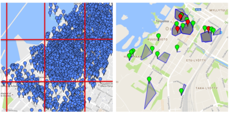
3.5.Rectangular grid – RG algorithm
The EUA approach has the disadvantage that it is possible that the resulting clusters include venues, which are, in reality, quite far apart (e.g. in urban areas where the density of venues is low). This can be realistically problematic, since it is unlikely that a venue that’s, for example, 700 m away from the reference point, can actually play some role in the reference point’s avgCM evolution. To limit this problem, the Rectangular Grid (RG) approach separates the urban area into smaller subsections (“tiles”), which are of a rectangular configuration and whose dimensions (height and width) are customisable (Fig. 1 left), attempting to split the area into tiles of the same size. For this approach, we first establish a “bounding box” using the maximum and minimum latitude and longitude values of all venues in an urban area. Then, a step-wise process separates the area into rectangular tiles with the dimensions set by the user. A side-effect of this algorithm is that tiles in the eastern and southern edges of an area can result in smaller than prescribed sizes, since the area is not always exactly divisible by the specified tile size. This process results in a set of tiles, which contain a varying density of venues. To assess a reference point’s avgCM evolution, we can therefore use the same steps in EUA approach, but only for the tile which contains the reference point. However, in the EUA approach, the k-means clustering step used a simple formula to determine an appropriate value for k, but this is not appropriate for the smaller tiles, given their variable venue density, which can mean too few, or too many venues in a given tile. Therefore, as a first step, we attempt to obtain a better estimate for k, with the following approach. For every tile, we iteratively run the DBSCAN algorithm on each tile’s venues, to identify clusters, starting with an ϵ value of 0.015 and setting the
3.6.Smart grid – SG algorithm
The Rectangular Grid approach has one major disadvantage: the way venues are separated is somewhat blind to the geography and spatial characteristics of the urban area. For example, tiles may contain a large amount of empty space (e.g. water), therefore resulting in separations which do not make spatial sense. To overcome this difficulty, we devised a third approach (Smart Grid – SG), which attempts to dynamically identify a subsection of the entire area to use, in order to predict the evolution of the avgCM of a specific reference point. To do this, we first run a k-means algorithm over the entire area. The k-value can be set by the user, and this results in what we term “smart tiles”. In each of the resulting clusters, we run an iterative version of the DBSCAN algorithm, starting with an ϵ value of 0.015 and progressively increasing it by 0.005 until there are no more than 25% unclustered venues in each of the k-means derived clusters. From the resulting paired number of cluster and tile venues values, we then derive a linear regression model which can be used to further run k-means to sub-cluster each original “smart-tile”, in order to extract a reference cluster to assess the estimated avgCM of the reference point (Fig. 1 right), which again is the average the resulting avgCM of each cluster.
4.Experimental evaluation
To determine the performance of our algorithms, we examined data collected for two similarly-sized cities, of approximately 200k inhabitants, one in Southeast Europe (Patras, Greece) and one in Northern Europe (Oulu, Finland), over two years (2014 and 2015). The dataset consists of
During these two years, several new businesses opened up in various locations, and since we were able to identify their first appearance on Foursquare and were able to track their evolution over the year, we are able to simulate the prediction of their social network evolution. A “new venue” in any given year is defined as a venue for which we first have a check-in record in that year, and that first record shows a total count of check-ins of 1. In total, we discovered 79 new venues (reference points) for Patras and 51 in Oulu for 2014, and 55 for Patras and 36 for Oulu in 2015. For each of these reference points thus, we picked a time window of 60 days after their first appearance in our dataset, and used this data to calculate the final true avgCM of the reference point, and as a dataset window to calculate the avgCM of the venues in the clusters which this reference point belonged to. As a metric of success, we considered that the avgCM of the reference point was “correctly predicted” if it fell within the 95% confidence interval for the avgCM of all the sub-clusters.
4.1.Empirical evaluation of algorithm parameters
The EUA algorithm relies on the DBSCAN ϵ parameter and
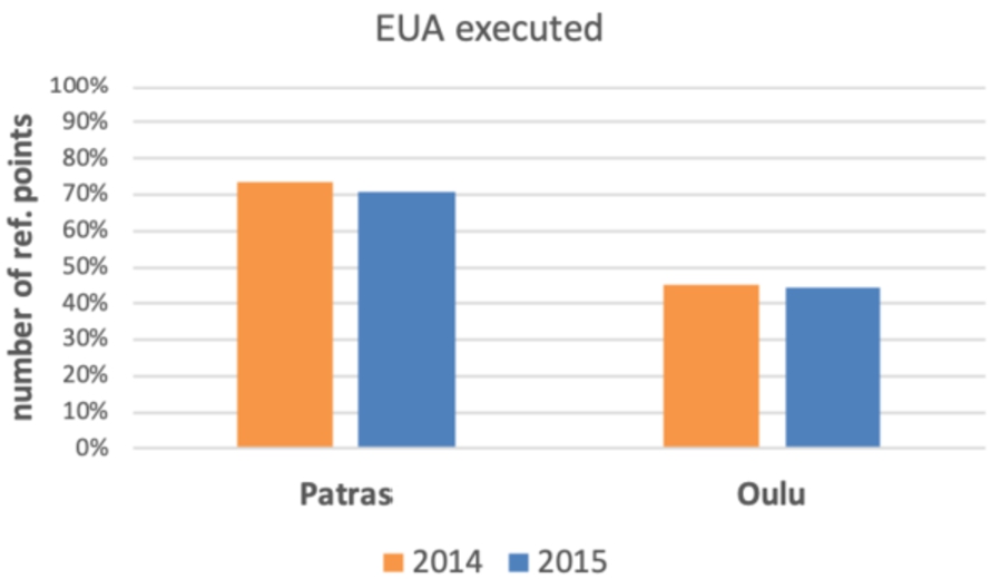
Fig. 2.
EUA execution success across all reference points.
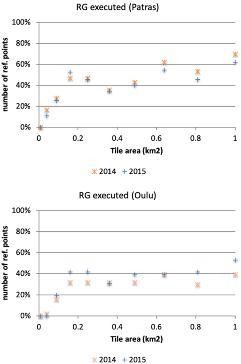
The RG and SG algorithms rely on two other user-defined parameters which are important for their operation. RG requires the specification of a tile size, and SG requires the initial k-value for its first clustering step. Depending on the values set for these parameters, the algorithms may not be able to execute for a particular reference point. For example, if the point is at a very sparsely populated area, it might not be possible for DBSCAN to derive any suitable clusters (remember that we specified that a cluster must have a minimum number of 3 venues). Therefore, as a first step, we aimed to determine parameter values which minimised the number of reference points for which the algorithms were “not executed” (NE). For RG’s tile size, we used a square configuration, setting the height of the tile equal to its width, and experimented with values starting at 100 m and incrementally going up to 1000 m, using a step of 100 m. From Fig. 3, we note that for the city of Patras, the number of NE reference points reaches minimal values for both years, with a tile size set to
Fig. 3.
RG execution success across all reference points.
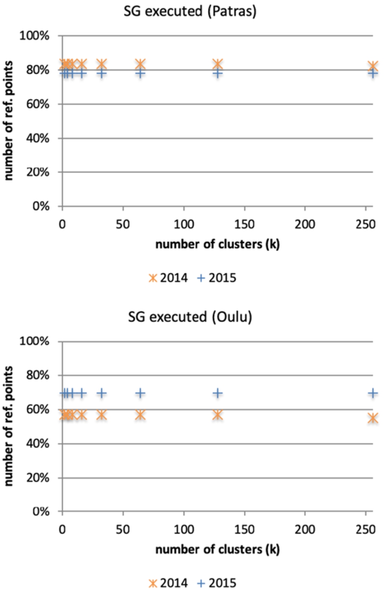
For SG, we experimented with values of k between 1 and 256, increasing by powers of two (i.e.
Fig. 4.
SG execution success across all reference points.
4.2.Algorithm performance
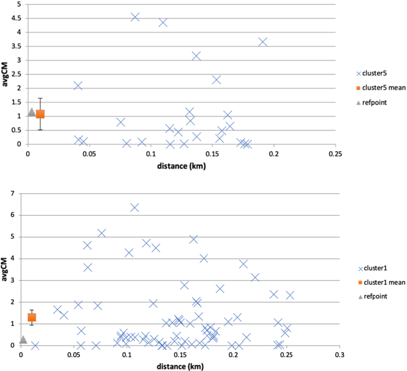
We examined the performance of the algorithms using the different value parameters to determine whether they also have an impact on the ability of the algorithms to correctly predict the social network evolution of the reference points in these two years. As explained previously, we define a prediction to be correct, if the observed avgCM metric of the reference point falls within range of the mean avgCM ± 95% c.i. of the other venues in its cluster. This is illustrated in Fig. 5, where examples of reference points falling inside and outside the cluster mean range are shown. This effectively transforms our problem into a classification problem, where classes are defined by a range of values that are the mean avgCM ± 95% c.i. in a cluster. Thus, for performance measuring purposes, we can use the recall metric defined as true positives over the sum of true positives and false negatives. In this case, true positives are those reference points whose avgCM metric falls within their cluster’s range, and false negatives are those points whose avgCM metric falls outside their cluster’s range (i.e. the algorithm was not able to properly assign a class to these reference points). We present results as a percentage of correctly predicted reference points over all reference points, and as an adjusted percentage over the number of reference points for which the algorithm was able to execute.
Fig. 5.
Examples of reference point actual evolution against cluster mean range. In the top example, the reference point’s avgCM falls within the cluster’s range (mean ± 95% c.i.), while in the bottom example it does not. Cluster point avgCM values are plotted against distance from the reference point. The cluster mean is plotted at a distance proximal to the reference point (i.e. not the cluster spatial centroid) to assist visualisation.
We estimated the performance of EUA for both cities in both years. As per Fig. 6, the algorithm is able to correctly predict the social evolution in a relatively small fraction of the reference points (2014 Patras: 29.1%, Oulu 21.6%; 2015 Patras: 29.1%, Oulu: 16.7%). Considering the adjusted performance values (i.e. discounting the number of points for which the algorithm did not execute), the situation improves somewhat, but the performance is still quite low (2014 Patras: 39.7%, Oulu 47.8%; 2015 Patras: 41.0%, Oulu: 37.5%).
Next, we estimate the performance of RG for the various tile sizes (Fig. 7). For Patras, we observe an increase trend in the percentage number of correctly predicted reference points, reaching a maximum of 31.6% in 2014 and 30.9% 2015, with a tile size of
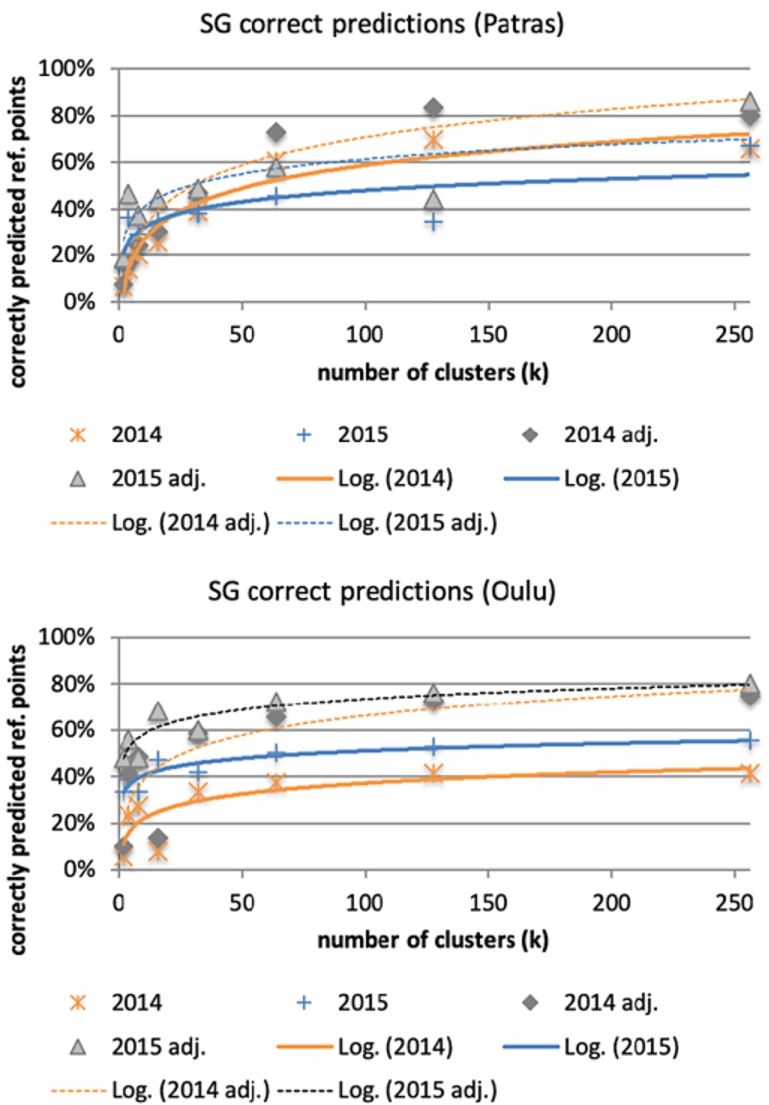
Finally, we estimate the performance of SG for the various cluster sizes (Fig. 8). For Patras, we observe a logarithmic increase in the correct predictions with the number of clusters, for both recall metrics (over all points, and adjusted). The correlation between the number of clusters and correctly predicted reference points is statistically significant in both years (Spearman’s two tailed 2014
Fig. 6.
EUA performance across all reference points and across executed reference points only (adj.).
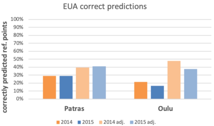
Fig. 7.
RG execution success across all reference points.
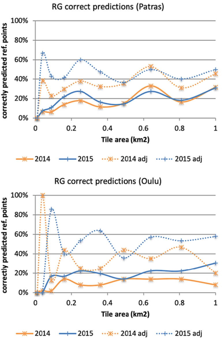
Fig. 8.
SG execution success across all reference points.
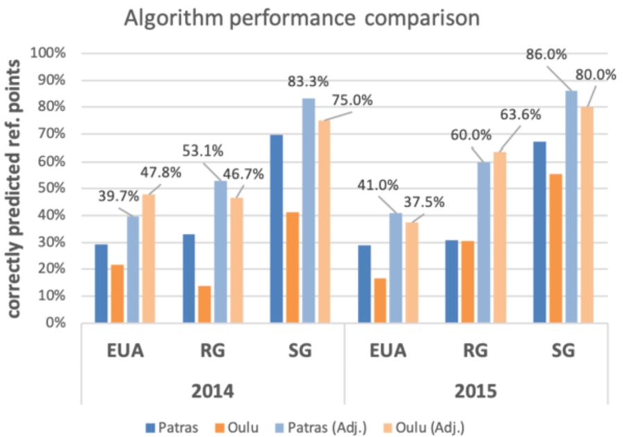
We present in Fig. 9 each algorithm’s best performance, with the criterion that the algorithm will have executed for at least 10 reference points. The SG algorithm outperforms the baseline EUA and the RG algorithm consistently, achieving better prediction performance in both cities and for both years. This performance advantage holds when all reference points are considered, and is substantially increased when calculated over only those reference points for which the algorithm was able to execute. One significant advantage of SG also seems to be the fact that its ability to execute is invariant to the running parameters, therefore leaving out a constantly small number of reference points for which it is unable to provide a prediction.
Fig. 9.
Algorithm performance under optimal parameters.
5.Influence of venues in SG clusters for prediction accuracy
With the previous results in mind and given that SG seems to perform better than other approaches in clustering venues, we further investigated alternative approaches to predicting the evolution of the check-ins for reference points. We concentrate this further investigation on the city of Patras and the year 2015, based on the previous results.
A detailed look into our dataset revealed that cluster (non-reference) points can exhibit a range of behaviours in the timeframe used for prediction (e.g. see the individual avgCM metric of cluster points in Fig. 5). This became even more apparent when we divided each reference points’ two-month period into 9 week bins (the last week bin has fewer days) and observed that check-in patterns in the respective clusters followed three distinct patterns. Some cluster points’ evolution remains static (i.e. they receive no check-ins), others exhibit a somewhat linear increase in their check-ins, and finally a third category of venues receive a varying number of check-ins, throughout the two month periods used in our dataset for prediction. In this sense, the weekly check-in patterns of some cluster points carry more information than others. Zero and linear increase venues make predictions ostensibly easy. On the other hand, venues with highly variable patterns (i.e. large deviations in the intra-week check-in volume) might make these predictions more unstable.
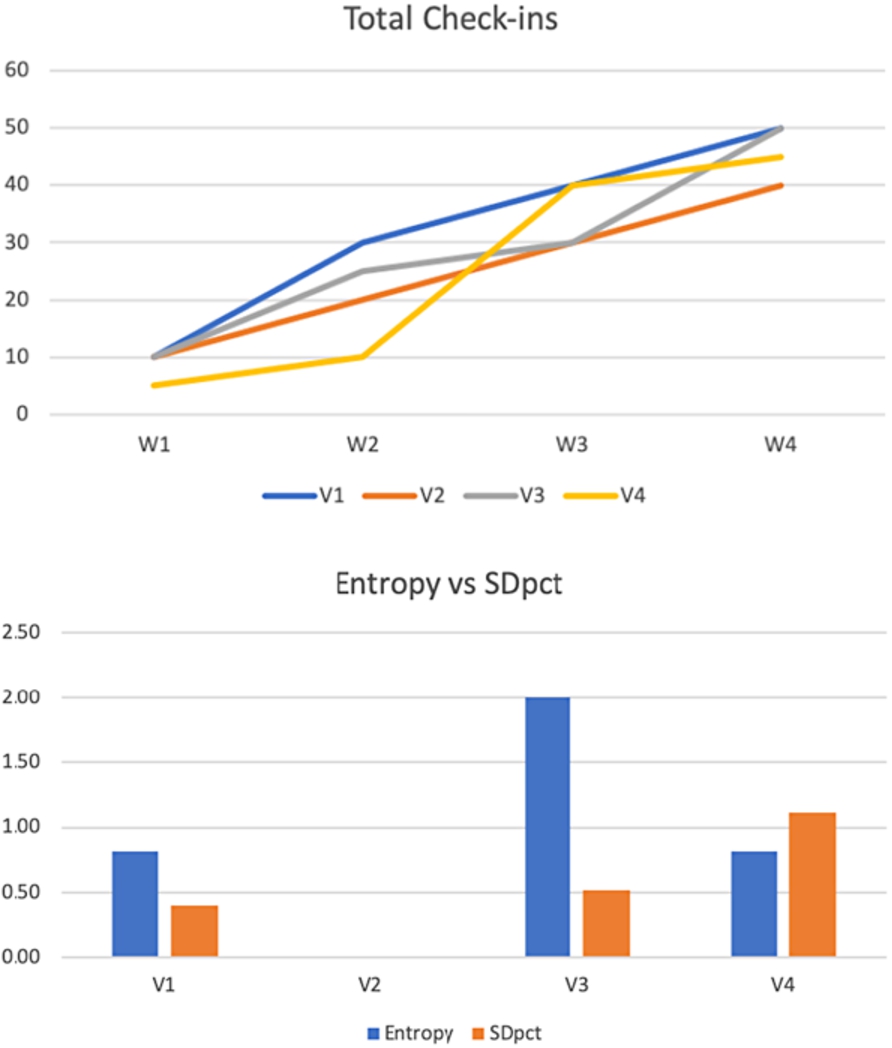
To illustrate this point, consider an example as follows. Supposing a fictional reference point
Table 1
Weekly check-in patterns and metrics for venues in a hypothetical cluster
| Venue | Total check-ins | Entropy | σ | SDpct | |||||
| 50 | 10 | 20 | 10 | 10 | 12.5 | 0.811 | 5.000 | 0.400 | |
| 40 | 10 | 10 | 10 | 10 | 10 | 0.000 | 0.000 | 0.000 | |
| 50 | 10 | 15 | 5 | 20 | 12.5 | 2.000 | 6.455 | 0.516 | |
| 45 | 5 | 5 | 30 | 5 | 11.25 | 0.811 | 12.500 | 1.111 |
As can be seen in Fig. 10 (top), venue
Fig. 10.
Weekly check-in evolution for the hypothetical cluster (top) and resulting metric comparison (bottom).
In the previous experiments, we considered data from all venues in a reference point’s cluster, but it could be possible that a selective approach might have positive effects on the prediction accuracy. Since our time window T was 60 days, which spreads over 9 weeks, for each cluster point, we constructed a feature vector consisting of the total new check-ins for
As a metric for performance, we adopt a slightly different approach to the previous analysis and use the root mean square error (
5.1.Using all venues as candidates for prediction
First, we start by reporting the results by considering the effect of cluster venue entropy and SDpct on
Fig. 11.
Filtering cluster venues by entropy threshold.
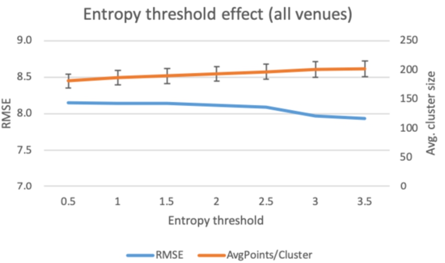
Fig. 12.
Filtering cluster venues by SDpct threshold.
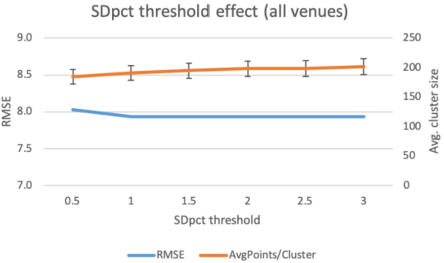
Regarding SDpct, we follow the same approach as with the entropy threshold. The maximum value is 2.828 (
5.2.Using venues with at least one check-in as candidates for prediction
Next, we limit the clusters to include only venues which display at least one check-in during the 2-month period. We repeat the previous analysis using an entropy and an SDpct-based filter. Starting off with the entropy filter, the first observation is that the limitation to venues that exhibit at least one check-in, results in a dramatic reduction in the number of venues considered in the clusters (
Fig. 13.
Filtering cluster venues with
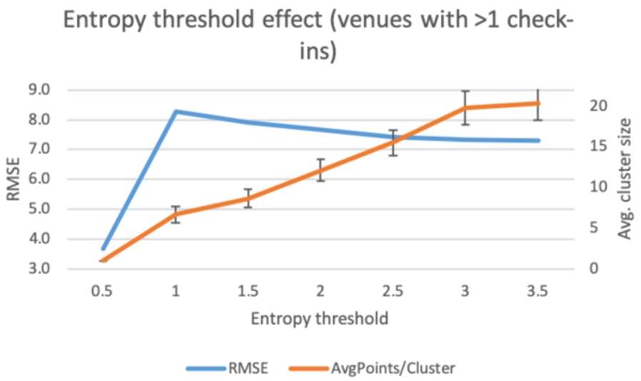
Fig. 14.
Filtering cluster venues with
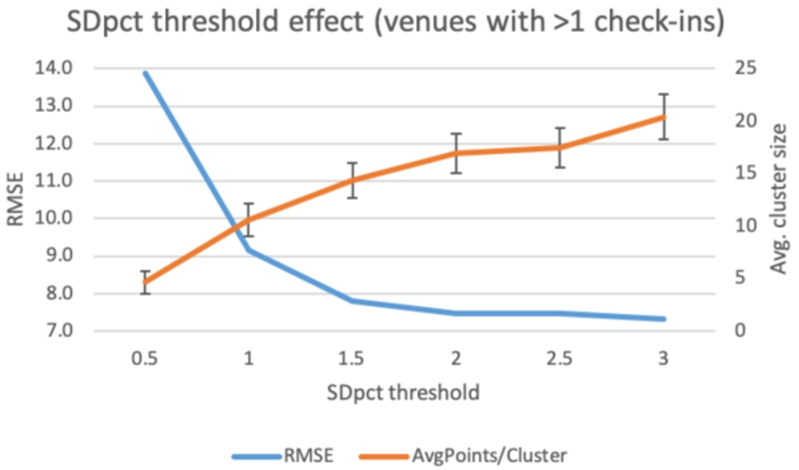
Continuing the analysis using the SDpct threshold, we note that the issue of using a low threshold value (0.5) that results in too few clusters with available venues (as in the entropy filter), does not arise. This is expected, since SDpct is more likely to take arbitrary values, compared to entropy where, as demonstrated in our hypothetical example, it is far more likely that multiple venues may end up having the same entropy value. Again, in this analysis, we note the large reduction in average cluster size (
5.3.Summary of findings
Paired together, all the preceding analyses results demonstrate that the consideration of venues that exhibit little variability in their check-in patterns, is unnecessary for the prediction of the evolution of new venues, and that the inclusion of venues with highly variable check-in patterns is beneficial for the reduction of prediction error, regardless of the type of metric used to capture this variation.
Table 2
SG algorithm performance using the
| Venue filter | All cluster venues | Cluster venues with |
| SDpct | 14.63% | 41.46% |
| Entropy | 14.63% | 41.46% |
To illustrate this, we perform an analysis as per Section 4.2, to assess the classification of reference points according to the
In our initial analysis, we didn’t exclude points with little variation, adopting an agnostic approach to the selection of data. By this approach, it could be assumed that cases where little variation is exhibited (e.g. linear increase) should bias predictions for a new venue accordingly (i.e. also increasing linearly). However, in hindsight, perhaps an explanation for the improved performance is that it’s not “natural” for a place to exhibit a steady stream of check-ins (e.g. these could originate from staff, or regular customers). On the other hand, a more variable pattern might be closer to the check-in patterns a new venue can expect, therefore explaining the benefit in predictions.
6.Discussion and conclusions
We presented three algorithms to solve the problem of predicting the evolution of check-ins for a venue in a social network, based on the check-in behaviour of users in the venues in its neighbourhood. Since the number of check-ins can be associated with the visitation patterns in physical stores, and by extension, their commercial success, we have demonstrated an ability to predict the commercial success of a new physical business, in the context of a smart city. Our approach has the benefit that it is based on readily available data and can be deployed for any urban environment with a considerable venue density. We have demonstrated that the SG algorithm is able to dynamically adapt to the local spatial characteristics of urban environments, better than the EUA and RG approaches. It successfully identifies appropriate neighbours for a target venue, thus being able to predict its evolution on social networks based on these neighbours. Even more, we have demonstrated that not all neighbours matter for prediction. Those neighbours that do not exhibit any new check-ins in the reference period actually detriment the algorithm’s performance and add unnecessary computational demands on the system. The results of the SG algorithm on two similar-sized cities in countries with societal differences (north and southern Europe) show that the approach is possibly generalisable globally.
Contrary to other approaches in current literature [5,12,13,19], we did not limit ourselves to a specific type of business (e.g. food), but allowed the algorithm to execute for all types of businesses in the input dataset. Further improvements could include limiting the input dataset to just those neighbouring businesses which are of the same type as the target. We could also have chosen to consider only business types which can be considered as complementary, e.g., if the target is a restaurant, we could include restaurants, cafes and bars, since they also typically serve food, or only those businesses which are open at the same time as the target business. However, such approaches would require a more intimate knowledge of how the retail market operates in a given urban environment (e.g., mobility and temporal aspects of visitation in venue types), which is difficult to acquire. In further work, we would like to explore the performance of our algorithm in different scale urban environments (e.g. large dense urban areas like Manhattan, NY). Further work is also required in defining more appropriate classification targets, since in this case we employed a rather simple metric, and to examine different types of engagement in social network presence, such as number of likes, ratings, customer comments and feedback.
Acknowledgements
We would like to thank the reviewers of our original paper [18] and especially the reviewers of this extended version, for their significant contributions towards improving the final article. Research in this paper was funded by the Hellenic Government NSRF 2014-2020 (Filoxeno 2.0 project, T1EDK-00966).
References
[1] | S. Bandini, M.L. Federici and S. Manzoni, A qualitative evaluation of technologies and techniques for data collection on pedestrians and crowded situations, in: Proceedings of the 2007 Summer Computer Simulation Conference, SCSC ’07, Society for Computer Simulation International, San Diego, CA, USA, (2007) , pp. 1057–1064. ISBN 978-1-56555-316-3. |
[2] | Forrester data: Digital-influenced retail sales forecast, 2017 to 2022 (US). https://www.forrester.com/report/Forrester+Data+DigitalInfluenced+Retail+Sales+Forecast+2017+To+2022+US/-/E-RES140811. |
[3] | W. Friske and S. Choi, Another look at retail gravitation theory: History, analysis, and future considerations, Academy of Business Disciplines Journal 5: (1) ((2013) ), 88–106. |
[4] | Y. Fukuzaki, M. Mochizuki, K. Murao and N. Nishio, A pedestrian flow analysis system using wi-fi packet sensors to a real environment, in: Proceedings of the 2014 ACM International Joint Conference on Pervasive and Ubiquitous Computing: Adjunct Publication, UbiComp ’14 Adjunct, ACM, New York, NY, USA, (2014) , pp. 721–730. ISBN 978-1-4503-3047-3. doi:10.1145/2638728.2641312. |
[5] | P.I. Georgiev, A. Noulas and C. Mascolo, Where businesses thrive: Predicting the impact of the Olympic games on local retailers through location-based services data, in: Eighth International AAAI Conference on Weblogs and Social Media, (2014) . |
[6] | O. González-Benito, Spatial competitive interaction of retail store formats: Modeling proposal and empirical results, Journal of Business Research 58: (4) ((2005) ), 457–466. doi:10.1016/j.jbusres.2003.09.001. |
[7] | D. Karamshuk, A. Noulas, S. Scellato, V. Nicosia and C. Mascolo, Geo-spotting: Mining online location-based services for optimal retail store placement, in: Proceedings of the 19th ACM SIGKDD International Conference on Knowledge Discovery and Data Mining, KDD ’13, ACM, New York, NY, USA, (2013) , pp. 793–801. ISBN 978-1-4503-2174-7. doi:10.1145/2487575.2487616. |
[8] | M.B. Kjærgaard, M. Wirz, D. Roggen and G. Tröster, Mobile sensing of pedestrian flocks in indoor environments using WiFi signals, in: 2012 IEEE International Conference on Pervasive Computing and Communications, (2012) , pp. 95–102. doi:10.1109/PerCom.2012.6199854. |
[9] | M.B. Kjærgaard, M. Wirz, D. Roggen and G. Tröster, Detecting pedestrian flocks by fusion of multi-modal sensors in mobile phones, in: Proceedings of the 2012 ACM Conference on Ubiquitous Computing, UbiComp ’12, ACM, New York, NY, USA, (2012) , pp. 240–249. ISBN 978-1-4503-1224-0. doi:10.1145/2370216.2370256. |
[10] | A. Komninos, V. Stefanis, A. Plessas and J. Besharat, Capturing urban dynamics with scarce check-in data, IEEE Pervasive Computing 12: (4) ((2013) ), 20–28. doi:10.1109/MPRV.2013.42. |
[11] | M. Li, Y. Sun and H. Fan, Contextualized relevance evaluation of geographic information for mobile users in location-based social networks, ISPRS International Journal of Geo-Information 4: (2) ((2015) ), 799–814. doi:10.3390/ijgi4020799. |
[12] | J. Lin, R. Oentaryo, E.-P. Lim, C. Vu, A. Vu and A. Kwee, Where is the goldmine?: Finding promising business locations through Facebook data analytics, in: Proceedings of the 27th ACM Conference on Hypertext and Social Media, HT ’16, ACM, New York, NY, USA, (2016) , pp. 93–102. ISBN 978-1-4503-4247-6. doi:10.1145/2914586.2914588. |
[13] | J. Lin, R.J. Oentaryo, E.-P. Lim, C. Vu, A. Vu, A.T. Kwee and P.K. Prasetyo, A business zone recommender system based on Facebook and urban planning data, in: Advances in Information Retrieval, N. Ferro, F. Crestani, M.-F. Moens, J. Mothe, F. Silvestri, G.M. Di Nunzio, C. Hauff and G. Silvello, eds, Lecture Notes in Computer Science, Springer International Publishing, (2016) , pp. 641–647. ISBN 978-3-319-30671-1. doi:10.1007/978-3-319-30671-1_47. |
[14] | T. Nam and T.A. Pardo, Conceptualizing smart city with dimensions of technology, people, and institutions, in: Proceedings of the 12th Annual International Digital Government Research Conference: Digital Government Innovation in Challenging Times, Dg.o ’11, ACM, New York, NY, USA, (2011) , pp. 282–291. ISBN 978-1-4503-0762-8. doi:10.1145/2037556.2037602. |
[15] | A. Noulas, S. Scellato, R. Lambiotte, M. Pontil and C. Mascolo, A tale of many cities: Universal patterns in human urban mobility, PLoS ONE 7: (5) ((2012) ), e37027. doi:10.1371/journal.pone.0037027. |
[16] | E. Panizio, Accessibility of touristic venues in Amsterdam: A methodology to collect, assess and validate the attractiveness and accessibility of touristic venues from data extracted using Twitter as urban sensor: A.M.S. case, 2015. |
[17] | A. Pansari and V. Kumar, Customer engagement: The construct, antecedents, and consequences, Journal of the Academy of Marketing Science 45: (3) ((2017) ), 294–311. doi:10.1007/s11747-016-0485-6. |
[18] | G. Papadimitriou, A. Komninos and J. Garofalakis, Supporting Retail Business in Smart Cities Using Urban Social Data Mining, IEEE, (2019) . |
[19] | A.M.B.M. Rohani and F.-F. Chua, Location analytics for optimal business retail site selection, in: Computational Science and Its Applications – ICCSA 2018, O. Gervasi, B. Murgante, S. Misra, E. Stankova, C.M. Torre, A.M.A.C. Rocha, D. Taniar, B.O. Apduhan, E. Tarantino and Y. Ryu, eds, Lecture Notes in Computer Science, Springer International Publishing, (2018) , pp. 392–405. ISBN 978-3-319-95162-1. doi:10.1007/978-3-319-95162-1_27. |
[20] | S. Salat, M. Chen and F. Liu, Planning energy efficient and livable cities, Technical Report, 93678, World Bank, 2014. |
[21] | T.H. Silva, P.O.S.V. de Melo, J.M. Almeida and A.A.F. Loureiro, Social media as a source of sensing to study city dynamics and urban social behavior: Approaches, models, and opportunities, in: Ubiquitous Social Media Analysis, M. Atzmueller, A. Chin, D. Helic and A. Hotho, eds, Lecture Notes in Computer Science, Springer, Berlin, Heidelberg, (2013) , pp. 63–87. ISBN 978-3-642-45392-2. doi:10.1007/978-3-642-45392-2_4. |
[22] | F. Terroso-Saenz and A. Muñoz, Land use discovery based on volunteer geographic information classification, Expert Systems with Applications 140: ((2020) ), 112892. doi:10.1016/j.eswa.2019.112892. |
[23] | A. Venerandi, G. Quattrone, L. Capra, D. Quercia and D. Saez-Trumper, Measuring urban deprivation from user generated content, in: Proceedings of the 18th ACM Conference on Computer Supported Cooperative Work & Social Computing, CSCW ’15, ACM, New York, NY, USA, (2015) , pp. 254–264. ISBN 978-1-4503-2922-4. doi:10.1145/2675133.2675233. |
[24] | J. Weppner and P. Lukowicz, Bluetooth based collaborative crowd density estimation with mobile phones, in: 2013 IEEE International Conference on Pervasive Computing and Communications (PerCom), (2013) , pp. 193–200. doi:10.1109/PerCom.2013.6526732. |
[25] | B. Zhan, D.N. Monekosso, P. Remagnino, S.A. Velastin and L.-Q. Xu, Crowd analysis: A survey, Machine Vision and Applications 19: (5) ((2008) ), 345–357. doi:10.1007/s00138-008-0132-4. |


