
Machine Learning Selection of Most Predictive Brain Proteins Suggests Role of Sugar Metabolism in Alzheimer’s Disease
Abstract
Background:
The complex and not yet fully understood etiology of Alzheimer’s disease (AD) shows important proteopathic signs which are unlikely to be linked to a single protein. However, protein subsets from deep proteomic datasets can be useful in stratifying patient risk, identifying stage dependent disease markers, and suggesting possible disease mechanisms.
Objective:
The objective was to identify protein subsets that best classify subjects into control, asymptomatic Alzheimer’s disease (AsymAD), and AD.
Methods:
Data comprised 6 cohorts; 620 subjects; 3,334 proteins. Brain tissue-derived predictive protein subsets for classifying AD, AsymAD, or control were identified and validated with label-free quantification and machine learning.
Results:
A 29-protein subset accurately classified AD (AUC = 0.94). However, an 88-protein subset best predicted AsymAD (AUC = 0.92) or Control (AUC = 0.92) from AD (AUC = 0.98). AD versus Control: APP, DHX15, NRXN1, PBXIP1, RABEP1, STOM, and VGF. AD versus AsymAD: ALDH1A1, BDH2, C4A, FABP7, GABBR2, GNAI3, PBXIP1, and PRKAR1B. AsymAD versus Control: APP, C4A, DMXL1, EXOC2, PITPNB, RABEP1, and VGF. Additional predictors: DNAJA3, PTBP2, SLC30A9, VAT1L, CROCC, PNP, SNCB, ENPP6, HAPLN2, PSMD4, and CMAS.
Conclusion:
Biomarkers were dynamically separable across disease stages. Predictive proteins were significantly enriched to sugar metabolism.
INTRODUCTION
Early elucidation of Alzheimer’s disease (AD) is pivotal for constructing clinically impactful treatments. However, the pathophysiology of AD and the driving biochemical changes are not fully understood. Assessment of changes in protein expressions in the brain may assist in elucidation of multi-factorial biochemical changes that lead to AD [1]. Given the complexity and heterogeneity of AD, no single protein is likely to be predictive of all mechanisms or phenotypes which result in AD [2]. Nonetheless, predictive protein models may suggest novel disease mechanisms, improve assessment of patient risk, and signify disease stage-dependentbiomarkers [3].
This work identifies protein subsets that differentiate diagnostic labels for AD. AD diagnosis is often based on clinically measured functional cognitive decline. AD diagnosis is typically determined using a battery of neuropsychological tests in combination with suggestive imaging, genomic, or other clinical features. Common cognitive tests used in AD diagnosis include the Montreal Cognitive Assessment or Consortium to Establish a Registry for Alzheimer’s Disease (CERAD) neuropsychological battery [4]. There is no universal definition of asymptomatic AD (AsymAD). AsymAD is typically characterized by changes in age-adjusted biomarkers, such as increase in amyloid-β and tau in the brain, without overt presence of cognitive decline [5]. Control subjects typically show no overt cognitive losses and no significant change in age-adjusted biomarkers.
In particular, identification of subsets of proteins that better predict and stratify the asymptomatic AD stage is pivotal. Earlier identification of patients likely to transition to AD could enable earlier intervention. The ability to intervene early is likely key to improving outcomes, such as slowing progression or improving symptom-related quality of life. The amyloid-β cascade, tauopathy, and Apolipoprotein E (ApoE) are known aberrant protein signatures in AD [6–9]. However, other proteins may provide earlier clues during asymptomatic changes. For example, metabolomic [10], lipidomic, and inflammation-related proteins have also been suggested to be involved in aging and dementia [11].
The study goal was to determine which proteins in the brain (beyond amyloid-β and phosphorylated tau) are most important for classifying a human subject as either control, AsymAD, or AD. Data consisted of 3,334 brain tissue-derived proteins measured via label-free quantification (LFQ) [3] in six different clinical cohorts. Machine learning classification with recursive feature elimination was used to select the “best” or most predictive proteins.
METHODS
Methods consist of data collection and preprocessing; protein selection using a machine learning algorithm to identify the “best” subset of proteins to predict patient diagnostic classification; validation of the algorithm to accurately classify control, AsymAD, or AD patients using only the identified “best” subset of predictive proteins; and assessment of predictive protein functions. All data preprocessing, machine learning, and analysis was performed in Python 3.6.
Patient diagnostic class labels
Note that the patient diagnostic labels (Control, AsymAD, AD) were inherited from previously published work. Briefly, according to the definitions outlined by Johnson et al. [3], the neuropathological diagnostic classes were determined using CERAD criteria to quantify neuritic plaque distribution and Braak staging to quantify extent of neurofibrillary tangle pathology.
Data used for protein biomarker identification
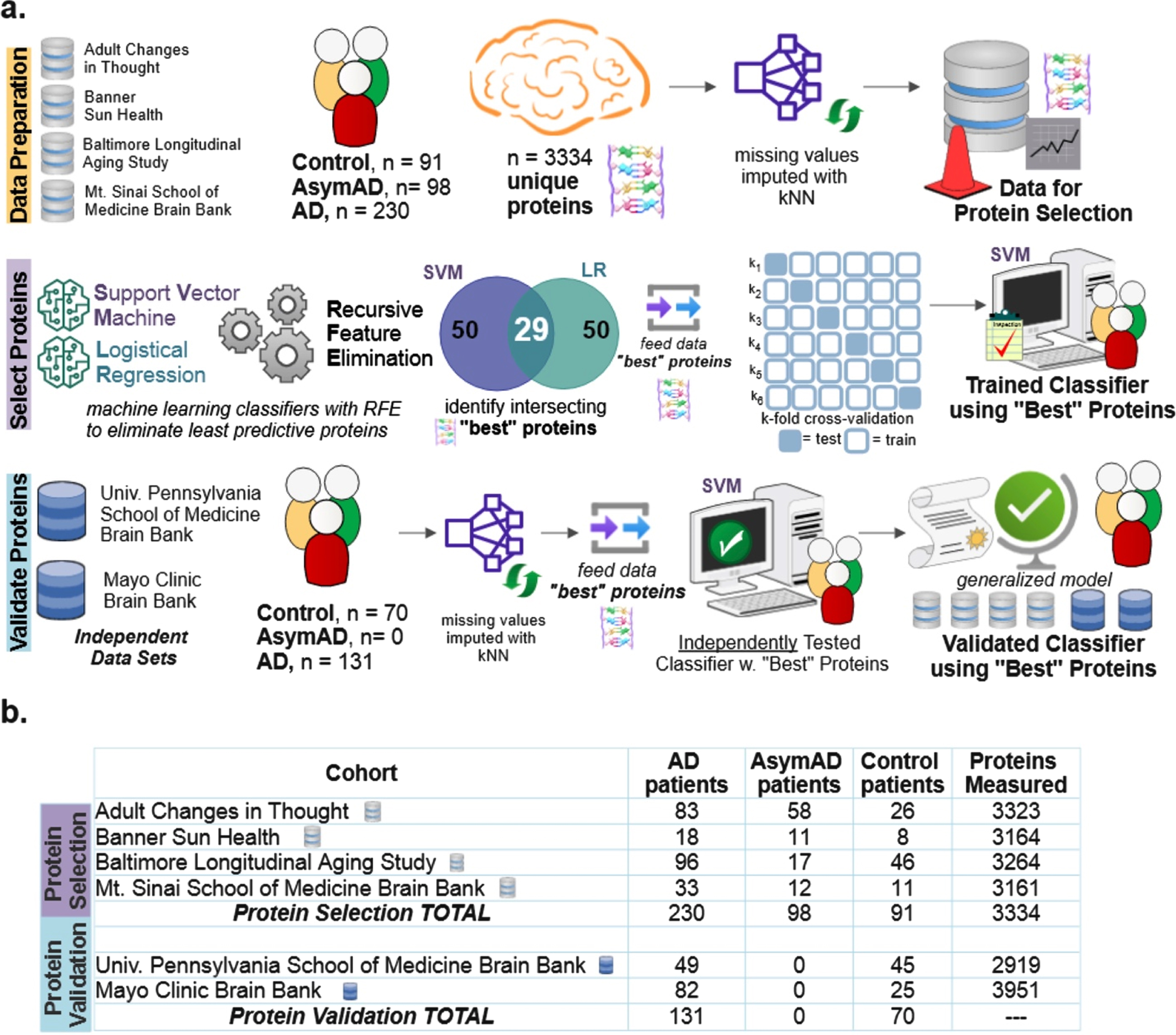
Six public data sets were utilized [3]: Baltimore Longitudinal Study of Aging (BLSA) [12], Banner Sun Health Research Institute (Banner) [13], Mount Sinai School of Medicine Brain Bank (MSSB) [2], Adult Changes in Thought Study (ACT), Mayo Clinic Brain Bank and University of Pennsylvania School of Medicine Brain Bank. Four data sets (n = 419 subjects) were utilized for initial model construction and “best” protein selection: BLSA, Banner, ACT, and MSSB. Two data sets (n = 201 subjects) were used to independently validate the ability of the selected best protein subset to classify the diagnostic label of subjects: Mayo and UPenn cohorts. For all cohorts except Mayo, the tissue was taken from the dorsolateral prefrontal cortex. For the Mayo cohort, the tissue was taken from the temporal cortex. As shown in Fig. 1a as part of data preparation, missing values were imputed using the k-nearest neighbor (kNN). The optimal number of neighbors for imputation of missing values was determined to be 20 (Supplementary Figure 1). Figure 1b shows the number of subjects and quantified proteins for each cohort. Supplementary Figure 2 illustrates the overall distribution of amyloid-β, tau, APP, CERAD score, and Braak in the data sets used for protein selection. Because amyloid-β and tau were utilized to determine the class labels [3] in the original data sets, tau and amyloid-β levels are not explicitly utilized as part of the protein identification and selection process here. Inclusion of amyloid-β and tau would have resulted in a circular analysis that confounded results. However, their pathways are indirectly represented via upstream biomarkers like APP.
Fig. 1
Diagram explaining the data and machine learning pipeline to identify a subset of “best” predictive protein biomarkers to accurately classify Alzheimer’s disease (AD), asymptomatic Alzheimer’s disease (AsymAD), or Control. a) Machine learning pipeline consisted of data preparation, protein selection, and model validation with selected proteins. Data was prepared by aggregating four cohorts (n = 419 subjects, n = 3,334 unique proteins) and imputing missing values using k-nearest neighbor algorithm. The most predictive proteins were selected using recursive feature elimination (RFE) to construct and train a support vector machine (SVM) classifier that can predict diagnosis using only the selected “best” proteins (n = 29 or n = 88 best predictive proteins). Finally, the developed classifier model was independently validated using 2 additional cohorts (n = 201 subjects) to ensure the model’s performance generalizes to new data. b) Details of six data cohorts used in protein selection (4 cohorts) and validation (2 cohorts), including sample sizes.
Protein selection using machine learning
As shown in the protein selection row of Fig. 1a, proteins from the selection cohort (data from BLSA, Banner, ACT, and MSSB) were selected using a combination of classification algorithms with recursive feature elimination (RFE). RFE is a feature selection algorithm which recursively eliminates less important data features until a pre-defined number of features remain in the dataset. In this study, the “features” are the measured proteins. This iterative procedure is an instance of backward selection [14]. RFE [14] is used to determine the most predictive proteins for successful classification. The resultant predictive protein subset was then used to classify each subject as either control, AsymAD, or AD.
RFE is a wrapper-based feature selection algorithm where recursive rounds of elimination are used to determine the subset of proteins that best predict patient diagnostic classification. The final set of selected predictive proteins is, in part, sensitive to the classification method. Thus, two popular linear classification methods were independently used with RFE in the scikit-learn package of Python: support vector machine (SVM) and logistic regression (LR), both with linear kernels [15]. The two classifiers, SVM and LR, separately select a specified number of most predictive proteins equal to the RFE criterion. The RFE criterion is the number of proteins the algorithm is allowed to retain. Note that other classifiers were also tried in place or in combination with SVM and LR. However, the intersection of proteins selected by SVM and LR was most consistent and accurate; hence, all results shown utilized this method.
Proteins are selected based on their superior classification ability as quantitatively measured by the area under the precision-recall curve (AUPRC). The intersecting most predictive proteins become the “best proteins”. The RFE algorithm assessed RFE criterions ranging from 10 to 150 proteins. For example, the Venn diagram of Fig. 1a for protein selection illustrates that an RFE criterion of 50 for SVM and LR resulted in an intersecting set of 29 best proteins. Upon completion of protein selection using RFE, a new SVM classifier is constructed, trained, and validated to classify diagnosis (AD, control, AsymAD) using only the selected best proteins. With three classes (control, AsymAD, AD), a one versus rest approach was utilized (AD versus NonAD, AsymAD versus non-AsymAD, control versus non-control).
Note that alternative methods to RFE to identify the most predictive proteins were considered and tried on LFQ as well as held out data: penalized lasso (Supplementary Figure 5), random forest feature importance (Supplementary Figure 6), and statistical differential protein expression using the f-statistic (Supplementary Figure 7). Also, random forests were coupled with RFE to have a more stringent selection criterion - including a protein only when it is selected by three algorithms: SVM, logistic regression, and random forests (Supplementary Figure 8). Performance comparison to neural network, which played no role in feature selection, is also shown in Supplementary Figures 5–8. In some cases, the alternate methods shown in the supplementary figures performed marginally better on the UPenn dataset, which has only binary labels (Control/AD). In all cases, RFE chosen proteins performed substantially better on the LFQ dataset which has more samples (n = 419), classes (Control/AsymAD/AD), and comprised 4 different datasets (ACT, MSSB, Banner, BLSA) (Fig. 1). Because of its superior multi-class performance and generalizability, the RFE-based primary method shown in Fig. 1a was used to produce all results shown in the mainarticle.
Validation of “best” protein subsets to classify diagnosis
As shown in the Protein Validation row of Fig. 1a, the trained SVM classifier was independently tested using validation cohort data (Mayo, UPenn data sets). As part of independent validation, the best set(s) of proteins determined during protein selection with RFE was used to predict validation cohort diagnostic classes. However, there were a couple of exceptions due to required data harmonization. In the Mayo cohort, one of the “best” proteins was not quantified (CROCC|Q5TZA2) and a different protein isoform was quantified for APP; APP|A0A0A0MRG2 was included for Mayo, instead of APP|E9PG40). Similarly, for the UPenn cohort, two of the “best” proteins were not quantified (C4A|P0C0L4, DMXL1|Q9Y485), and a different isoform was quantified for APP (APP|A0A0A0MRG2 instead of APP|E9PG40).
Confusion matrices illustrate true positives (TP), false positives (FP), true negatives (TN), and false negatives (FN) used to calculate classification performance. Additionally, a precision-recall curve (PRC) is generated to assess aggregate final model performance. PRC assesses the model’s classification accuracy when using only the “best” protein subsets to classify diagnosis. PRC is a plot of precision versus recall. Recall is defined as [TP/ (TP+FN)], and precision is defined as [TP/(TP+FP)]. Area under the curve (AUC) provides an aggregate measure of performance across all classification thresholds.
A separate unsupervised learning technique, t-stochastic neighbor embedding (t-SNE), was used to assess separability of AD, AsymAD, and Control subjects using only the selected best proteins subsets determined during supervised learning with RFE.
Finally, principal component analysis (PCA), a dimensional reduction technique, was used to explore and validate RFE criteria. The scree plot and elbow method were used to separately verify how many proteins are necessary to explain the preponderance of variance. The elbow approximated the number of intersecting proteins selected during RFE for optimal diagnostic classification.
Analysis of protein function modules
Selected proteins were matched to their protein function using the color modules and algorithms published by Johnson et al. [3]. There are 14 possible functional modules comprising the entire protein data set (n = 3,334 unique proteins). The percent composition of specific functional modules in the selected “best” protein subsets were compared to the original, full protein set. Significant differences were assessed using two-sided binomial tests at an alphaof 0.05.
RESULTS
A machine learning classification and recursive feature elimination process (Fig. 1a) determined which of 3,334 possible clinically measured proteins were most important for classifying control, AsymAD, or AD. RFE was used to identify the proteins that best predicted diagnostic class. Six public data sets were utilized (Fig. 1b). Four data sets (n = 419 subjects) were for protein selection, which consisted of identifying the “best proteins”. Two data sets (n = 201 subjects) were used for independent protein validation. Independent validation on unseen data ensured the model was generalizable. Hence, the model can correctly classify the diagnosis of new subjects using only the selected best protein subset(s). An RFE criterion of 50, which resulted in 29 best proteins, was found sufficient to distinguish AD from control. However, an RFE criterion of 150, which resulted in 88 best proteins, was found necessary to optimally distinguish AsymAD from AD.
Classification performance with 29 best proteins
Amyloid precursor protein (APP) is linked to the well-known amyloid-β pathway [16]. It was also selected by RFE as one of the 29 best proteins. Hence, it was important to carefully assess if APP was impacting or biasing classification compared to other proteins. Figure 2 illustrates the classification performance using APP alone (Fig. 2a-c), the selected 29 best proteins (Fig. 2d-f), and APP excluded from the panel of 29 proteins (Fig. 2g-i) for three datasets (LFQ, Mayo, and UPenn). Figure 2d illustrates the performance confusion matrix for the LFQ cohort, Fig. 2e the Mayo validation cohort, and Fig. 2f the UPenn validation cohort, with the selected 29 best proteins. For the LFQ cohort, the model correctly classified 186 of the 230 AD patients (80.87%), while 19 AD patients (8.2%) were misclassified as AsymAD, and 15 AD patients (6.5%) were misclassified as Control. For the Mayo validation cohort, where proteins were measured in the temporal cortex, 71 AD patients (86.6%) were correctly classified, whereas 11 AD patients were misclassified as Control. For the UPenn validation cohort, where proteins were measured in the dorsolateral prefrontal cortex, 37 AD patients were correctly classified, whereas 12 AD patients (24.5%) were misclassified as Control. Similar trend was seen in Fig. 2g-i when APP was removed from the panel of 29 best proteins and the remaining proteins were used. In summary, the exclusion of APP did not significantly diminish the ability of the remaining 28 proteins to predict diagnosis. This result indicates classification is not dependent on APP alone.
Fig. 2
Examination of classification performance for Alzheimer’s disease (AD), asymptomatic Alzheimer’s Disease (AsymAD), and control using n = 29 best predictive proteins in a one-versus-rest classification setting. Confusion matrices (a-i) illustrate numeric classification results, whereas precision-recall curves (j-k.) denote the area under the curve (AUC) with standard error (± σ) to quantify overall classification performance. a-c) Confusion matrices illustrating classification results when using APP alone to classify patient diagnostic class in the (a) LFQ, (b) Mayo, and (c) UPenn datasets. d-f) Confusion matrices illustrating classification results with all 29 “best” or most predictive proteins. g-i) Confusion matrices illustrating results when APP was excluded and the remaining 28 predictive proteins were used for classification of patient diagnosis. APP is widely considered pivotal to the AD etiology. However, these results illustrate APP is not overtly biasing diagnostic classification ability. j) Precision-recall curve for the 3 classes (Control, AsymAD, AD) in the LFQ dataset. k) precision-recall curves for the validation datasets (Mayo and UPenn), which consisted of 2 classes (control/AD). In all cases shown (a-k), an SVM classifier is used with a 6-fold cross-validation strategy, and aggregated results from the test sets are shown.
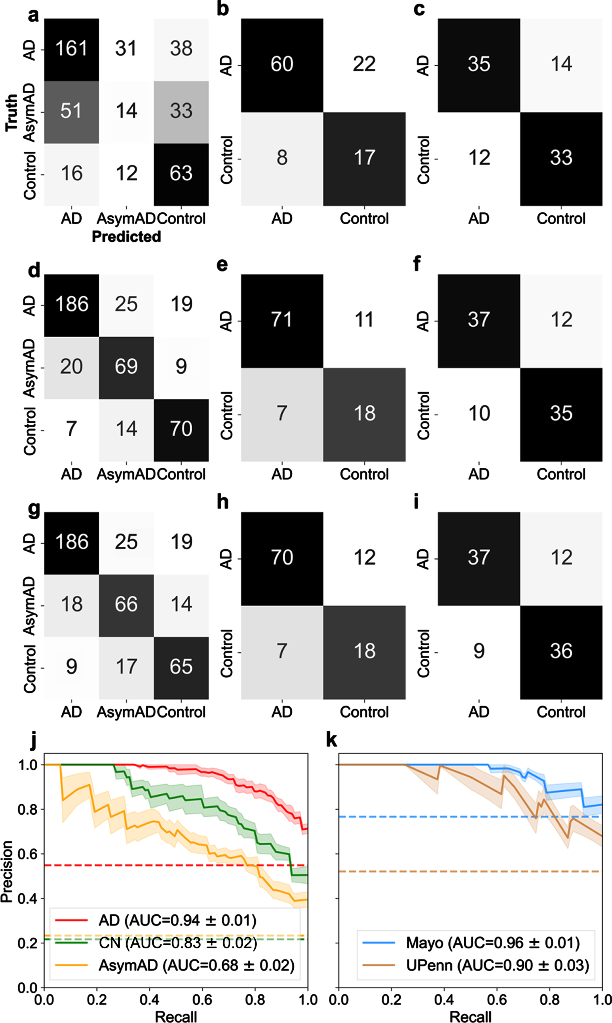
A precision-recall (PR) curve curve is used to assess aggregate classifier performance. AUC is used to quantify the aggregate classification performance using the selected best protein subset(s). AUC = 1 is a perfect classifier; thus, an AUC closer to 1 is desirable. Figure 2j illustrates the PR curve and corresponding AUC for the protein selection cohort for AD, control, and AsymAD, respectively, using the selected 29 best proteins. The shaded area represents the standard error, ±σ. The 29 best proteins do well in correctly classifying AD (AUC = 0.94±0.01; shown in red in Fig. 2j) and control (AUC = 0.83±0.02; shown in green in Fig. 2j). However, the best 29 proteins are poor at classifying AsymAD (AUC = 0.68±0.02; shown in yellow in Fig. 2j). Figure 2k illustrates the PR curve and corresponding AUC for the independent validation cohorts of Mayo and UPenn, respectively. The AUC for Mayo cohort was 0.96±0.01 whereas the UPenn cohort AUC was 0.90±0.03. Thus, the model performed equally well in diagnosing unseen AD and Control patients in both independent validation cohorts with the 29-protein subset. The fact validation data originated from different brain regions provides further confidence that the 29-protein subset model is generalizable to other future data sets. The selected proteins do not have a high degree of correlation between them, which supports that the predictive ability does not rest upon a few proteins in the set (Supplementary Figure 3). Moreover, the unsupervised clustering method, t-SNE, illustrated good separability of the AD, AsymAD, and control classes using the selected subset of 29 “best” proteins (Supplementary Figure 4).
The best 29 proteins are listed in Fig. 3a with their corresponding model coefficient weight as determined from the SVM classification model. Since the one-versus-rest approach for multi-class classification is used, it results in three coefficients for each protein. The three coefficients for every protein correspond to the three diagnostic classes (AD, AsymAD, and Control). The corresponding heatmap illustrates how the selected proteins (n = 29) drive classification of AD, AsymAD, or Control. Purple represents negative drivers and blue positive drivers. The depth of the hue corresponds to relative magnitude of the coefficient as shown on the heatmap coefficient scale in Fig. 3a. For example, increased APP strongly drives up AD classification, strongly drives down Control, and slightly drives up AsymAD. Similar interpretations can be made for all proteins and their effect on each class.
Fig. 3
Driving effects of the selected 29 proteins on the prediction of diagnostic classes of Alzheimer’s (AD), asymptomatic Alzheimer’s (AsymAD), and Control. Note the color of the box around individual listed proteins corresponds to functional modules derived in Johnson et al. [3] and detailed later in Fig. 6. a) The heatmap illustrates the relative magnitude that each protein drives diagnostic class. Driving effects are determined from the coefficients of the SVM. Since the one-versus-rest approach for multi-class classification is used, results encompass three coefficients for each selected protein, one coefficient corresponding to each diagnostic class (AD, AsymAD, Control). b) Key proteins that drive correct prediction in multiple or overlapping classes. The Venn diagram illustrates the overlap in classes: area 1 denotes overlap between AD and Control, area 2 overlap between AD and AsymAD and area 3 between AsymAD and Control. The biomarker panels for each overlap area denote individual predictive proteins shared by overlapping classes.
![Driving effects of the selected 29 proteins on the prediction of diagnostic classes of Alzheimer’s (AD), asymptomatic Alzheimer’s (AsymAD), and Control. Note the color of the box around individual listed proteins corresponds to functional modules derived in Johnson et al. [3] and detailed later in Fig. 6. a) The heatmap illustrates the relative magnitude that each protein drives diagnostic class. Driving effects are determined from the coefficients of the SVM. Since the one-versus-rest approach for multi-class classification is used, results encompass three coefficients for each selected protein, one coefficient corresponding to each diagnostic class (AD, AsymAD, Control). b) Key proteins that drive correct prediction in multiple or overlapping classes. The Venn diagram illustrates the overlap in classes: area 1 denotes overlap between AD and Control, area 2 overlap between AD and AsymAD and area 3 between AsymAD and Control. The biomarker panels for each overlap area denote individual predictive proteins shared by overlapping classes.](https://content.iospress.com:443/media/jad/2023/92-2/jad-92-2-jad220683/jad-92-jad220683-g003.jpg)
Figure 3b examines the overlap of the 29 selected proteins in driving diagnostic class (AD, AsymAD, Control). AD and Control, labeled as area 1 on the Venn diagram, share 7 driving proteins: APP, DHX15, NRXN1, PBXIP1, RABEP1, STOM, and VGF. AD and AsymAD, labeled as area 2 on the Venn diagram, share eight driving proteins: ALDH1A1, BDH2, C4A, FABP7, GABBR2, GNAI3, PBXIP1, PKAR1B. AsymAD and Control, labeled as area 3 on the Venn diagram, share seven driving proteins: APP, C4A, DMXL1, EXOC2, PITPNB, RABEP1, and VGF. Note that the color coding of each protein, itself, in Fig. 3 corresponds to function as described in the Functional Themes in the Selected Proteins section. The most predictive proteins tend to have opposite signs for coefficient modulation between discriminatory class pairs (AD and control; AD and AsymAD; and AsymAD and Control).
Classification performance with 88 proteins
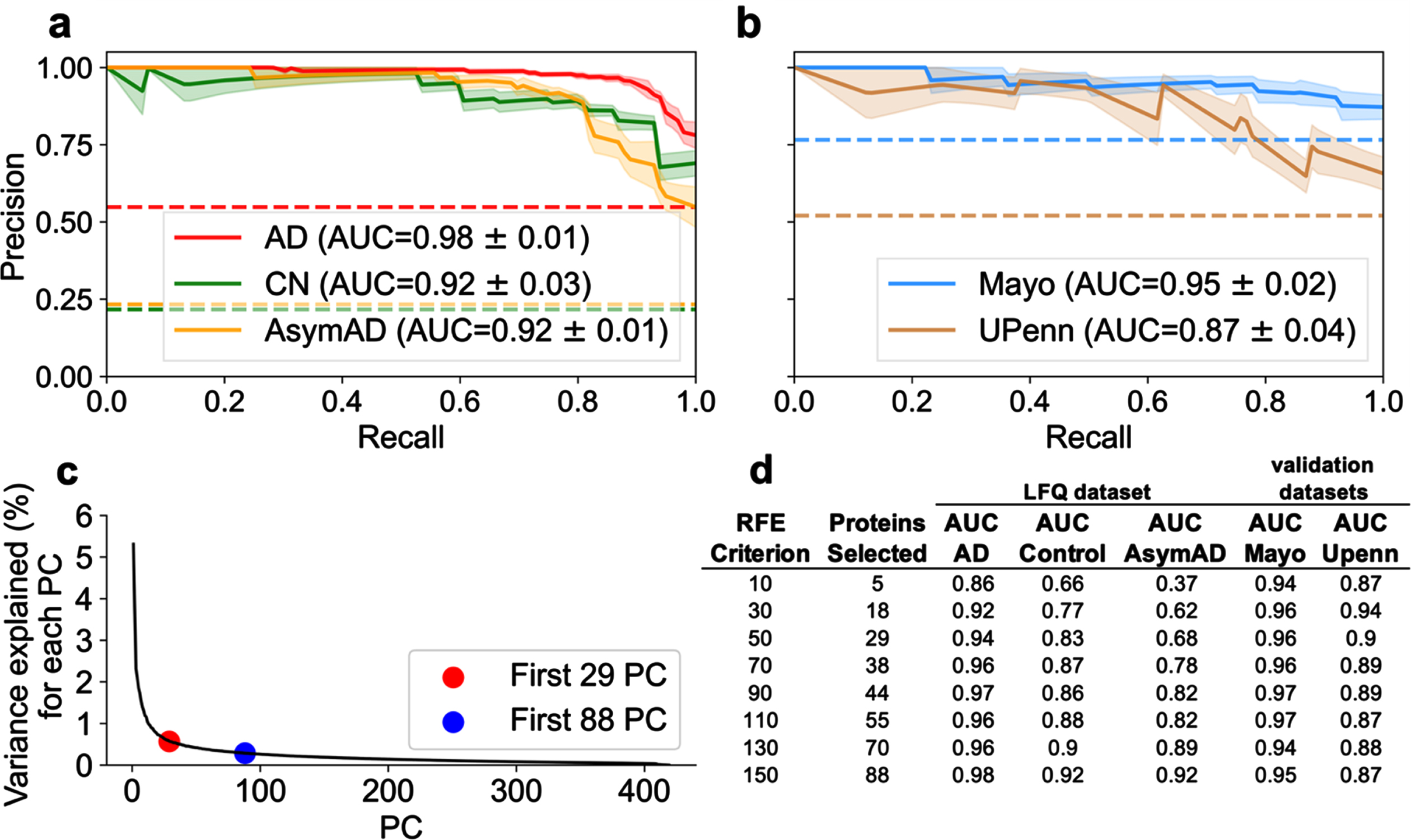
An RFE of 50, resulting in 29 selected proteins, was sufficient for differentiating AD and Control classes. However, an RFE criterion of 150, resulting in 88 selected proteins, was optimal for differentiating AD and AsymAD classes. Figure 4a and 4b illustrate the PR curve and AUC for each class utilizing the 88 protein subset for predicting diagnostic classification. Utilizing the 88-protein subset increased AD and Control classification performance by approximately 4% and 9% respectively compared to the 29-protein subset (Fig. 4a). Utilizing the 88-protein subset increased AsymAD classification performance by approximately 24% (Fig. 4a). In the independent validation cohorts (Fig. 4b), which did not contain any AsymAD patients, the 29-protein subset marginally outperformed the 88-protein subset. In short, AsymAD requires substantially more proteins for accurate predictive classification.
Fig. 4
Examination of optimal number of proteins necessary for superior classification between AD, AsymAD, and Control. A best predictive protein set of 88 (n = 88 proteins) was determined to ensure accurate discrimination between AD, AsymAD and Controls in the LFQ dataset. This was based on an assessment of the RFE criterion, principal component analysis (PCA), and evaluation of classifier using area under the curve (AUC) with standard error (±σ). a) AUC of the precision-recall curve for classification of AD, AsymAD, Control using the n = 88 best predictive protein set. b) AUC of the precision-recall curve for classification of Control versus AD using the n = 88 proteins in the Mayo and UPenn datasets. Of the 88, Mayo dataset had 77 and UPenn dataset had 63 proteins respectively. c) PCA examining variance explained versus number of principal components. Red dot corresponds to the n = 29 selected protein subset and blue dot to the n = 88 selected protein subset. The “elbow” of the scree plot ends by about 88 principal components. d) Analysis of impact of RFE criterion and resultant number of selected best predictive proteins in the LFQ dataset and the validation datasets using each respective resultant protein subset for classification.
Further exploration of classification performance as a function of RFE criterion
The RFE criterion for protein selection was varied to determine the optimal protein subsets. Again, the RFE criterion determines the number of proteins each classifier (SVM and LR) can select. For a given RFE criterion, the intersection of proteins selected by both SVM and LR become the resultant number of “best” predictive proteins. As described above, RFE = 50, resulting in 29 proteins, was sufficient to classify AD versus control. The number of intersecting best predictive proteins for diagnostic classification is not random. Rather, these thresholds are explained by examining dimensional reduction with PCA. Figure 4c illustrates variance explained as a function of number of components. The scree plot approximates minimum components needed to explain the preponderance of variance. The “elbow” of the scree plot denotes the optimal range of components needed to account for the preponderance of variance. Figure 4c shows 29 components (red dot) corresponds to the start of the elbow and 88 components (black dot) corresponds to the end of the elbow. Variance per component beyond the elbow asymptotically approaches zero. Hence, those additional components should not substantively improve model performance. Figure 4d examines the impact of RFE criterion and the resultant number of selected best predictive proteins on diagnostic classification performance. Selecting a RFE criterion greater than 150 (not shown) did not result in increased classification performance.
Functional themes in the selected proteins
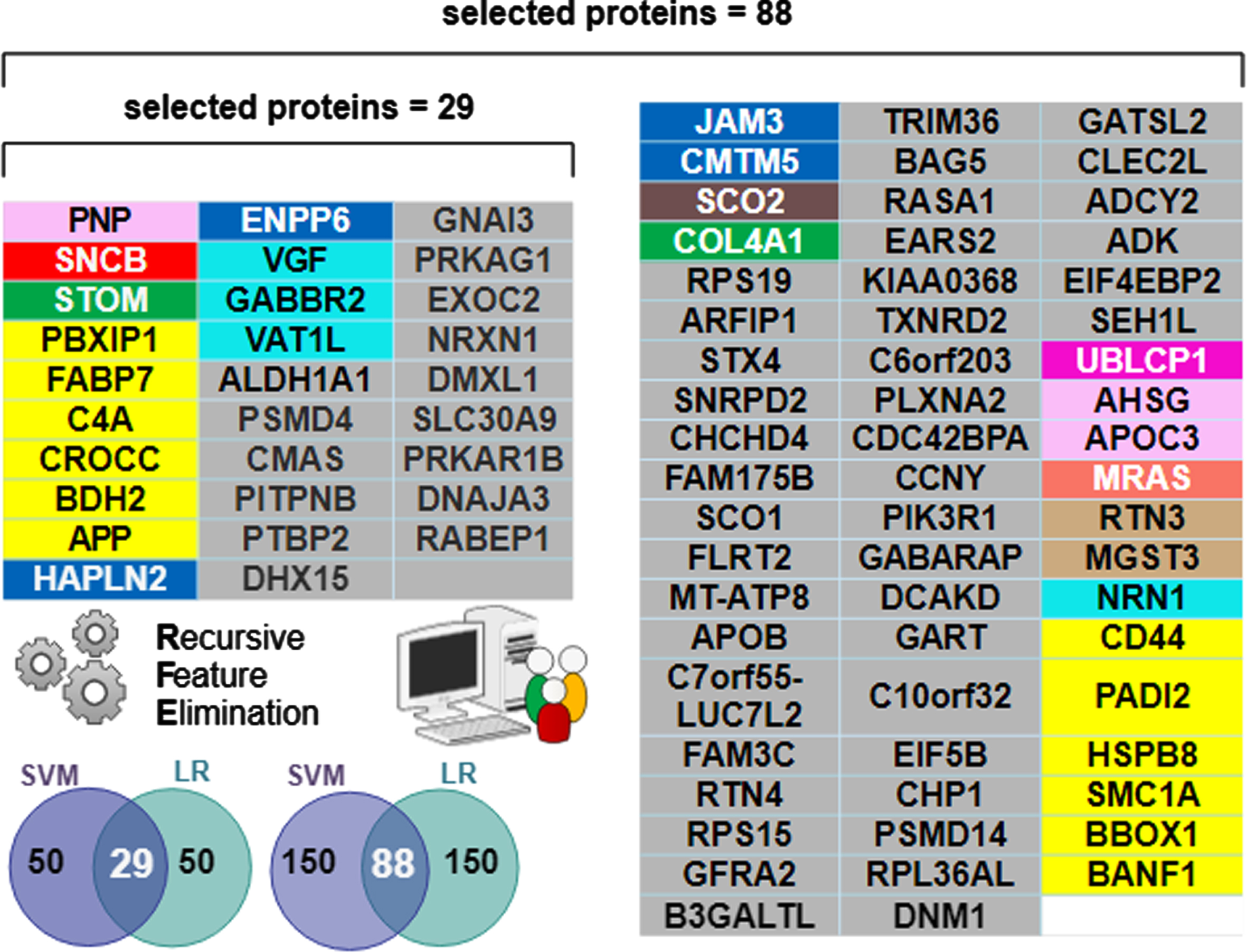
The biomarker proteins were mapped to their corresponding modules, which were identified by using the weighted gene correlation network analysis (WGCNA) algorithm. Colors and module number are used to define the function of the biomarkers [3] and are recapitulated in the first 3 columns of Fig. 5. Functional module frequency (expressed as a percentage) of selected best proteins (for n = 29 and n = 88) were compared to the source frequency for the total protein set (n = 3,334). Change in frequency of selected protein module compared to source frequency is indicative of relative importance of a functional module in predicting diagnostic class (AD, AsymAD, Control). The most enriched module in selected protein sets for both n = 29 and n = 88 corresponds to sugar metabolism. Sugar metabolism (M4, yellow) most strongly correlated with AD associated traits (cognition r = –0.67, p = 8.5×10⁻²³; neurofibrillary tangle r = 0.49, p = 4.7×10⁻²⁷; amyloid-β plaque r = 0.46, p = 1.3×10⁻²³ and functional status r = 0.52, p = 2.6×10⁻¹²), as reported in [3]. The 29 best proteins are significantly (p < 0.05) enriched with the sugar metabolism module (M4, yellow). Proteins belonging to sugar metabolism (M4) constituted 5.6% of 3334 total proteins analyzed. However, sugar metabolism proteins constituted 20.7% of the selected best 29 proteins and 13.6% of the selected best 88 proteins (Fig. 5). The remaining functional modules are not significantly different in their representation in either set of selected best proteins. Figure 6 lists the individually selected 29 best proteins (n = 29) and 88 best proteins (n = 88) color-coded by functional module. Note the 29-protein set is a subset of the 88-protein set (e.g., the best 29 proteins are all present within the best 88 proteins).
Fig. 5
Functional Protein Module of Selected “Best” Predictive Proteins. The functional protein modules are as defined by Johnson et al. [3]. Source frequency is the frequency of the module in the source protein set (n = 3334 unique proteins). The selected frequency is for selected best proteins, n = 29 or n = 88. The M4 yellow module for sugar metabolism is significantly enriched (p < 0.05) in selected proteins compared to their frequency in source. Enrichment of sugar metabolism in the selected predictive proteins signifies their importance to diagnostic classification.
![Functional Protein Module of Selected “Best” Predictive Proteins. The functional protein modules are as defined by Johnson et al. [3]. Source frequency is the frequency of the module in the source protein set (n = 3334 unique proteins). The selected frequency is for selected best proteins, n = 29 or n = 88. The M4 yellow module for sugar metabolism is significantly enriched (p < 0.05) in selected proteins compared to their frequency in source. Enrichment of sugar metabolism in the selected predictive proteins signifies their importance to diagnostic classification.](https://content.iospress.com:443/media/jad/2023/92-2/jad-92-2-jad220683/jad-92-jad220683-g005.jpg)
DISCUSSION
Of the 3,334 proteins, machine learning determined a minimum 29-protein subset necessary to accurately classify AD and Control, but an 88-protein subset was necessary to accurately classify AsymAD. The additional proteins needed for AsymAD classification is likely due to greater complexity and heterogeneity of the AsymAD disease state. The “best” predictive protein subsets (n = 29 and n = 88) were significantly enriched for sugar metabolism (Fig. 6).
Fig. 6
Individual proteins comprising the selected “best” predictive protein subsets color-coded by functional module. The n = 29 subset was sufficient for differentiating AD from Control. However, the n = 88 subset was optimal for differentiating AD and AsymAD. Note all 29 proteins in the n = 29 selected set are contained within the n = 88 selected set. The Venn diagram inset pictorially summarizes the Recursive Feature Elimination (RFE) algorithm used to select the best protein subsets. The intersecting predictive proteins selected by both the support vector machine (SVM) and logistic regression (LR) classifiers during RFE became the “best proteins”. A RFE criterion = 50 resulted in 29 best proteins (e.g., intersection shown on the left Venn inset). A RFE criterion = 150 resulted in 88 best proteins (intersection shown on the right Venn inset).
Homeostatic regulatory dynamics key to disease progression
There was relatively little overlap between the predictive proteins that drive control-AsymAD changes and predictive proteins that drive AsymAD-AD changes (see Fig. 3b). This finding indicates an associative relationship to multifactorial dynamic disease progression etiology. In short, the most predictive proteins dynamically change with disease stage (see Fig. 3a). Whether familial or sporadic AD, different underlying proteomic perturbations may result in multi-scalar system destabilization (e.g., failed homeostasis) with corresponding functional disease phenotypes. Homeostasis is critical for maintaining health, and thus, instabilities often appear in disease [17]. Multifactorial homeostatic instability has been suggested as an underlying propagating mechanism in other neurological pathology, including amyotrophic lateral sclerosis [18], absence epileptic seizures [19], Parkinson’s disease [20], and secondary spinal cord injury [21].
Overlapping proteins for class discrimination
Supplementary Table 1 presents literature details on functions and cited associations with each member of the 29-protein subset. Supplementary Table 1 includes the protein unique ID, brief description of its function and role in AD (if known), and a corresponding reference. Five proteins of the 29-protein subset overlapped in class discrimination (Fig. 3b): APP, VGF, RABEP1, C4A, PBXIP1. APP (upregulated in AD, AsymAD) was expected given its role in the amyloid cascade [16]. VGF (downregulated in AD) protects against amyloid-β pathology [22]. RABEP1 was key for differentiating Control (upregulated) from AD or AsymAD (downregulated). RABEP1 is tied to longevity and AD [23]. C4A was key for differentiating AsymAD (downregulated) from AD (upregulated) or Control. Increased C4A copy number [24] impacts AD risk and schizophrenia [25]. PBXIP1 was key for differentiating AD (upregulated) from AsymAD (downregulated) or Control. PBXIP1 is cited as altering cell viability and motility through rearrangements of the actin cytoskeleton [26]. Interestingly, many of the 29-proteins are also biomarkers for various non-neural cancers.
Sugar metabolism biomarkers enriched in 29-protein and 88-protein set
Sugar metabolism proteins in both the 29-protein and 88-protein sets (Fig. 6) included: APP, BDH2, C4A, CROCC, FABP7, PBXIP1. Sugar metabolism proteins in the expanded 88-protein subset included CD44, an immune marker associated with AD [27]; PADI2, an age and AD-related marker [28]; BANF1, implicated in aging and progeria [29]; HSPB8, inhibitor of amyloid-β formation [30]; SMC1A, where increased copy number is implicated in epilepsy, AD, and other neurodegenerative diseases [31]; BBOX1, implicated in diabetic kidney disease, lipid metabolic disorders, and schizophrenia [32].
The significantly enriched sugar metabolism module (Fig. 5) supports the recent perspective that asymptomatic and symptomatic AD is characterized by dysregulation of energy metabolism [33, 34]. In short, the presented work supports the hypothesis that sugar metabolism becomes more impacted with disease progression. Insulin resistance in the brain modulates AD inflammatory markers and decreases amyloid clearance [35]. The exact link between AD and type 1 or 2 diabetes is under debate. Nonetheless, poorly controlled blood sugar appears to increase risk of AD [35]. Some researchers have referred to the dysregulation of blood sugar in the brain in AD “type 3 diabetes” [36]. Interconnections between inflammation, metabolism, and protein clearance are further evidence of a multifactorial homeostatic instability contributing to AD progression [3, 10, 34, 37].
The good and the bad of APP
APP is another example where homeostatic instability may play a role in disease progression. For quite some time, APP has been known to be involved in the formation of amyloid-β. A recent genome-wide association study identified APP as a relevant pathway in both familial and sporadic AD [38]. Typically, APP is associated with the formation of toxic soluble amyloid-β oligomers. However, researchers have also suggested that the production of soluble APP alpha (sAPPα) may be a compensatory mechanism to help stave off AD pathology [39]. In particular, amyloid-β monomers have similar neuroprotective properties as sAPPα; they are neurotrophic and neuroprotective and enhance neurogenesis. Hence, deciphering the possible neuroprotective versus the neurogenic role of APP in AD is an ongoing area of research [40]. The present study cannot confirm or deny the precise causal role of APP as protective, destructive, or a combination of both. The present study’s association-based results do show that APP is an important diagnostic classifier in disambiguating the three stages (Control, AsymAD, AD), as shown in Fig. 3. Nonetheless, the diagnostic classification ability of APP is complex and intertwined with other biomarkers (Fig. 2d-f). When APP was used alone without any other biomarkers, it was not a good classifier (Fig. 2a-c), especially for AsymAD.
Blood-based biomarkers
Biomarkers detected in the blood are preferable for AD risk assessment and early diagnosis [41]. Only one blood-based module protein was selected in the 29-protein subset: PNP, a purine-related metabolite altered early in AD [42]. Two additional blood-based proteins were in the 88-protein subset: AHSG and APOC3. A higher apoE level in high density lipoprotein that lacks apoC3 was associated with better cognitive function [43]. AHSG, a highly glycosylated protein appears downregulated in AD [44].
Assessment of alternatives and limitations
The presented RFE method in Fig. 1, and its corresponding presented results above, were thoroughly vetted and compared to several other statistics-based and machine learning-based model alternatives. The presented method consistently outperformed all other alternative methods and models (see Supplementary Figures 5–8), especially in the mega-LFQ data set with three classes (Control, AsymAD, and AD). In summary, the presented 29-protein and 88-protein lists for diagnostic classification were quite stable. Relaxing the RFE criterion to include more proteins beyond the selected 88-proteins did not improve classification results (Fig. 4). Nonetheless, no model or method is perfect. While the model is stable, it is fair to expect that a small number of proteins included on the final presented list(s) could be substituted for non-included proteins (e.g., such as similarly co-expressed proteins or proteins from the same functional module). As such, regardless of method, a few proteins that relayed similar, correlated, or mutual information as the selected proteins may not have made the presented final selected proteins list(s). In full transparency, the performance of the protein list generated by each alternative method is shown in Supplementary Figures 5–8. Notably, many of the RFE selected final proteins presented in the main article were recurringly selected by the alternative methods. Finally, any proteins not included in the presented final lists (or even in the input study data) could have their relative importance deduced based on co-expression or their functional modules.
Future directions
The LFQ data covered 3,334 proteins from which the identified “best” biomarker subset is derived. However, the presented method could be extended to future more comprehensive data sets, such as tandem mass tag, to further optimize results. Future addition of larger validation cohorts, especially AsymAD, will ensure model generalizability. Additionally, future inclusion of traits such as gender and race (when available) are important to determine if there are specific feature biases that impact the predictive ability or discriminative expression of proteins. Finally, this work utilized the common 3-class AD staging system: control, AsymAD, or AD. However, it is possible there is a more optimal temporal disease staging system. For example, integrative data machine learning analysis suggested with Alzheimer’s Disease Neuroimaging Initiative data suggested at least four clusters of symptomatic AD patients [45].
Conclusions
Machine learning successfully identified proteins subsets most predictive for classifying AD, AsymAD, and Control subjects. The most predictive proteins subsets comprised < 3% of the 3,334 proteins assessed. A 29-protein subset accurately classified AD versus Control, but an 88-protein subset was needed to accurately classify AsymAD. The protein subsets resulted in a robust classifier model. The presented model generalized to accurately predict diagnostic labels on unseen data in independent validation cohorts regardless of brain region or minor data set differences. The predictive protein subsets included known important proteins like APP. However, diagnostic classification performance did not hinge upon APP or any single protein or pathway. Finally, the most predictive subsets were significantly enriched in proteins linked to sugarmetabolism.
ACKNOWLEDGMENTS
The authors have no acknowledgments to report.
FUNDING
This research was funded by National Science Foundation CAREER grant 1944247 to C.M, Alzheimer’s Association Research Grant Award 2018-AARGD-591014 to C.M., Goizueta Alzheimer’s Disease Research Center at Emory University grant awards P50 AG025688 and P30 AG066511 to C.M., National Institute of Health grant U19-AG056169 sub-awards to C.M, J.L., A.L.
CONFLICT OF INTEREST
C.M. is an Editorial Board Member of this journal but was not involved in the peer-review process nor had access to any information regarding its peer-review.
DATA AVAILABILITY
All data used in the analysis has been previously published in [3] and is publicly available at https://www.synapse.org/#!Synapse:syn20933797/files/.
SUPPLEMENTARY MATERIAL
[1] The supplementary material is available in the electronic version of this article: https://dx.doi.org/10.3233/JAD-220683.
REFERENCES
[1] | Singh M , Singh SP , Dubey PK , Rachana R , Mani S , Yadav D , Agarwal M , Agarwal S , Agarwal V , Kaur H ((2020) ) Advent of proteomic tools for diagnostic biomarker analysis in Alzheimer’s disease. Curr Protein Pept Sci 21: , 965–977. |
[2] | Wang M , Beckmann ND , Roussos P , Wang E , Zhou X , Wang Q , Ming C , Neff R , Ma W , Fullard JF , Hauberg ME , Bendl J , Peters MA , Logsdon B , Wang P , Mahajan M , Mangravite LM , Dammer EB , Duong DM , Lah JJ , Seyfried NT , Levey AI , Buxbaum JD , Ehrlich M , Gandy S , Katsel P , Haroutunian V , Schadt E , Zhang B ((2018) ) The Mount Sinai cohort of large-scale genomic, transcriptomic and proteomic data in Alzheimer’s disease. Sci Data 5: , 180185. |
[3] | Johnson ECB , Dammer EB , Duong DM , Ping L , Zhou M , Yin L , Higginbotham LA , Guajardo A , White B , Troncoso JC , Thambisetty M , Montine TJ , Lee EB , Trojanowski JQ , Beach TG , Reiman EM , Haroutunian V , Wang M , Schadt E , Zhang B , Dickson DW , Ertekin-Taner N , Golde TE , Petyuk VA , De Jager PL , Bennett DA , Wingo TS , Rangaraju S , Hajjar I , Shulman JM , Lah JJ , Levey AI , Seyfried NT ((2020) ) Large-scale proteomic analysis of Alzheimer’s disease brain and cerebrospinal fluid reveals early changes in energy metabolism associated with microglia and astrocyte activation. Nat Med 26: , 769–780. |
[4] | Wolfsgruber S , Jessen F , Wiese B , Stein J , Bickel H , Mosch E , Weyerer S , Werle J , Pentzek M , Fuchs A , Kohler M , Bachmann C , Riedel-Heller SG , Scherer M , Maier W , Wagner M , AgeCoDe Study G ((2014) ) The CERAD neuropsychological assessment battery total score detects and predicts Alzheimer disease dementia with high diagnostic accuracy. Am J Geriatr Psychiatry 22: , 1017–1028. |
[5] | Iacono D , Resnick SM , O’Brien R , Zonderman AB , An Y , Pletnikova O , Rudow G , Crain B , Troncoso JC ((2014) ) Mild cognitive impairment and asymptomatic Alzheimer disease subjects: Equivalent beta-amyloid and tau loads with divergent cognitive outcomes. J Neuropathol Exp Neurol 73: , 295–304. |
[6] | Watson Y , Nelson B , Kluesner JH , Tanzy C , Ramesh S , Patel Z , Kluesner KH , Singh A , Murthy V , Mitchell CS ((2021) ) Aggregate trends of apolipoprotein E on cognition in transgenic Alzheimer’s disease mice. J Alzheimers Dis 83: , 435–450. |
[7] | Huber CM , Yee C , May T , Dhanala A , Mitchell CS ((2018) ) Cognitive decline in preclinical Alzheimer’s disease: Amyloid-beta versus tauopathy. J Alzheimers Dis 61: , 265–281. |
[8] | Hammond TC , Xing X , Wang C , Ma D , Nho K , Crane PK , Elahi F , Ziegler DA , Liang G , Cheng Q , Yanckello LM , Jacobs N , Lin AL ((2020) ) beta-amyloid and tau drive early Alzheimer’s disease decline while glucose hypometabolism drives late decline. Commun Biol 3: , 352. |
[9] | Foley AM , Ammar ZM , Lee RH , Mitchell CS ((2015) ) Systematic review of the relationship between amyloid-beta levels and measures of transgenic mouse cognitive deficit in Alzheimer’s disease. J Alzheimers Dis 44: , 787–795. |
[10] | Jaaskelainen O , Hall A , Tiainen M , van Gils M , Lotjonen J , Kangas AJ , Helisalmi S , Pikkarainen M , Hallikainen M , Koivisto A , Hartikainen P , Hiltunen M , Ala-Korpela M , Soininen P , Soininen H , Herukka SK ((2020) ) Metabolic profiles help discriminate mild cognitive impairment from dementia stage in Alzheimer’s disease. J Alzheimers Dis 74: , 277–286. |
[11] | Gaetani L , Bellomo G , Parnetti L , Blennow K , Zetterberg H , Di Filippo M ((2021) ) Neuroinflammation and Alzheimer’s disease: A machine learning approach to CSF proteomics. Cells 10: , 1930. |
[12] | O’Brien RJ , Resnick SM , Zonderman AB , Ferrucci L , Crain BJ , Pletnikova O , Rudow G , Iacono D , Riudavets MA , Driscoll I , Price DL , Martin LJ , Troncoso JC ((2009) ) Neuropathologic studies of the Baltimore Longitudinal Study of Aging (BLSA). J Alzheimers Dis 18: , 665–675. |
[13] | Beach TG , Adler CH , Sue LI , Serrano G , Shill HA , Walker DG , Lue L , Roher AE , Dugger BN , Maarouf C , Birdsill AC , Intorcia A , Saxon-Labelle M , Pullen J , Scroggins A , Filon J , Scott S , Hoffman B , Garcia A , Caviness JN , Hentz JG , Driver-Dunckley E , Jacobson SA , Davis KJ , Belden CM , Long KE , Malek-Ahmadi M , Powell JJ , Gale LD , Nicholson LR , Caselli RJ , Woodruff BK , Rapscak SZ , Ahern GL , Shi J , Burke AD , Reiman EM , Sabbagh MN ((2015) ) Arizona Study of Aging and Neurodegenerative Disorders and Brain and Body Donation Program. Neuropathology 35: , 354–389. |
[14] | Guyon I , Weston J , Barnhill S , Vapnik V ((2002) ) Gene selection for cancer classification using support vector machines. Mach Learn 46: , 389–422. |
[15] | Pedregosa F , Varoquaux G , Gramfort A , Michel V , Thirion B , Grisel O , Blondel M , Prettenhofer P , Weiss R , Dubourg V , Vanderplas J , Passos A , Cournapeau, D , Brucher M , Perrot M , Duchesnay E ((2011) ) Scikit-learn: Machine Learning in Python. J Mach Learn Res 12: , 2825–2830. |
[16] | Hardy J ((2017) ) The discovery of Alzheimer-causing mutations in the APP gene and the formulation of the “amyloid cascade hypothesis". FEBS J 284: , 1040–1044. |
[17] | Billman GE ((2020) ) Homeostasis: The underappreciated and far too often ignored central organizing principle of physiology. Front Physiol 11: , 200. |
[18] | Irvin CW , Kim RB , Mitchell CS ((2015) ) Seeking homeostasis: Temporal trends in respiration, oxidation, and calcium in SOD1 G93A amyotrophic lateral sclerosis mice. Front Cell Neurosci 9: , 248. |
[19] | Gillary G , Niebur E ((2016) ) The edge of stability: Response times and delta oscillations in balanced networks. PLoS Comput Biol 12: , e1005121. |
[20] | McAuley JH , Marsden CD ((2000) ) Physiological and pathological tremors and rhythmic central motor control. Brain 123 (Pt 8): , 1545–1567. |
[21] | Mitchell CS , Lee RH ((2008) ) Pathology dynamics predict spinal cord injury therapeutic success. J Neurotrauma 25: , 1483–1497. |
[22] | Beckmann ND , Lin WJ , Wang M , Cohain AT , Charney AW , Wang P , Ma W , Wang YC , Jiang C , Audrain M , Comella PH , Fakira AK , Hariharan SP , Belbin GM , Girdhar K , Levey AI , Seyfried NT , Dammer EB , Duong D , Lah JJ , Haure-Mirande JV , Shackleton B , Fanutza T , Blitzer R , Kenny E , Zhu J , Haroutunian V , Katsel P , Gandy S , Tu Z , Ehrlich ME , Zhang B , Salton SR , Schadt EE ((2020) ) Multiscale causal networks identify VGF as a key regulator of Alzheimer’s disease. Nat Commun 11: , 3942. |
[23] | Miller JB , Ward E , Staley LA , Stevens J , Teerlink CC , Tavana JP , Cloward M , Page M , Dayton L ; Alzheimer’s Disease Genetics Consortium; Cannon-Albright LA , Kauwe JS ((2020) ) Identification and genomic analysis of pedigrees with exceptional longevity identifies candidate rare variants. Neurobiol Dis 143: , 104972. |
[24] | Zorzetto M , Datturi F , Divizia L , Pistono C , Campo I , De Silvestri A , Cuccia M , Ricevuti G ((2017) ) Complement C4A and C4B gene copy number study in Alzheimer’s disease patients. Curr Alzheimer Res 14: , 303–308. |
[25] | Yilmaz M , Yalcin E , Presumey J , Aw E , Ma M , Whelan CW , Stevens B , McCarroll SA , Carroll MC ((2021) ) Over-expression of schizophrenia susceptibility factor human complement C4A promotes excessive synaptic loss and behavioral changes in mice. Nat Neurosci 24: , 214–224. |
[26] | van Vuurden DG , Aronica E , Hulleman E , Wedekind LE , Biesmans D , Malekzadeh A , Bugiani M , Geerts D , Noske DP , Vandertop WP , Kaspers GJ , Cloos J , Wurdinger T , van der Stoop PP ((2014) ) Pre-B-cell leukemia homeobox interacting protein 1 is overexpressed in astrocytoma and promotes tumor cell growth and migration. Neuro Oncol 16: , 946–959. |
[27] | Rangaraju S , Dammer EB , Raza SA , Rathakrishnan P , Xiao H , Gao T , Duong DM , Pennington MW , Lah JJ , Seyfried NT , Levey AI ((2018) ) Identification and therapeutic modulation of a pro-inflammatory subset of disease-associated-microglia in Alzheimer’s disease. Mol Neurodegener 13: , 24. |
[28] | Yu L , Dawe RJ , Boyle PA , Gaiteri C , Yang J , Buchman AS , Schneider JA , Arfanakis K , De Jager PL , Bennett DA ((2017) ) Association between brain gene expression, DNA methylation, and alteration of ex vivo magnetic resonance imaging transverse relaxation in late-life cognitive decline. JAMA Neurol 74: , 1473–1480. |
[29] | Osorio FG , Ugalde AP , Marino G , Puente XS , Freije JM , Lopez-Otin C ((2011) ) Cell autonomous and systemic factors in progeria development. Biochem Soc Trans 39: , 1710–1714. |
[30] | Wilhelmus MM , Boelens WC , Otte-Holler I , Kamps B , Kusters B , Maat-Schieman ML , de Waal RM , Verbeek MM ((2006) ) Small heat shock protein HspB8: Its distribution in Alzheimer’s disease brains and its inhibition of amyloid-beta protein aggregation and cerebrovascular amyloid-beta toxicity. Acta Neuropathol 111: , 139–149. |
[31] | Yan J , Zhang F , Brundage E , Scheuerle A , Lanpher B , Erickson RP , Powis Z , Robinson HB , Trapane PL , Stachiw-Hietpas D , Keppler-Noreuil KM , Lalani SR , Sahoo T , Chinault AC , Patel A , Cheung SW , Lupski JR ((2009) ) Genomic duplication resulting in increased copy number of genes encoding the sister chromatid cohesion complex conveys clinical consequences distinct from Cornelia de Lange. J Med Genet 46: , 626–634. |
[32] | Rigault C , Le Borgne F , Demarquoy J ((2006) ) Genomic structure, alternative maturation and tissue expression of the human BBOX1 gene. Biochim Biophys Acta 1761: , 1469–1481. |
[33] | Ryu WI , Bormann MK , Shen M , Kim D , Forester B , Park Y , So J , Seo H , Sonntag KC , Cohen BM ((2021) ) Brain cells derived from Alzheimer’s disease patients have multiple specific innate abnormalities in energy metabolism. Mol Psychiatry 26: , 5702–5714. |
[34] | Yang Z , Wang J , Chen J , Luo M , Xie Q , Rong Y , Wu Y , Cao Z , Liu Y ((2022) ) High-resolution NMR metabolomics of patients with subjective cognitive decline plus: Perturbations in the metabolism of glucose and branched-chain amino acids. Neurobiol Dis 171: , 105782. |
[35] | Tumminia A , Vinciguerra F , Parisi M , Frittitta L ((2018) ) Type 2 diabetes mellitus and Alzheimer’s disease: Role of insulin signalling and therapeutic implications. Int J Mol Sci 19: , 3306. |
[36] | Nguyen TT , Ta QTH , Nguyen TKO , Nguyen TTD , Giau VV ((2020) ) Type 3 diabetes and its role implications in Alzheimer’s disease. Int J Mol Sci 21: , 3165. |
[37] | Yilmaz A , Ustun I , Ugur Z , Akyol S , Hu WT , Fiandaca MS , Mapstone M , Federoff H , Maddens M , Graham SF ((2020) ) A community-based study identifying metabolic biomarkers of mild cognitive impairment and Alzheimer’s disease using artificial intelligence and machine learning. J Alzheimers Dis 78: , 1381–1392. |
[38] | Bellenguez C , Kucukali F , Jansen IE , Kleineidam L , Moreno-Grau S , Amin N , Naj AC , Campos-Martin R , Grenier-Boley B , Andrade V , et al. ((2022) ) New insights into the genetic etiology of Alzheimer’s disease and related dementias. Nat Genet 54: , 412–436. |
[39] | Chasseigneaux S , Allinquant B ((2012) ) Functions of Abeta, sAPPalpha and sAPPbeta: Similarities and differences. J Neurochem 120: (Suppl 1), 99–108. |
[40] | Dar NJ , Glazner GW ((2020) ) Deciphering the neuroprotective and neurogenic potential of soluble amyloid precursor protein alpha (sAPPalpha). Cell Mol Life Sci 77: , 2315–2330. |
[41] | Eke CS , Jammeh E , Li X , Carroll C , Pearson S , Ifeachor E ((2021) ) Early detection of Alzheimer’s disease with blood plasma proteins using support vector machines. IEEE J Biomed Health Inform 25: , 218–226. |
[42] | Alonso-Andres P , Albasanz JL , Ferrer I , Martin M ((2018) ) Purine-related metabolites and their converting enzymes are altered in frontal, parietal and temporal cortex at early stages of Alzheimer’s disease pathology. Brain Pathol 28: , 933–946. |
[43] | Koch M , DeKosky ST , Goodman M , Sun J , Furtado JD , Fitzpatrick AL , Mackey RH , Cai T , Lopez OL , Kuller LH , Mukamal KJ , Jensen MK ((2020) ) Association of Apolipoprotein E in lipoprotein subspecies with risk of dementia. JAMA Netw Open 3: , e209250. |
[44] | Geroldi D , Minoretti P , Bianchi M , Di Vito C , Reino M , Bertona M , Emanuele E ((2005) ) Genetic association of alpha2-Heremans-Schmid glycoprotein polymorphism with late-onset Alzheimer’s disease in Italians. Neurosci Lett 386: , 176–178. |
[45] | Prakash J , Wang V , Quinn RE 3rd , Mitchell CS ((2021) ) Unsupervised machine learning to identify separable clinical Alzheimer’s disease sub-populations. Brain Sci 11: , 977. |


