
Clustering electricity market participants via FRM models
Abstract
Collateral mechanism in the Electricity Market ensures the payments are executed on a timely manner; thus maintains the continuous cash flow. In order to value collaterals, Takasbank, the authorized central settlement bank, creates segments of the market participants by considering their short-term and long-term debt/credit information arising from all market activities. In this study, the data regarding participants’ daily and monthly debt payment and penalty behaviors is analyzed with the aim of discovering high-risk participants that fail to clear their debts on-time frequently. Different clustering techniques along with different distance metrics are considered to obtain the best clustering. Moreover, data preprocessing techniques along with Recency, Frequency, Monetary Value (RFM) scoring have been used to determine the best representation of the data. The results show that Agglomerative Clustering with cosine distance achieves the best separated clustering when the non-normalized dataset is used; this is also acknowledged by a domain expert.
1.Introduction
Energy Exchange Istanbul (EXIST) – Enerji Piyasaları İşletme Anonim Şirketi (EPİAŞ) was established in 2015 with the aim of managing energy market within the market operation license in an effective, transparent and reliable manner that fulfills the requirements of the energy market. Pursuant to the Electricity Market Balancing and Settlement Regulation (provisional article 19 of the Regulation 27751), Takasbank has been authorized as the central settlement bank to be used by EXIST and market participants for the purpose of operating the collateral mechanism in the Electricity Market and ensuring payments are executed on a timely and accurate manner, and maintaining continuous cash flow in the market. Within the scope of cash clearing and settlement services of Takasbank; market participants perform debt payment transactions, and market receivables are automatically forwarded to the intermediary bank accounts. Within the scope of electricity market collateral management services Takasbank is responsible of managing deposit/withdrawal of collaterals; making margin call to the participants; valuing collaterals and notifying EXIST; and managing interest accrual for the cash collaterals. Takasbank creates the segments of the participants with different risk levels considering their short-term and long-term debt/credit information arising from all the market activities with the aim of identifying high-risk participants. EXIST then utilizes this risk segmentation information to determine the amount of collateral for each participant. This constitutes the motive of this study.
In CRM (Customer Relationship Management), RFM scoring [1] is among the most widely used scoring processes to determine the most profitable customers. The RFM model is purely based on the behaviour of each of the customers where R refers to Recency of the last transaction of a customer; F refers to the purchasing Frequency of the customer and finally M refers to the total Monetary value of the purchases of the customer. In its simplest form, the model uses these three characteristics to describe customer value. In the literature, the definition of RFM is usually modified depending on the context of the problem. For example, in a bank customer segmentation problem [2], Recency value is used to represent the number of days passed from the date the bill is issued to the date the payment is performed; Frequency is used to represent the number of credit card purchases; and Monetary is used to measure the total monetary values of the purchases made within a year. In another study by Lumsden et al. [3], RFM analysis is used to identify the most important features while segmenting the members of a private travel vacation club. In the study, Recency is tied to the year of the most recent vacation; Frequency is measured by the number of vacations divided by the number of years spent in the club; and Monetary is measured by the total spending divided by the number of vacations. In [20], RFM analysis is used with the hope of developing Original equipment manufacturers’ product-oriented service activities and identifying new service business opportunities. There are many extensions to the basic RFM model like Weighted RFM [4], GroupRFM [5] and Timely RFM [6]. RFM model has also been used in conjunction with clustering techniques for customer segmentation [7, 8, 9]. For an online retail business, Chen et al. [18] uses RFM model-based clustering techniques to create customers segments with the aim of providing the business recommendations on customer-centric marketing. Aggelis and Christodoulakis [10] use RFM scoring and k-means clustering in order to group internet banking users. Birant [6] presents another study to group sports items that are bought together using RFM clustering method. Using similar techniques, Naik et al. [11] offer product recommendations to the customers by looking at the purchase history of the customers in the same group. In another study, Elmas [12] uses RFM clustering in order to develop marketing campaigns for the customer with similar profiles for an e-commerce company.
2.Problem definition
In order to maintain continuous cash flow in the electricity market, EXIST needs to ensure the operation of a reliable collateral mechanism in the market. A healthy collateral mechanism includes identifying risk levels of the participants correctly, and then valuing collaterals accordingly, and also managing deposit/withdrawal operations of these collaterals. Takasbank is the only authorized bank for managing cash clearing and settlement services between the electricity market participants; therefore debt/credit information of all participants arising from all their market activities are available for Takasbank. EXIST expects Takasbank provide a report about the risk status of the participants considering all their market activities. EXIST then takes into account this risk segmentation information while determining the amount of collateral for each participant along with other factors coming from other sources. Takasbank is the main information source for EXIST for valuing collaterals, therefore is responsible for correctly identifying the market participants. The only data source that Takasbank can use to infer this information is the daily and monthly cash clearing datasets in both of which participants’ financial status like net debt and net receivables, are being kept. Identifying risk segments of the participants’ is very difficult due to the number of factors that should be considered. For example, it is not fair to put a good participant into high-risk group just by looking at the monthly penalty amount pertaining to that participant; the overall payment trend of that customer should be considered instead. If a participant made huge daily payments at the beginning of the month and had hard times making the daily payments towards the end of the month, then this participant may seem like a high-risk participant due to very large penalties at the end of the month. However, this participant who makes payments in large volumes can still be considered a low-risk participant if he clears his debt in a few days. Therefore, all kinds of information, like the volume of the daily operations, recency and also frequency of failing to make on-time payments should be taken into account while determining the risk segment of the participants.
Table 1
Transactions data
| Daily | Monthly | ||||
|---|---|---|---|---|---|
| Id | Date | Payment amount | Penalty amount | Payment amount | Penalty amount |
| 1 | 2018-01-02 | 65431.44 | – | – | – |
| 2 | 2018-01-02 | 21855.74 | – | – | – |
| 3 | 2018-01-02 | 148311.26 | – | – | – |
| 4 | 2018-01-02 | 19970.05 | – | – | – |
|
| |||||
| 700 | 2018-01-02 | – | 3.94 | – | – |
| 701 | 2018-01-02 | – | 0.96 | – | – |
| 702 | 2018-01-02 | – | 2.48 | – | – |
|
| |||||
| 600 | 2018-01-02 | – | – | – | 0.16 |
| 600 | 2018-01-03 | – | – | – | 0.16 |
| 600 | 2018-01-04 | – | – | – | 0.16 |
|
| |||||
| 500 | 2018-01-16 | – | – | 311.74 | – |
| 501 | 2018-01-16 | – | – | 1906.67 | – |
| 502 | 2018-01-16 | – | – | 27472.47 | – |
|
| |||||
| 1500 | 2018-01-05 | 1219.99 | – | – | – |
| 1500 | 2018-01-09 | – | 0.09 | – | – |
| 1500 | 2018-01-23 | – | – | – | 8.66 |
| 1500 | 2018-01-24 | – | – | 31444.31 | – |
In this section we introduce the cash clearing data kept by Takasbank. There are basically two separate datasets, one for the daily cash clearing transactions and the other for the monthly cash clearing transactions. The daily cash clearing dataset includes participants’ financial data like net debt and receivables and the amount paid with/without penalties. If the participants fail to clear all their debts within the current day (till a specified time), a penalty incurs for the debts, and this daily penalty information along with daily payment information is kept in the dataset. Monthly cash clearing dataset includes data pertaining monthly transactions of the participants’. At the end of each month, EXIST issues an invoice for the debts not cleared within that month, or this may be just a tax invoice. The participants are then expected to clear their debts in the invoice until the announced date. Like the daily penalty, an interest of default is applied for the debt amounts not cleared after the margin call. This monthly clearing data which holds both the monthly payments and penalties of the participants is also utilized for clustering the customers. The transactions performed by the Balancing Power Market participants are also kept in this monthly debt payment transactions dataset. Takasbank utilizes these daily and monthly debt payment transactions dataset to provide EXIST a report about the risk levels of the participants which is then used for valuing the collaterals.
In order to utilize the whole daily and monthly payment and penalty information while evaluating the risk status of each participant, daily and monthly payment transactions datasets are concatenated as shown in Table 1. Id column in the table represents the unique identifier for each participant and the Date represents the date on which the financial status of the participant is recorded. The table is filled with a part of the real data (except Id column) in order to provide the general gist of the whole data. In the Payment Amount column, participants’ on-time payments are kept.
Starting from 2018-01-02, the dataset contains all the payments recorded on a daily basis. In the Daily Penalty Amount column, the penalty incurred for the debts failed to be paid on-time. Note that this column is empty for some participants because when a participant clears all his/her debt on-time on a given day, then no penalty incurs for that participant. It is also important to note that the Daily Payment Amount column may be empty for a participant while the Daily Penalty Amount contains some values. These empty cells are filled with a value of ‘0’. In the last two columns of the table, Monthly Payment Amount and Monthly Penalty Amount data which is similar to the Daily transactions data is kept. In the Monthly Payment Amount column, the amount paid on-time after EXIST issues an invoice is kept. For each participant, a daily default of interest is applied for the amount not paid on-time. For example, for the participant with Id 600, the penalty amount of 0.16 is incurred for each day. It is also shown on the table that a participant may not have any daily transactions data but he/she may have monthly transactions data. Moreover, a participant might have both daily and monthly transactions data pertaining to different days. For each column, the number of rows without empty values regarding the first month of the year (2018 January) is given in Table 2. The number of distinct participants for each column is also given in parenthesis. For example, the total number of values in the Daily Payment Amount column is 15,348 and this data belongs to 778 distinct participants. The number of participants for whom daily penalty incurred at least once is 45. The total number of distinct participants for the whole year is 1051.
Table 2
Column statistics regarding Table 1 data
| Daily | Monthly | |||
|---|---|---|---|---|
| Period | Payment count | Penalty count | Payment count | Penalty count |
| 2018-01 | 15,348 (778) | 143 (45) | 381 (363) | 23 (7) |
Figure 1.
Three features extracted from the daily payment transactions for a single participant.
The purpose of this study is to create segments of market participants by analyzing the transactions data given in Table 1 with the aim of discovering high-risk participants that fail to clear their debts on-time frequently. If high-risk participants are not identified beforehand, then valuing low collaterals for these participants might negatively effect the operation of the market by blocking the cash flow. On the other hand, if this collateral valuing mechanism does not work properly, then some participants who are to generate value for the market potentially might be prevented from joining the market which in turn will again affect the market negatively. The customer segmentation is performed at the end of each month in order to predict the high-risk participants. Whenever a participant’s risk status changes, especially in a negative way, Takasbank starts watching that participant closely in order to decide that participant’srisk status. Takasbank also informs EXIST about these participants so that EXIST starts watching those participants, as well. An ideal risk identification system could be to watch each participant individually; however, this approach is nearly impossible due to the number of participants in the market. As one solution, Takasbank uses this segmentation results as an alert mechanism to identify high-risk segment which includes only a few participants and the experts only focus on the participants in this segment. The daily and monthly debt payment transactions data used in this study belongs to year 2018. In this study, RFM scoring technique is used to identify the payment patterns of the participants. However, as there are four different types of payment behaviors defined for the participants (daily payment and penalty behaviors; monthly payment and penalty behaviors), four different RFM patterns are created for the participants. These four different RFM scoring are used to create clusters of the participants according to their risk levels. Different clustering techniques along with different distance metrics are used to determine the best clustering. Moreover, data preprocessing techniques other than RFM scoring have been used in order to determine the best representation of the data.
3.Application
Three different representations of the transactions dataset shown in Table 1 is created, and then three different clustering algorithms, namely, K-means, DBSCAN and Agglomerative Clustering are applied. The clustering algorithm and the data representation technique that yield the best clustering with respect to some quality measures are selected to be used to identify the high-risk participants.
3.1Data preprocessing
3.1.1Standardization with min-max scaling
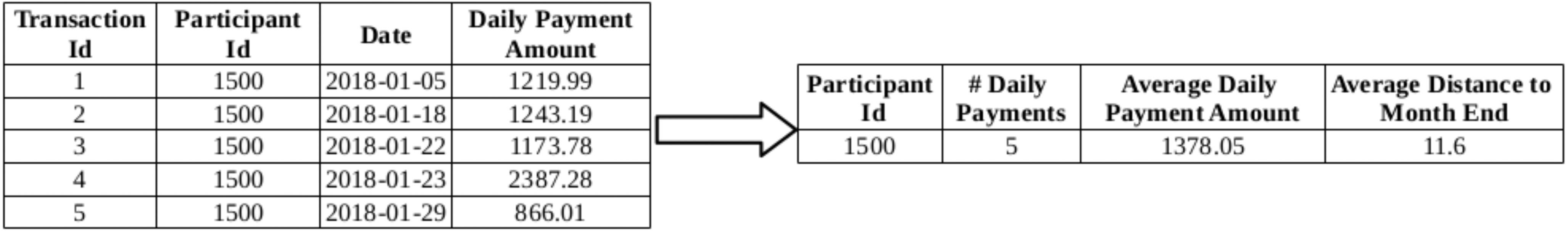
The most common approach for extracting features from the recurring data is to use statistical features like the average and count of the features belonging to each entity. From the daily payment transactions data, the number of transactions, average monetary amount of those transactions and the average age (in terms of days) of the transactions are extracted (see Fig. 1). For example, for the participant with Id 1500, the distance of each transaction to the end of the current month is 26, 13, 9, 8 and 2; so the average distance to the end of the month (2018-01-31) is found as 11.6 days. Similarly, these three features have been extracted for the daily penalty, monthly payment and monthly penalty transactions of each participant. This way, each participant will be described by 12 features (3 features
Figure 2.
RFM features extracted from the daily payment transactions for a single participant.
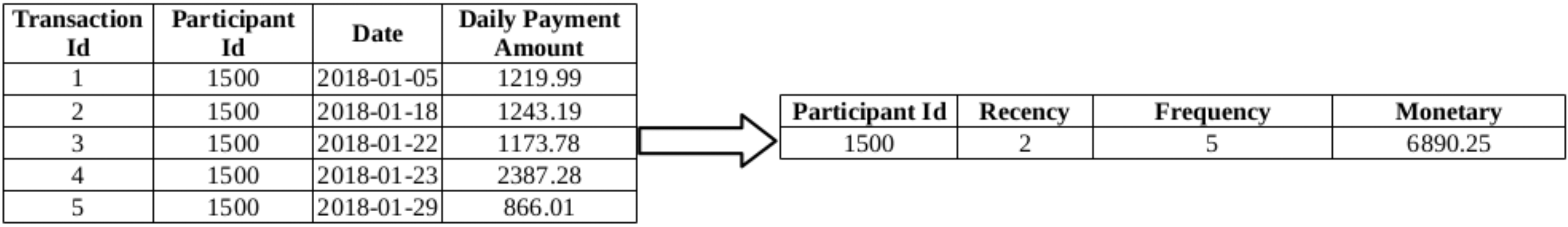
Figure 3.
RFM values and corresponding RFM scores of some participants.
3.1.2Preprocessing with RFM scoring
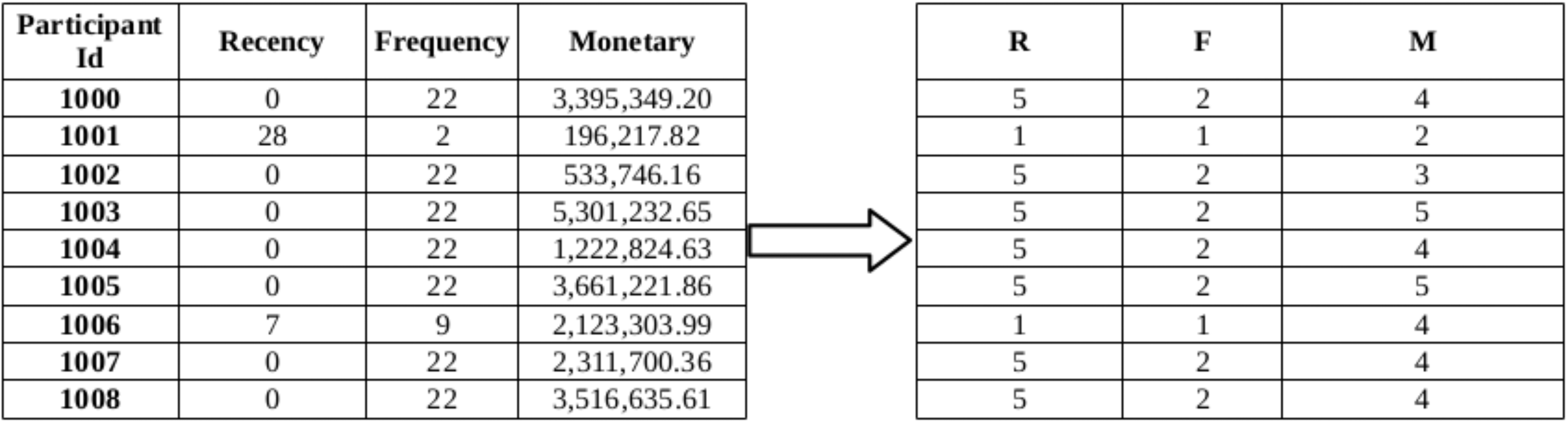
The RFM scoring approach requires extraction of the three features namely, Recency (R), Frequency (F) and Monetary (M) features. For a given participant, R represents the days since the last transaction, F represents the number of transactions, and M represents the total monetary values of the transactions. In RFM analysis, the participants are first segmented according to their R values. They are put in increasing order of their R values, and are splitted into 5 equal-sized groups, each group having a code ranging from 5 to 1, where 5 represents the customer group with the most recent transactions while 1 represents the customer group with the least recent transactions. The same process is repeated for F attribute and then for M attribute. Then, these coded RFM attributes for each customer are concatenated yielding a code that ranges from ‘555’ to ‘111’, where ‘555’ represents the most desired customer segment with respect to all three criteria, and ‘111’ represents the weakest customer segment. For example, in 2, first Recency, Frequency and Monetary values are calculated for the participant. After these values are computed for all of the participants, these values are converted into RFM scores ranging from 1 to 5 as shown in Fig. 3.
The RFM attributes for the daily cash clearing transaction dataset can be interpreted as follows: F is the number of transactions that a participant has made in a month, R represents the time interval between a participant’s last transaction date and the last transaction date in the monthly dataset, and M represents the total amount of debt paid on time (without penalty). The participants making recent, frequent transactions and paying huge debts on time are among the most desired participants; therefore they are given a score of ‘5’ for e refers to the value of the best group according to that attribute. In addition to the RFM scores extracted from the daily payment transactions dataset, three more RFM scores are extracted from each of the daily penalty, monthly payment and monthly penalty transactions datasets, as well. Each participant is again described by 12 features (3 for RFM
3.1.3Handling missing values
There are some participants with many records in the daily penalty dataset, but with no records in the daily payments dataset. No RFM scores regarding daily payments are generated for these participants. In order to get a complete picture of the payment behaviors of the participants, these missing values should be filled in properly. In the case where the raw data is used for creating clusters of participants, these missing values can all be replaced with ‘0’, safely. However, for the RFM attributes, the missing values should be handled properly. For the daily and monthly payments transactions dataset, each missing RFM attribute value is replaced with a ‘1’; for the daily and monthly penalty transactions datasets, each missing RFM attribute value is replaced with a ‘5’ because the participants with no incurring penalties are among the most desired participants. It is also important to note that some participants happen to be in the monthly transactions dataset but do not happen to be in the daily transactions dataset. These participants in the Balancing Power Market are directly managed by the EXIST and their financial status can only be seen after EXIST issues an invoice for them at the end of the month. Among 891 distinct participants that perform any kind of transactions in January 2018, 112 of them take place in Balancing Power Market only. The missing values regarding daily payment and penalty transactions for these participants are replaced with the best score of ‘5’.
After all the preprocessing steps, three datasets that includes features extracted from 4 different transaction types are as follows:
1. Mean values dataset: Average age of the transactions, total number of transactions, and average monetary value of the transactions are kept for each participant.
2. RFM values dataset: Age of the latest transaction, total number of transactions and the total monetary value of the transactions are kept for each participant.
3. RFM scores dataset: RFM Values dataset records are replaced with corresponding RFM Scores.
3.2Clustering algorithms
3.2.1K-means
K-means and its variants are among the most heavily-used clustering techniques for customer segmentation (see [19]). In its simplest form, K-means starts by selecting
3.2.2DBSCAN
DBSCAN algorithm can find clusters of any shape, as opposed to K-means algorithm which assumes that the clusters are convex-shaped. Clusters are formed as areas of high density seperated by areas of low density. The samples that are in areas of high density are called core samples and a set of these core samples form a cluster. A cluster consists of a set of core samples and a set of non-core samples that are close to a core sample. The term high density is defined by two parameters of the algorithm: min_points and eps. A core sample is a sample in the dataset such that there exist at least min_points number of other samples within a distance of eps. These samples are defined as neighbors of the core sample. A cluster can be built by recursively taking a core sample, finding all of its neighbors that are core samples, and finding all of the neighbors of that core samples, and so on (for the implementation details see [15]). Non-core samples that are neighbors of a core sample take place in the same cluster.
The parameter min_points controls the algorthm’s tolerance towards noice and is set to large values on noisy and large data sets. The parameter eps controls the local neighborhood of the points and should be selected carefully, because if it is selected too large, then all the samples can be put ito one cluster, or if it is selected too small, each sample can be clustered in its own cluster. Sander et al. [16] suggests setting min_points to twice the dataset dimensionality, and increasing its value for noisy and high-dimensional datasets.
Figure 4.
Elbow method illustration using SSE and silhouette score metrics.
3.2.3Agglomerative Clustering
Agglomerative Clustering belongs to the class of hierarchical clustering algorithms which create a hierarchical decomposition of the given data objects either agglomerative or divisive, depending on whether the hierarchical decomposition is formed in a bottom-up (merging) or top-down (splitting) fashion. The bottom-up approach, also called the agglomerative approach, starts by letting each object forming its own cluster and it successively merges the objects close to one another forming larger clusters with respect to a linkage criterion, until all the clusters are merged into one, or a termination condition holds (see [13]). The linkage criterion determines how to measure the distance between the pairs of clusters, then the algorithm merges the pairs of clusters that minimize this criterion. The linkage criterion can be one of the followings: ward, complete, average and single. ward uses the variance, whereas average uses the average of the distances of the points in the two clusters that is to be merged. complete or maximum linkage uses the maximum distances between all points of the two clusters, and single uses the minimum of the distances between all points of the two clusters.
3.2.4Measuring clustering quality
Extrinsic methods are used to evaluate the quality of the clusters, if the ground truth is available. However, in our case, intrinsic methods have been used due to the unavailability of the ground truth. Sum-of-Squared-Error and the Silhouette coefficient are among the most widely used intrinsic methods. Sum-of-Squared-Error (SSE) measure defines the homogeneity of the clustering results by summing over the squared distances between the clustering objects and their cluster centers for each cluster. SSE of a clustering
The silhouette coefficient method [13] evaluates the clustering results by assessing the separation and the compactness of the clusters. In order to compute the silhouette coefficient for a given clustering with
3.2.5Determining optimal number of clusters
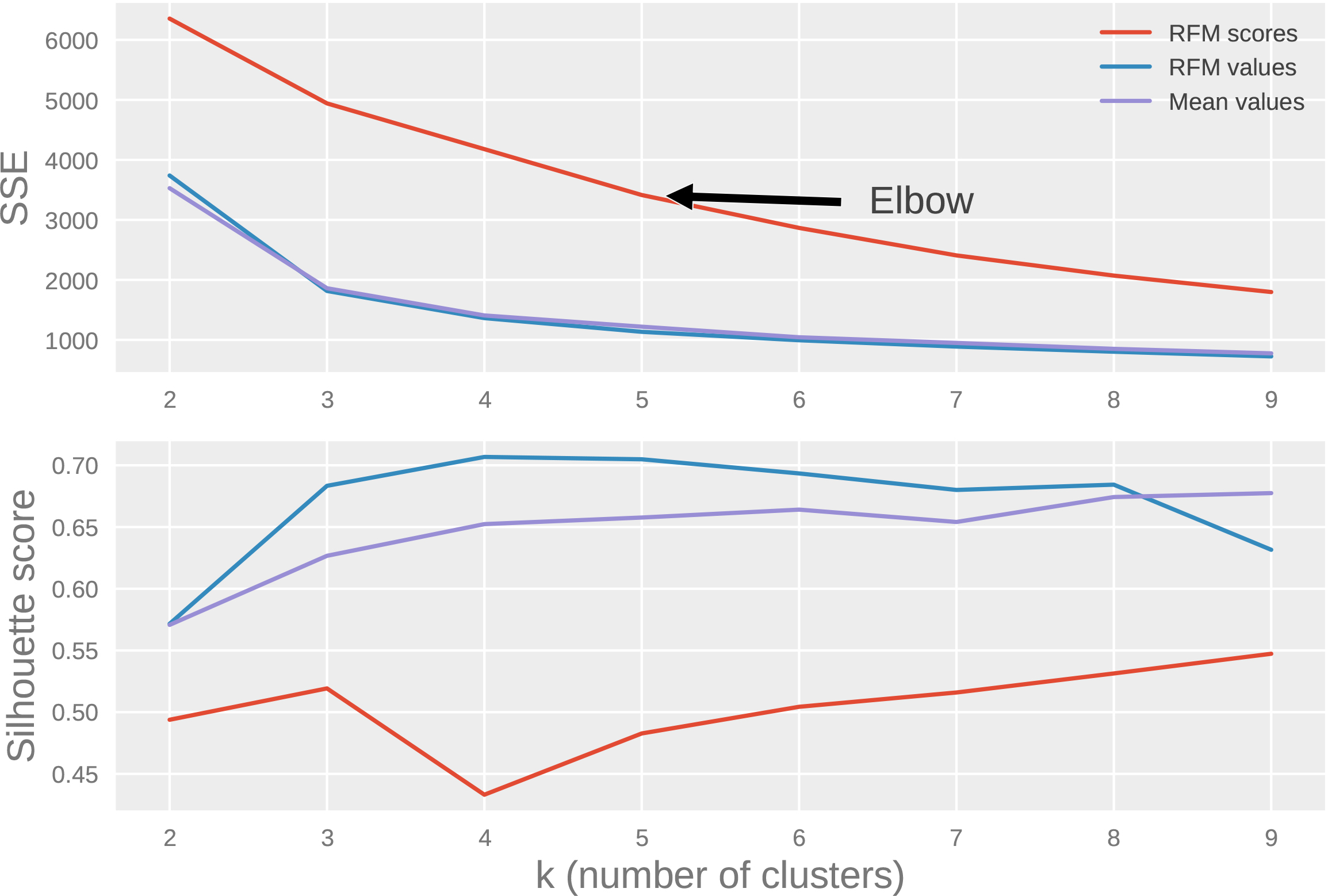
The Elbow method is based on the observation that increasing number of clusters reduces SSE. However, the marginal effect of reducing SSE may drop if too many clusters are formed. In the elbow method, the curve plot of SSE with respect to each selected number of clusters,
Figure 4 illustrates the elbow method using SSE metric and silhouette coefficient for each of the three datasets. One can see from the figure that the rate of reduction in SSE drops after 5; therefore 5 seems to be a good value for
Figure 5.
Elbow method illustration using SSE and silhouette score metrics for RFM values dataset.
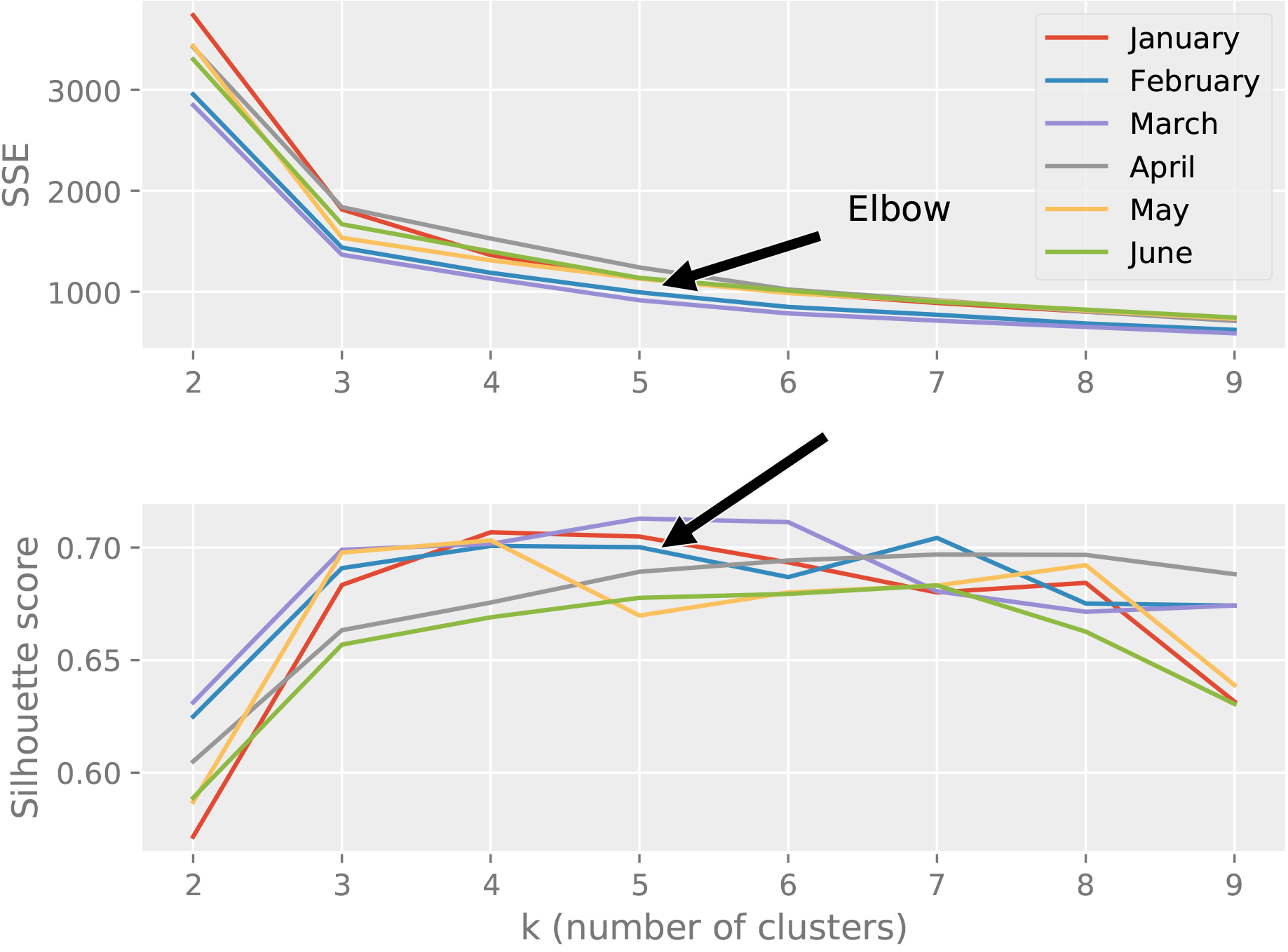
Figure 6.
Silhouette analysis – RFM values.
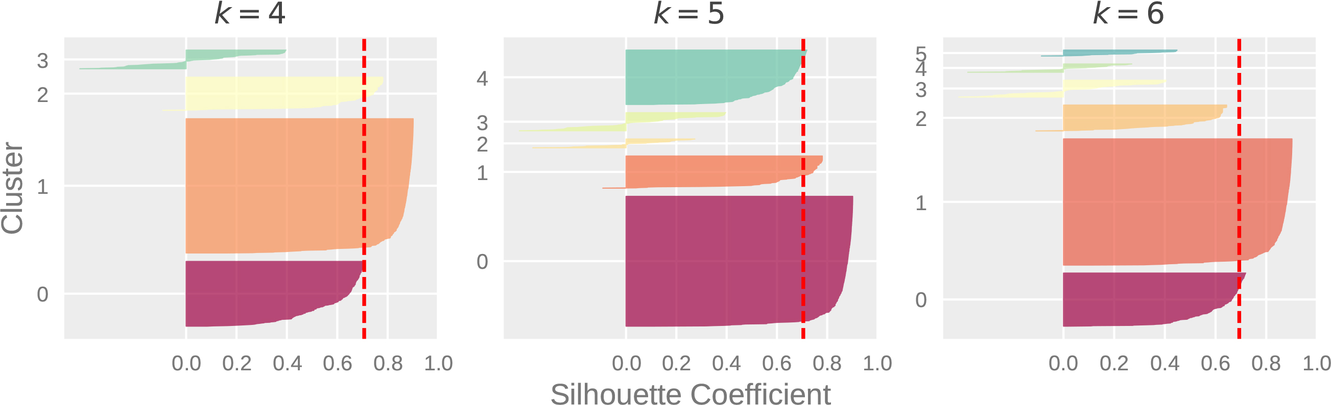
Silhoutte Analysis can also be used to check the decision on
4.Results
K-means is initialized multiple times with different centroid seeds, and the best output of in terms of SSE is selected. For the DBSCAN algorithm, we tested the values in {12, 24, 36, 48} and {0.5, 1, 1.5, 2, 2.5, 3} for min_points and eps parameters, respectively, and selected the values that gives the highest silhouette score. Forthe RFM scores dataset min_points
Table 3
Mean attribute values of the RFM scores dataset clusters formed with Agglomerative Clustering
| Daily payment | Daily penalty | Monthly payment | Monthly penalty | |||||||||
|---|---|---|---|---|---|---|---|---|---|---|---|---|
| Cluster | R | F | M | R | F | M | R | F | M | R | F | M |
| C1 | 4.66 | 2.19 | 3.25 | 4.90 | 4.93 | 4.90 | 4.47 | 3.44 | 4.17 | 5.00 | 5.00 | 5.00 |
| C2 | 5.00 | 5.00 | 5.00 | 5.00 | 5.00 | 5.00 | 1.00 | 1.00 | 1.00 | 2.33 | 3.67 | 4.00 |
| C3 | 1.00 | 1.00 | 1.00 | 1.00 | 2.00 | 5.00 | 5.00 | 1.00 | 3.00 | 1.00 | 5.00 | 2.00 |
| C4 | 1.00 | 1.00 | 1.00 | 5.00 | 3.00 | 4.00 | 1.00 | 1.00 | 1.00 | 1.00 | 1.00 | 1.00 |
| C5 | 1.00 | 1.00 | 1.00 | 1.00 | 1.00 | 2.00 | 1.00 | 1.00 | 1.00 | 1.00 | 5.00 | 1.00 |
| Mean: | 2.53 | 2.04 | 2.25 | 3.38 | 3.19 | 4.18 | 2.49 | 1.49 | 2.03 | 2.07 | 3.93 | 2.60 |
Figure 7.
Comparison of the algorithms w.r.t. silhouette scores computed using a) euclidean distance, b) cosine distance.
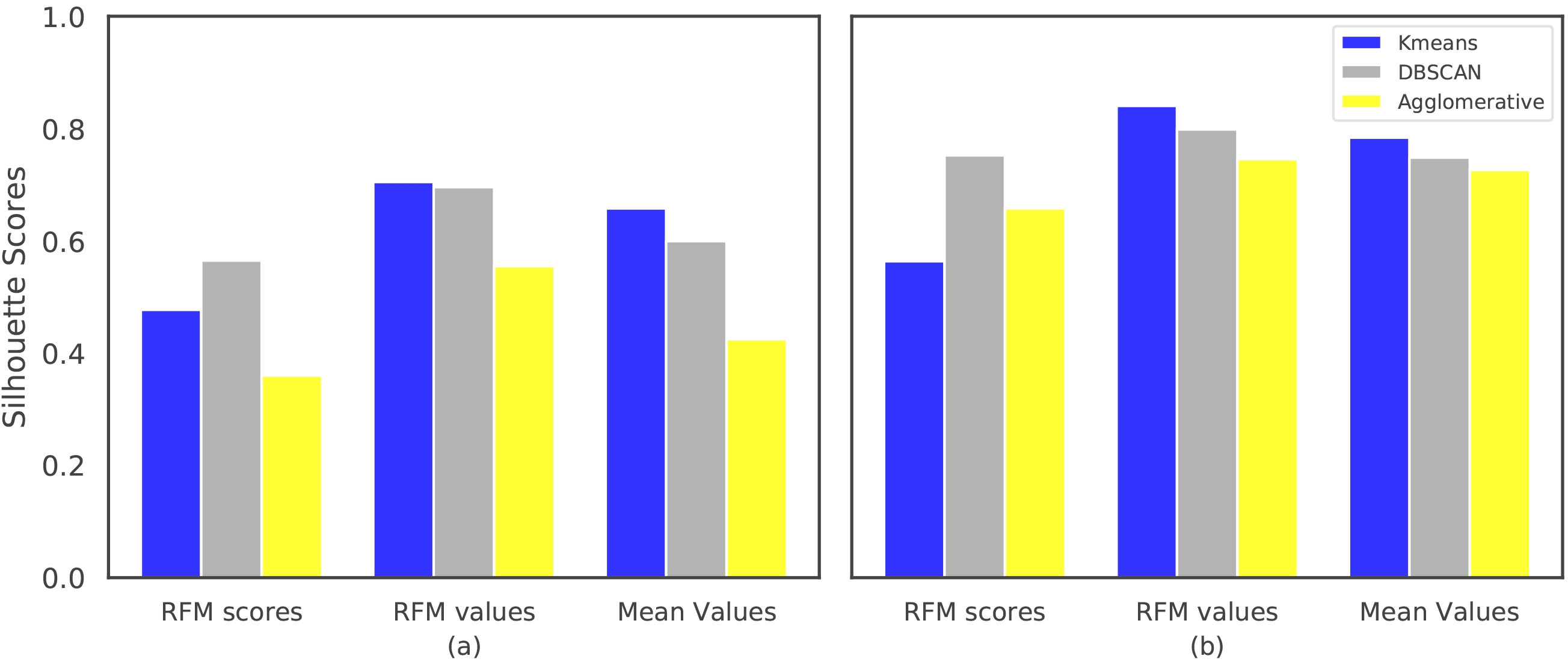
Figure 8.
Silhouette scores with cosine distance metric on non-normalized RFM values and mean values datasets.
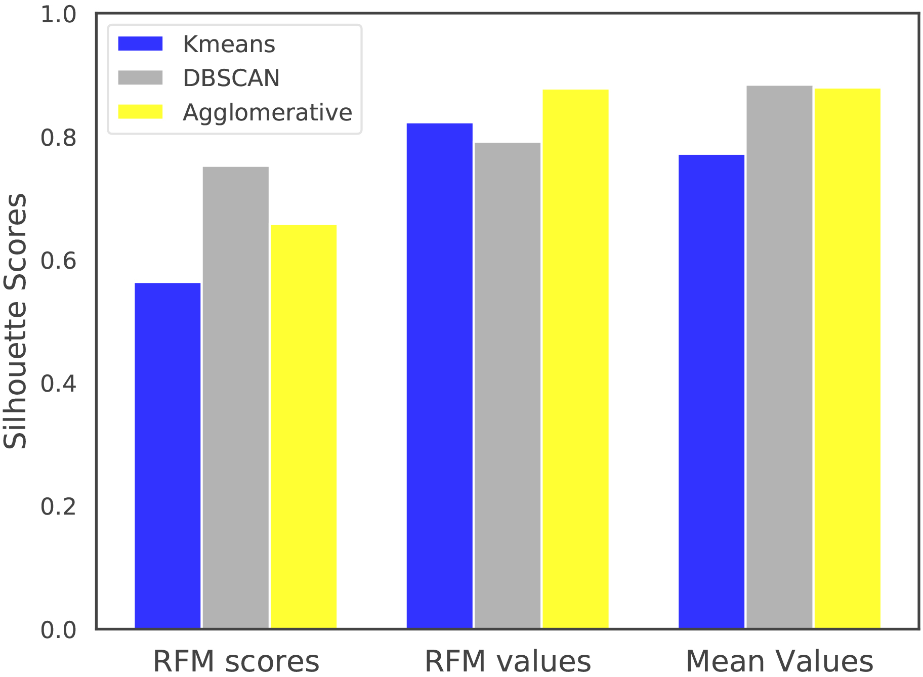
Table 4
Kmeans and Agglomerative Clustering statistics for RFM scores dataset
| Kmeans | Agglomerative | |||
|---|---|---|---|---|
| Cluster | Size | Colmns | Size | Colmns |
| C1 | 193 | 0.83 | 885 | 1.00 |
| C2 | 212 | 0.42 | 3 | 0.67 |
| C3 | 112 | 0.58 | 1 | 0.33 |
| C4 | 296 | 0.92 | 1 | 0.08 |
| C5 | 78 | 0.25 | 1 | 0.08 |
Firstly, the quality of the clusterings for the normalized datasets are compared in terms of the average Silhouette scores computed with Euclidean distance. Secondly, the clusterings have been compared using Cosine distance, as DBSCAN and Agglomerative Clustering algorithms allow using this distance metric. For DBSCAN eps parameter, the values in {0.01, 0.05, 0.1} have been evaluated and (min_points and eps) parameters are selected as (48, 0.1), (12, 0.01) and (12, 0.1) for RFM scores, RFM values and Mean values datasets, respectively. The results given in Fig. 7a suggest that Kmeans achieves better clusterings than DBSCAN for the RFM values and Mean values datasets according to the silhouette scores computed using euclidean distance. When cosine distance is used for forming and the evaluating the clusters, one can see from the results in Fig. 7b that Agglomerative Clustering is now able to generate competitive results with Kmeans and DBSCAN. Although Kmeans clusters are formed using euclidean distance, it still performs well with respect to the silhouette scores computed using cosine distance. It is also important to note that, the results shown in Fig. 7 are obtained using the normalized versions of RFM values and Mean values datasets. When non-normalized versions of these datasets are used in the clustering algorithms with cosine distance (except Kmeans), the results in Fig. 8 suggest that Agglomerative Clustering yields very well-seperated and compact clusters.
Table 5
Mean attribute values of the RFM values dataset clusters formed with Agglomerative Clustering
| Daily payment | Daily penalty | Monthly payment | Monthly penalty | ||||||||||
|---|---|---|---|---|---|---|---|---|---|---|---|---|---|
| Cluster | Size | R | F | M | R | F | M | R | F | M | R | F | M |
| C1 | 732 | 0.03 | 20.77 | 5.88 | 0.57 | 0.19 | 0.08 | 2.58 | 0.33 | 1.75 | 0.03 | 0.00 | 0.00 |
| C2 | 3 | 8.33 | 0.00 | 0.00 | 0.00 | 0.00 | 0.00 | 0.00 | 0.00 | 0.00 | 8.33 | 6.00 | 0.23 |
| C3 | 113 | 0.00 | 0.12 | 0.16 | 0.00 | 0.00 | 0.00 | 8.81 | 1.06 | 3.41 | 0.00 | 0.00 | 0.00 |
| C4 | 2 | 3.50 | 4.00 | 2.49 | 25.00 | 1.50 | 0.57 | 0.00 | 0.00 | 0.00 | 3.50 | 1.00 | 1.17 |
| C5 | 41 | 0.00 | 3.00 | 4.37 | 0.00 | 0.00 | 0.00 | 4.02 | 0.49 | 2.06 | 0.00 | 0.00 | 0.00 |
| Average | 2.37 | 5.58 | 2.58 | 5.11 | 0.34 | 0.13 | 3.08 | 0.38 | 1.44 | 2.37 | 1.40 | 0.28 | |
In order to perform a better comparison among the clustering algorithms, we also utilize the clustering statistics. For illustration purposes, we consider the clusters formed by Kmeans and Agglomerative Clustering algorithms for the the RFM scores dataset (transactions regarding January 2018). In RFM analysis, RFM pattern of each participant/customer is extracted by comparing the cluster’s average with the overall average for each attribute (see Table 3 for Agglomerative Clustering statistics). For a given attribute A, if the cluster average is less than the overall average, then ‘A
We also compare the algorithms using the clustering statistics for RFM values dataset due to high silhoutte scores (see Figs 7 and 8). High silhoutte scores suggest that RFM values dataset clusterings can help identify high-risk participants better than the other datasets. But this should also be confirmed by evaluating the clustering statistics, as well.
Table 6
Number of participants in each segment
| Month | Very high-risk | High-risk | Medium-risk | Low-risk | Very low-risk | Total |
|---|---|---|---|---|---|---|
| January | 2 | 3 | 0 | 154 | 732 | 891 |
| February | 5 | 3 | 15 | 120 | 751 | 894 |
| March | 0 | 4 | 13 | 145 | 753 | 915 |
| April | 0 | 0 | 27 | 123 | 766 | 916 |
| May | 3 | 0 | 27 | 116 | 774 | 920 |
| June | 5 | 0 | 126 | 17 | 771 | 919 |
The clusterings formed by Agglomerative Clustering using RFM values dataset are used to assign the participants to the following risk segments: very high-risk segment, high-risk segment, medium-risk segment, low-risk segment and very low-risk segment. The characteristics of the participants for each segment can be summarized as follows:
1. Very low-risk segment represents the participants with frequent daily and monthly payments with very large amounts and very little or no penalties.
2. Low-risk segment represents the participants whose payment behaviors are similar to that of very low-risk segment participants, but the payment frequency and the amounts are not as large as those payments.
3. Medium-risk segment represents the participants with little penalties, infrequent daily and monthly payments with small or even zero amounts. The participants with frequent daily payments with large amounts, but with large daily or monthly penalties also take place in this segment, because these participants should be monitored closely.
4. High-risk segment represents the participants with infrequent daily or monthly payments with small or zero amounts, large monthly penalties.
5. Very high-risk segment represents the participants with infrequent daily or monthly payments with very small or zero amounts, very large monthly penalties.
When we analyze the clusterings for non-normalized RFM values dataset with the help of domain expert, we realize that applying a simple log transformation on monetary values result in better separated clusters than applying no transformation at all. One can see from Table 5 that the clusters are well-separated according to all of the attributes. It can easily be distinguished from the table that C1 and C3 represents very low-risk and low-risk participants, respectively with high daily and monthly payments and low daily and monthly penalties. C5 can also be considered as low-risk group due to large daily and monthly payments and zero penalties. It is clear from the table that C4 represents very-high risk participants, while C2 represents high risk participants. The number of participants for each segment for the first 6 months data, is shown in Table 6.
It is also important to note that setting the number of clusters as “five” does not mean that five risk segments will be created. For example, five clusters have been created (see Tables 5 and 6), but after carefully assessing the cluster statistics, some of these clusters are merged into a single cluster representing a single risk segment. When the number of participants in each risk segment is carefully analyzed, one can see from Table 6 that there is a slight deviation in the pattern of the number of medium-risk participants in June. This is explained by the economic conditions due to surge in foreign currency.
5.Conclusion
In this study, segments of Electricity Market participants have been created by taking into account the transactions arising from all market activities with the aim of identifying high-risk participants. This segmentation information is then used for fairly valuing the collaterals for the market participants. Using the debt payment transactions dataset provided by the central settlement bank, we have created different representations of the data and compared these approaches in terms of representing the payment behaviors of the participants well. In order to create clusterings for each of these datasets, three clustering algorithms, namely, K-means, DBSCAN and Agglomerative Clustering are employed. Silhouette score metric is used for comparing different clustering algorithms on different representations of the data. It is clear from the results that the quality of the clusterings are greatly affected by the clustering distance metric. Moreover, the selection of the representation for the data is crucial for well-separation of the clusters. The RFM scoring technique did not provide expected results; but using the actual (non-normalized) RFM values in Agglomerative Clustering with cosine distance yielded in very well-seperated and compact clusters. The participants belong to high-risk or very high-risk segment are clearly distinguishable. It is also acknowledged by the domain expert that the results are as expected.
This study can be extended by considering the debt payment transactions of the participants other than immediately preceding month. This way, the participants that take place in the risky segment as the first time can be distinguished from the participants that take place in the risky segment frequently.
References
[1] | Hughes AM. Strategic database marketing, Chicago, IL: Probus Publishing, (1994) . |
[2] | Hsieh NC. An integrated data mining and behavioral scoring model for analyzing bank customers, Expert systems with applications, 27: (4), (2004) , 623–633. |
[3] | Lumsden SA, Beldona S, Morrison AM. Customer value in an all-inclusive travel vacation club: an application of the RFM framework, Journal of Hospitality & Leisure Marketing, 16: (3), (2008) , 270–285. |
[4] | Liu DR, Shih YY. Hybrid approaches to product recommendation based on customer lifetime value and purchase preferences, J. Syst. Softw., 77: (2), (2005) , 181–191. |
[5] | Chang H, Tsai H. Group RFM analysis as a novel framework to discover better customer consumption behavior, Expert Syst. Appl., 38: (12), (2011) , 14499–14513. |
[6] | Birant D. Data Mining Using RFM Analysis, Knowledge-Oriented Applications in Data Mining, INTECH Open Access Publisher, (2011) . |
[7] | Wu H, Chang E, Lo C. Applying RFM model and K-means method in customer value analysis of an outfitter, International Conference on Concurrent Engineering, New York, (2009) . |
[8] | Namvar M, Gholamian MR, KhakAbi S. A two phase clustering method for intelligent customer segmentation, International Conference on Intelligent Systems, Modelling and Simulation, IEEE, (2010) . |
[9] | Mo JY, Kiang M, Zou P, Li P. A two-stage clustering approach for multi-region segmentation, Expert Syst. Appl., 37: (10), (2010) , 7120–7131. |
[10] | Aggelis V, Christodoulakis ND. Customer clustering using RFM analysis, Computer Engineering and Informatics Department University of Patras, Patras, GREECE, (2005) . |
[11] | Naik C, Kharwar A, Desai N. A review: RFM approach on different data mining techniques, International Journal of Emerging Technology and Advanced Engineering, Journal, 3: (Issue 10), (2013) . |
[12] | Elmas Ö. Mü şteri Analiti ği ve Öneri Sistemleri Uygulaması, Yayınlanmışs Yüksek Lisans Tezi, Istanbul Teknik Üniversitesi, Fen Bilimleri Enstitüsü, Istanbul, (2018) . |
[13] | Kaufman L, Rousseeuw PJ. Finding Groups in Data: An Introduction to Cluster Analysis, John Wiley & Sons, (1990) . |
[14] | Arthur D, Vassilvitskii S. K-means++: The advantages of careful seeding, In Proceedings of the eighteenth annual ACM-SIAM symposium on Discrete algorithms, Society for Industrial and Applied Mathematics, (2007) . |
[15] | Schubert E, Sander J, Ester M, Kriegel HP, Xu X. DBSCAN revisited, revisited: why and how you should (still) use DBSCAN, ACM Transactions on Database Systems (TODS), 42: (3), (2017) , 19. |
[16] | Sander J, Ester M, Kriegel HP, et al. Data Mining and Knowledge Discovery 2: (1998) , 169. |
[17] | Liu F, Zhao S, Li Y. How many, how often, and how new? A multivariate profiling of mobile app users, Journal of Retailing and Consumer Services, 38: , (2017) , 71–80. |
[18] | Chen D, Sain SL, Guo K. Data mining for the online retail industry: a case study of RFM model-based customer segmentation using data mining, Journal of Database Marketing & Customer Strategy Management, 19: (3), (2012) , 197–208. |
[19] | Khalili-Damghani K, Abdi F, Abolmakarem S. Hybrid soft computing approach based on clustering, rule mining, and decision tree analysis for customer segmentation problem: real case of customer-centric industries, Applied Soft Computing, 73: , (2018) , 816–828. |
[20] | Stormi K, Lindholm A, Laine T, Korhonen T. RFM customer analysis for product-oriented services and service business development: an interventionist case study of two machinery manufacturers, Journal of Management and Governance, (2019) , 1–31. |
[21] | Han J, Pei J, Kamber M. Data mining: concepts and techniques, Elsevier, (2011) . |

