
Comparative analysis of evolutionary algorithms for multiple criteria decision making with interval-valued belief distributions
Abstract
In multiple criteria decision making (MCDM) with interval-valued belief distributions (IVBDs), individual IVBDs on multiple criteria are combined explicitly or implicitly to generate the expected utilities of alternatives, which can be used to make decisions with the aid of decision rules. To analyze an MCDM problem with a large number of criteria and grades used to profile IVBDs, effective algorithms are required to find the solutions to the optimization models within a large feasible region. An important issue is to identify an algorithm suitable for finding accurate solutions within a limited or acceptable time. To address this issue, four representative evolutionary algorithms, including genetic algorithm, differential evolution algorithm, particle swarm optimization algorithm, and gravitational search algorithm, are selected to combine individual IVBDs of alternatives and generate the minimum and maximum expected utilities of alternatives. By performing experiments with different numbers of criteria and grades, a comparative analysis of the four algorithms is provided with the aid of two indicators: accuracy and efficiency. Experimental results indicate that particle swarm optimization algorithm is the best among the four algorithms for combining individual IVBDs and generating the minimum and maximum expected utilities of alternatives.
1.Introduction
In the Internet and Big Data era, human lifestyles have undergone an unprecedented revolution. An individual’s life is filled with a lot of data, which makes people more informed than ever before. At the same time, people must choose between deriving useful information and knowledge from data for use in practice and abandoning their attempt to employ data in real problems. Because of the availability of information, people usually choose to find effective information and knowledge from various types of data and use them in practical cases. Such a choice improves their capability to handle complex problems. The choice also results in more uncertain environments associated with real problems than before due to the randomness, unavailability, noise, sparsity, and variety of data. In this environment, people may have difficulty directly finding overall solutions to real problems. A feasible way to overcome the difficulty is to analyze real problems from multiple different perspectives, and then combine the relevant analyses to generate overall problem solutions. This method is called multiple criteria decision making (MCDM) in an uncertain environment.
To effectively model and analyze uncertain MCDM problems, many attempts have been made with the help of different uncertain expressions. Representative expressions include intuitionistic fuzzy sets [1], hesitant fuzzy linguistic sets [2], hesitant fuzzy sets [3], probabilistic linguistic sets [4], belief distributions [5], interval-valued fuzzy sets [6], interval-valued hesitant fuzzy linguistic sets [7], interval-valued intuitionistic fuzzy sets [8], interval-valued hesitant fuzzy sets [9], interval type-2 fuzzy sets [10], and interval-valued belief distributions [11]. In theory, MCDM methods with these expressions are sufficient for analyzing all real problems. From real cases or numerical examples in these studies, few methods are found which aim to solve large-scale problems with many alternatives and criteria. In addition to this, when interval-valued assessments are adopted, such as interval-valued hesitant fuzzy elements or interval-valued belief distributions, the search space for finding solutions increases exponentially with the increase in the number of interval-valued hesitant fuzzy element values or the number of interval-valued belief distribution grades.
Evolutionary computation provides a feasible and effective way to find acceptable or satisfactory solutions within a limited time. When MCDM problems are regarded as multi-objective optimization (MOO) problems constructed on a common set of variables, many evolutionary MOO approaches have been developed to find the optimum trade-off among criteria which is the most consistent with the preference of a decision maker [12, 13, 14, 15, 16, 17]. Three methods (priori, interactive, and posteriori) are usually applied to combine the preferences of a decision maker with the MOO process [15, 16]. If the preferences of a decision maker are not considered in the MOO process, the results of the MOO may not be satisfactory.
In practice, individual assessments on different criteria may not be always constructed on a common set of variables. For example, a radiologist determines whether a nodule of a patient is malignant from the perspectives of contour, echogenicity, calcification, and vascularity. It cannot be said that the judgments on the nodule with the consideration of contour and those with the consideration of any other perspective are made by the radiologist through the same set of variables (or features). As another example, when the same discipline at different universities is compared, many criteria are considered, such as research projects, publications, awards, patents, social services, and excellent alumni. Individual assessments on different criteria are generated from different data rather than common data. When encountering these situations, a decision maker takes into account the individual assessments on all criteria synthetically rather than improving the values of most objectives and balancing them to generate solutions. MCDM problems with large search spaces in these situations can also be solved by using evolutionary algorithms. For example, Javanbarg et al. [18] used particle swarm optimization (PSO) algorithm [19] to solve MCDM problems modeled by a fuzzy analytic hierarchy process, and Chen and Huang [20] used PSO algorithm to solve MCDM problems modeled by interval-valued intuitionistic fuzzy numbers.
Existing studies show that less attention has been paid to the application of evolutionary algorithms to MCDM with different sets of variables used on different criteria. This makes it questionable whether MCDM methods with different ways to characterize different types of uncertain nature (e.g., [3, 7, 8, 9, 10, 11]) can be applied to solve MCDM problems with large search spaces. There is a gap between the solution requirements of large-scale MCDM problems and relevant studies on effective solution approaches. Although there are few studies on the combination of evolutionary algorithms and MCDM with different sets of variables (e.g., [18, 20]), some important issues deserve investigation. The issues include: (1) why PSO algorithm has been selected for application in MCDM; (2) whether PSO algorithm can be applied to MCDM with different types of uncertain expressions other than interval-valued intuitionistic fuzzy numbers and fuzzy triangular numbers; and (3) which evolutionary algorithm has better performance when applied to MCDM with a specific type of uncertain expression. In fact, different evolutionary algorithms can be applied to solve the same real problem. For example, when determining the near-optimal scheme for recharging batteries at a battery swapping station, Wu et al. [21] used three representative evolutionary algorithms including genetic algorithm (GA) [22, 23], differential evolution (DE) algorithm [24], and PSO algorithm to find the minimum running cost. Their experimental results show that GA and DE algorithms achieve higher accuracies and lower efficiencies than PSO algorithm; specifically, PSO algorithm fails to obtain the objective. Inspired by this, much attention should be paid to a key issue, which is comparing the accuracies [21, 25] and efficiencies [14, 26] of different representative evolutionary algorithms for solving large-scale MCDM problems with specific types of uncertain expressions and different sets of variables.
In this paper, to address this key issue, we aim to compare the accuracies and efficiencies of four representative evolutionary algorithms, which are GA, DE algorithm, PSO algorithm, and gravitational search algorithm (GSA) [27], for analyzing MCDM problems modeled by interval-valued belief distributions (see Section 2). Because combining individual interval-valued belief distributions is an important and necessary MCDM sub-process of MCDM, the combination processes using the four algorithms are presented. To fairly compare the four algorithms, their original versions (instead of their extensions) are used in the processes. With the aid of the processes, experiments with different numbers of criteria and grades used to profile interval-valued belief distributions are performed to compare the accuracies and efficiencies of the four algorithms for combining interval-valued belief distributions and generating the expected utilities. The comparative analysis of experimental results helps select the appropriate evolutionary algorithm to find satisfactory solutions to MCDM problems with interval-valued belief distributions within a limited or acceptable time. A sensitivity analysis of the accuracies and efficiencies of the four algorithms is provided to highlight the conclusion drawn from the comparative analysis.
The rest of this paper is organized as follows. Section 2 recalls the modeling of MCDM problems by using belief distributions and interval-valued belief distributions. Section 3 presents the processes of four evolutionary algorithms for combining interval-valued belief distributions. Section 4 compares the accuracies and efficiencies of the four algorithms for combining interval-valued belief distributions. The results of the four algorithms for generating the expected utilities are compared in Section 5. A sensitivity analysis of the performance of the four algorithms is provided in Section 6. Finally, this paper is concluded in Section 7.
2.Preliminaries
2.1Modeling of MCDM problems using belief distributions
In the evidential reasoning (ER) approach [28, 29, 30], which is a type of multiple criteria utility function method, belief distribution is used to characterize the uncertain preferences of a decision maker. Because belief distribution is a special case of interval-valued belief distribution, the method for modeling MCDM problems using belief distribution is reviewed first.
Suppose that alternative
Assume that criteria weights are represented by
2.2Combination of belief distributions
The contents in the above section show that the ER rule [32] is the key to find solutions to MCDM problems modeled by belief distributions, which is simply presented as follows.
.
[32] Given individual assessments
(1)
where
(2)
(3)
(4)
(5)
(6)
(7)
(8)
and
(9)
In Definition 1,
2.3Modeling of MCDM problems using interval- valued belief distributions
Due to the lack of sufficient data and knowledge or the nature of the decision problems under consideration, in some situations, a decision maker can only provide interval-valued belief distributions (IVBDs) as the evaluations of alternatives. For example, when a radiologist provides the diagnostic category in thyroid imaging reporting and data system published by Horvath et al. [34] for the thyroid nodule of a patient, he or she only reports the interval-valued cancer risk rather than the precise cancer risk of the patient.
In this situation, individual IVBDs are represented by
(10)
(11)
(12)
(13)
Normalized IVBDs are valid but valid IVBDs may be unnormalized [35].
From normalized individual IVBDs, a pair of optimization problems is constructed by using the ER rule to generate the aggregated IVBD
(14)
(15)
(16)
(17)
In the pair of optimization problems,
(18)
(21)
Solving this model, in which
(22)
(25)
The combination of individual belief distributions by using the ER rule to generate the aggregated belief distribution
3.Four evolutionary algorithms for MCDM with IVBDs
When the number of criteria
In the following, the original processes of the four evolutionary algorithms for solving the pair of optimization problems shown in Eqs (14)–(17) are presented to facilitate comparing the accuracies and efficiencies of the four algorithms. When the objective in Eq. (14) is changed to that in Eq. (22), the similar processes of the four algorithms can be used to determine the minimum and maximum expected utilities, which are omitted to avoid repetition. To guarantee a fair comparison, extensions of the four algorithms are not adopted.
3.1GA process for combining individual IVBDs
The GA process for combining individual IVBDs is presented as follows.
Step 1: Initialization
For the pair of optimization problems in Eqs (14)–(17), the
(26)
Randomly generating
Step 2: Performance evaluation
When the lower bound of
Step 3: Selection
The selection probability of the chromosome
(27)
where
Step 4: Crossover
After selection, two chromosomes
(28)
(29)
(30)
(31)
Step 5: Mutation
After the selection and crossover operations, a chromosome
(32)
(33)
where
(34)
(35)
As presented in Section 2.1,
(36)
and
(37)
When
(38)
(39)
where
(40)
and
(41)
By following a similar rule, the normalized belief distribution is obtained as
(42)
and
(43)
Note that as
Step 6: Update
After the selection, crossover, and mutation operations are performed, the fitness values of all chromosomes are recalculated to update the best objective with the corresponding solution.
Step 7: Termination
If
3.2DE algorithm process for combining individual IVBDs
The DE algorithm process for combining individual IVBDs is presented as follows.
Step 1: Initialization
For the pair of optimization problems in Eqs (14)–(17), the
(44)
The
Step 2: Performance evaluation
Through the same process as Section 3.1, the fitness value of the individual
Step 3: Mutation
For the individual
and
(46)
To guarantee that the mutated belief distribution is feasible,
Step 4: Crossover
Given a random indicator of crossover
(47)
and
(48)
Then, the crossed individual
Step 5: Selection
If the fitness value of the crossed individual
Step 6: Update
After the mutation, crossover, and selection operations are performed, the fitness values of all individuals are recalculated to update the best objective with the corresponding solution.
Step 7: Termination
If
3.3PSO algorithm process for combining individual IVBDs
The PSO algorithm process for combining individual IVBDs is presented as follows.
Step 1: Initialization
For the pair of optimization problems in Eqs (14)–(17), the position and the velocity of the
(49)
and
(50)
The
Step 2: Performance evaluation
Through the same process as Section 3.1, the fitness value of each particle is obtained. From the fitness values of all particles, the initial value of the best position of each particle and that of the best position of all particles are also obtained as
and
Step 3: Position update
Two random real numbers
(51)
and
(52)
To avoid extreme velocity,
From the updated velocity of the particle
(53)
(54)
To guarantee the feasibility of the updated position of the
The feasible updated position of the
Step 4: Best position update
After the positions of all particles are updated, the fitness values of all particles are recalculated to update the historical best position of each particle and the historical best position of all particles to be
Step 5: Termination
If
3.4GSA process for combining individual IVBDs
The GSA process for combining individual IVBDs is presented as follows.
Step 1: Initialization
For the pair of optimization problems in Eqs (14)–(17), the position and velocity of the
The
Step 2: Performance evaluation
Through the same process as Section 3.1, the fitness value of each agent is obtained.
Step 3: Update of gravitational coefficient and inertial mass
In the
(55)
and
(56)
respectively. By using
(57)
where
The passive and active gravitational masses
Step 4: Calculation of the total force acting on the j
In the
(58)
and
(59)
where
Assume that
(60)
(61)
where
Step 5: Calculation of acceleration and velocity
The acceleration of the
(62)
(63)
Step 6: Update of the agent’s position
From the acceleration of the
(64)
(65)
where
The resulting velocity is then used to calculate the updated position of the
(66)
(67)
Through the same process as Step 3 of Section 3.3, the normalized position of the
Step 7: Termination
If
4.Comparison for generating aggregated IVBDs
For a MCDM problem modeled by IVBDs, the aggregated IVBD of each alternative is usually used to analyze the problem. Although the final solution cannot be directly generated from the aggregated IVBDs of alternatives in most cases, beneficial analyses can be generally obtained. More importantly, the aggregated IVBDs of alternatives can be combined with the utilities of grades
Table 1
The optimal
| Parameters | GA | DE | PSO | GSA |
|---|---|---|---|---|
| (0.3, 10, 5) | (0.0782, 0.555) | (0.0625, 2.891) | (0.0376, 0.801) | (0.0662, 20.822) |
| (0.3, 14, 7) | (0.0512, 0.735) | (0.0415, 5.765) | (0.0328, 1.439) | (0.0594, 38.282) |
| (0.3, 18, 9) | (0.0590, 0.987) | (0.0320, 9.674) | (0.0270, 2.230) | (0.0473, 60.450) |
| (0.3, 22, 11) | (0.0291, 1.268) | (0.0262, 15.459) | (0.0224, 3.133) | (0.0482, 87.444) |
| (0.3, 26, 13) | (0.0374, 1.520) | (0.0217, 31.423) | (0.0193, 4.333) | (0.0339, 121.479) |
| (0.3, 30, 15) | (0.0400, 1.897) | (0.0184, 52.084) | (0.0175, 5.574) | (0.0405, 159.405) |
| (0.8, 10, 5) | (0.1431, 0.531) | (0.1327, 2.938) | (0.1287, 0.903) | (0.1308, 21.081) |
| (0.8, 14, 7) | (0.1067, 0.722) | (0.1008, 5.812) | (0.0979, 1.513) | (0.1051, 37.769) |
| (0.8, 18, 9) | (0.0822, 0.978) | (0.0796, 9.740) | (0.0786, 2.232) | (0.0842, 60.748) |
| (0.8, 22, 11) | (0.0733, 1.238) | (0.0666, 15.399) | (0.0657, 3.254) | (0.0730, 87.954) |
| (0.8, 26, 13) | (0.0631, 1.568) | (0.0569, 24.340) | (0.0565, 4.325) | (0.0629, 121.029) |
| (0.8, 30, 15) | (0.0546, 1.815) | (0.0497, 55.450) | (0.0495, 5.520) | (0.0529, 160.301) |
4.1Aggregation comparison of the four evolutionary algorithms by using specified IVBDs
Suppose that all individual IVBDs are normalized in a MCDM problem, which makes Eqs (2.3)–(2.3) hold. There are two types of situations in which IVBDs are normalized. One is that
and
or
and
while the other is that
The IVBDs in the first type of situation are regarded as specified and those in the second type of situation as general. In the following, specified IVBDs are first used as foundations to compare the accuracies [21] and efficiencies [14] of the four evolutionary algorithms presented in Section 3 for combining individual IVBDs.
We focus on the aggregation of specified IVBDs satisfying
and
For simplicity, assume that
with
and
With this assumption, without loss of generality, four evolutionary algorithms are used to determine
To fairly compare the four algorithms, it is specified that
Table 2
The optimal
| Parameters | GA | DE | PSO | GSA |
|---|---|---|---|---|
| (0.3, 10, 5) | (0.3850, 0.504) | (0.4790, 2.999) | (0.8115, 0.877) | (0.4714, 24.298) |
| (0.3, 14, 7) | (0.2941, 0.774) | (0.3896, 5.786) | (0.8018, 1.480) | (0.3740, 38.316) |
| (0.3, 18, 9) | (0.2166, 0.979) | (0.2923, 9.584) | (0.7204, 2.239) | (0.3326, 60.755) |
| (0.3, 22, 11) | (0.2081, 1.223) | (0.2789, 15.188) | (0.7305, 3.210) | (0.3090, 87.262) |
| (0.3, 26, 13) | (0.2098, 1.566) | (0.3248, 32.706) | (0.6827, 4.340) | (0.2828, 121.762) |
| (0.3, 30, 15) | (0.1593, 1.890) | (0.3135, 45.742) | (0.5694, 5.483) | (0.2701, 160.274) |
| (0.8, 10, 5) | (0.2181, 0.525) | (0.2451, 3.033) | (0.3564, 0.872) | (0.3062, 21.235) |
| (0.8, 14, 7) | (0.1621, 0.746) | (0.1805, 5.750) | (0.3052, 1.450) | (0.2447, 38.103) |
| (0.8, 18, 9) | (0.1404, 0.994) | (0.1591, 9.789) | (0.2752, 2.258) | (0.2009, 60.821) |
| (0.8, 22, 11) | (0.1123, 1.236) | (0.1416, 15.172) | (0.2555, 3.216) | (0.1790, 88.943) |
| (0.8, 26, 13) | (0.0982, 1.553) | (0.1308, 23.824) | (0.2504, 4.281) | (0.1661, 120.884) |
| (0.8, 30, 15) | (0.0907, 1.884) | (0.1305, 52.407) | (0.2388, 5.463) | (0.1570, 157.929) |
Suppose that the optimal values of
As for the optimal
Table 3
The optimal
| Parameters | GA | DE | PSO | GSA |
|---|---|---|---|---|
| (0.3, 10, 5) | (0.0701, 0.558) | (0.0700, 2.928) | (0.0678, 0.885) | (0.0701, 21.005) |
| (0.3, 14, 7) | (0.0536, 0.813) | (0.0536, 6.107) | (0.0531, 1.598) | (0.0537, 38.347) |
| (0.3, 18, 9) | (0.0434, 1.055) | (0.0434, 9.704) | (0.0434, 2.418) | (0.0434, 60.438) |
| (0.3, 22, 11) | (0.0364, 1.322) | (0.0364, 15.297) | (0.0364, 3.351) | (0.0364, 86.852) |
| (0.3, 26, 13) | (0.0313, 1.656) | (0.0313, 24.618) | (0.0313, 4.522) | (0.0313, 119.780) |
| (0.3, 30, 15) | (0.0275, 2.040) | (0.0275, 55.714) | (0.0275, 5.893) | (0.0275, 161.294) |
| (0.8, 10, 5) | (0.2016, 0.535) | (0.2016, 2.879) | (0.2007, 0.926) | (0.2015, 20.944) |
| (0.8, 14, 7) | (0.1510, 0.795) | (0.1509, 5.607) | (0.1505, 1.570) | (0.1509, 37.760) |
| (0.8, 18, 9) | (0.1206, 1.055) | (0.1206, 9.783) | (0.1206, 2.378) | (0.1206, 59.566) |
| (0.8, 22, 11) | (0.1004, 1.324) | (0.1004, 15.172) | (0.1004, 3.281) | (0.1005, 86.264) |
| (0.8, 26, 13) | (0.0860, 1.696) | (0.0860, 32.307) | (0.0860, 4.556) | (0.0860, 119.355) |
| (0.8, 30, 15) | (0.0753, 2.025) | (0.0753, 59.966) | (0.0753, 5.882) | (0.0753, 157.933) |
Table 4
The optimal
| Parameters | GA | DE | PSO | GSA |
|---|---|---|---|---|
| (0.3, 10, 5) | (0.1040, 0.554) | (0.3582, 2.907) | (0.465, 0.886) | (0.1003, 20.895) |
| (0.3, 14, 7) | (0.0668, 0.791) | (0.2703, 5.799) | (0.3426, 1.570) | (0.0701, 38.243) |
| (0.3, 18, 9) | (0.0603, 1.027) | (0.2177, 9.751) | (0.2711, 2.368) | (0.0532, 59.594) |
| (0.3, 22, 11) | (0.0456, 1.333) | (0.1895, 15.388) | (0.2228, 3.334) | (0.0437, 86.064) |
| (0.3, 26, 13) | (0.0370, 1.682) | (0.1618, 25.732) | (0.1844, 4.489) | (0.0372, 119.700) |
| (0.3, 30, 15) | (0.0382, 2.015) | (0.1505, 59.092) | (0.1653, 5.793) | (0.0322, 159.731) |
| (0.8, 10, 5) | (0.2188, 0.524) | (0.2821, 2.916) | (0.3166, 0.899) | (0.2336, 21.023) |
| (0.8, 14, 7) | (0.1606, 0.815) | (0.2123, 5.704) | (0.2343, 1.57) | (0.1673, 37.875) |
| (0.8, 18, 9) | (0.1259, 1.025) | (0.1747, 9.826) | (0.1861, 2.371) | (0.1315, 59.97) |
| (0.8, 22, 11) | (0.1046, 1.304) | (0.1457, 15.341) | (0.1544, 3.344) | (0.1077, 86.177) |
| (0.8, 26, 13) | (0.0881, 1.666) | (0.1243, 22.675) | (0.1316, 4.469) | (0.0912, 118.923) |
| (0.8, 30, 15) | (0.0785, 2.028) | (0.1115, 58.346) | (0.1135, 5.811) | (0.0797, 158.347) |
4.2Aggregation comparison of the four evolutionary algorithms using general IVBDs
For a MCDM problem with general IVBDs, suppose that
and
with
and
On this assumption, normalized IVBDs are combined using the pair of optimization problems shown in Eqs (14)–(17). With 12 sets of
Table 5
The optimal
| Parameters | GA | DE | PSO | GSA |
|---|---|---|---|---|
| (0.3, 10, 5) | (0.3244, 0.528) | (0.3077, 2.862) | (0.0994, 0.880) | (0.2452, 20.994) |
| (0.3, 14, 7) | (0.3376, 0.777) | (0.3118, 5.638) | (0.0991, 1.499) | (0.2567, 38.204) |
| (0.3, 18, 9) | (0.3418, 1.007) | (0.3305, 9.812) | (0.1378, 2.236) | (0.2401, 59.379) |
| (0.3, 22, 11) | (0.3378, 1.289) | (0.3321, 15.137) | (0.1567, 3.176) | (0.2324, 86.494) |
| (0.3, 26, 13) | (0.3645, 1.558) | (0.3292, 22.405) | (0.1735, 4.232) | (0.2242, 118.134) |
| (0.3, 30, 15) | (0.3878, 1.911) | (0.3073, 58.054) | (0.1784, 5.468) | (0.2089, 157.374) |
| (0.8, 10, 5) | (0.3926, 0.539) | (0.3755, 2.933) | (0.3232, 0.864) | (0.3502, 20.970) |
| (0.8, 14, 7) | (0.4129, 0.768) | (0.4027, 5.661) | (0.3469, 1.502) | (0.3725, 38.287) |
| (0.8, 18, 9) | (0.4240, 0.981) | (0.4151, 9.722) | (0.3586, 2.196) | (0.3818, 59.199) |
| (0.8, 22, 11) | (0.4286, 1.287) | (0.4221, 15.103) | (0.3779, 3.172) | (0.3883, 86.891) |
| (0.8, 26, 13) | (0.4452, 1.526) | (0.425, 22.214) | (0.3829, 4.236) | (0.3903, 119.757) |
| (0.8, 30, 15) | (0.4463, 1.920) | (0.4192, 56.365) | (0.3877, 5.705) | (0.3906, 156.803) |
Table 6
The optimal
| Parameters | GA | DE | PSO | GSA |
|---|---|---|---|---|
| (0.3, 10, 5) | (0.5966, 0.541) | (0.6597, 2.870) | (0.8239, 0.851) | (0.6074, 21.007) |
| (0.3, 14, 7) | (0.5655, 0.753) | (0.6215, 5.764) | (0.8369, 1.427) | (0.5360, 37.884) |
| (0.3, 18, 9) | (0.5565, 0.989) | (0.6159, 9.657) | (0.7688, 2.098) | (0.5257, 59.638) |
| (0.3, 22, 11) | (0.5635, 1.250) | (0.6033, 15.249) | (0.8156, 2.989) | (0.5677, 86.497) |
| (0.3, 26, 13) | (0.5499, 1.553) | (0.6110, 22.341) | (0.7716, 4.112) | (0.4957, 118.346) |
| (0.3, 30, 15) | (0.5408, 1.916) | (0.6492, 60.179) | (0.7735, 5.294) | (0.5161, 156.776) |
| (0.8, 10, 5) | (0.4591, 0.558) | (0.4809, 2.949) | (0.5371, 0.844) | (0.4705, 21.176) |
| (0.8, 14, 7) | (0.4617, 0.762) | (0.4875, 5.611) | (0.5413, 1.496) | (0.4659, 38.006) |
| (0.8, 18, 9) | (0.4780, 0.986) | (0.4951, 9.591) | (0.5462, 2.133) | (0.4770, 59.343) |
| (0.8, 22, 11) | (0.4788, 1.290) | (0.5041, 15.336) | (0.5423, 3.138) | (0.4799, 86.089) |
| (0.8, 26, 13) | (0.4769, 1.547) | (0.5064, 22.220) | (0.5505, 4.135) | (0.4788, 118.085) |
| (0.8, 30, 15) | (0.4824, 1.925) | (0.5193, 59.399) | (0.5554, 5.275) | (0.4818, 160.296) |
Suppose that the optimal values of
From the observations shown in Table 4,
5.Comparison for generating expected utilities
When the aggregated IVBDs of alternatives are not needed, the optimal expected utilities of alternatives are required to generate a solution to an MCDM problem with the aid of a decision rule. In this situation, we compare the accuracies and efficiencies of the four evolutionary algorithms for generating the optimal expected utilities using specified and general IVBDs.
5.1Utility comparison of the four evolutionary algorithms using specified IVBDs
In the same situation as specified in Section 4.1, GA, DE, PSO, and GSA are used to solve the optimization model shown in Eqs (22)–(25) to find the optimal
Table 7
The optimal
| Parameters | GA | DE | PSO | GSA |
|---|---|---|---|---|
| (0.3, 10, 5) | (0.5354, 0.531) | (0.4176, 2.898) | (0.2081, 0.901) | (0.4590, 20.960) |
| (0.3, 14, 7) | (0.5408, 0.817) | (0.4288, 5.725) | (0.2959, 1.554) | (0.4911, 37.531) |
| (0.3, 18, 9) | (0.5486, 1.042) | (0.4377, 9.655) | (0.3355, 2.346) | (0.5101, 59.419) |
| (0.3, 22, 11) | (0.5488, 1.350) | (0.4643, 15.380) | (0.3831, 3.328) | (0.5226, 86.591) |
| (0.3, 26, 13) | (0.5604, 1.668) | (0.4800, 22.574) | (0.3964, 4.428) | (0.5315, 118.212) |
| (0.3, 30, 15) | (0.5612, 2.014) | (0.488, 57.761) | (0.3970, 5.752) | (0.5381, 157.928) |
| (0.8, 10, 5) | (0.4827, 0.543) | (0.4378, 3.010) | (0.3870, 0.904) | (0.4590, 21.191) |
| (0.8, 14, 7) | (0.5069, 0.804) | (0.4723, 5.714) | (0.4237, 1.550) | (0.4911, 37.530) |
| (0.8, 18, 9) | (0.5229, 1.037) | (0.4871, 9.793) | (0.4514, 2.342) | (0.5101, 59.716) |
| (0.8, 22, 11) | (0.5328, 1.383) | (0.5060, 15.460) | (0.4750, 3.338) | (0.5226, 86.399) |
| (0.8, 26, 13) | (0.5400, 1.669) | (0.5166, 22.634) | (0.4910, 4.442) | (0.5315, 118.550) |
| (0.8, 30, 15) | (0.5448, 2.032) | (0.5234, 51.735) | (0.4967, 5.769) | (0.5381, 157.839) |
Table 8
The optimal
| Parameters | GA | DE | PSO | GSA |
|---|---|---|---|---|
| (0.3, 10, 5) | (0.6091, 0.576) | (0.6222, 2.935) | (0.7011, 0.893) | (0.6754, 20.848) |
| (0.3, 14, 7) | (0.6052, 0.782) | (0.6103, 5.646) | (0.7181, 1.534) | (0.6453, 37.990) |
| (0.3, 18, 9) | (0.5938, 1.040) | (0.6146, 9.728) | (0.7034, 2.347) | (0.6306, 59.004) |
| (0.3, 22, 11) | (0.5954, 1.333) | (0.6074, 15.511) | (0.6916, 3.332) | (0.6207, 86.464) |
| (0.3, 26, 13) | (0.5913, 1.660) | (0.6032, 22.362) | (0.6768, 4.532) | (0.6139, 118) |
| (0.3, 30, 15) | (0.5965, 2.081) | (0.6033, 57.356) | (0.6705, 5.811) | (0.6079, 156.517) |
| (0.8, 10, 5) | (0.5041, 0.544) | (0.5083, 2.879) | (0.5351, 0.953) | (0.5338, 20.929) |
| (0.8, 14, 7) | (0.5253, 0.779) | (0.5266, 5.737) | (0.5558, 1.561) | (0.5476, 37.757) |
| (0.8, 18, 9) | (0.5345, 1.047) | (0.5410, 9.747) | (0.5659, 2.325) | (0.5552, 59.468) |
| (0.8, 22, 11) | (0.5438, 1.340) | (0.5456, 15.238) | (0.5658, 3.369) | (0.5598, 86.487) |
| (0.8, 26, 13) | (0.5489, 1.701) | (0.5523, 22.778) | (0.5779, 4.450) | (0.5629, 118.599) |
| (0.8, 30, 15) | (0.5547, 2.009) | (0.5580, 57.085) | (0.5747, 5.734) | (0.5651, 156.441) |
Suppose that the optimal
Table 6 shows that
5.2Utility comparison of the four evolutionary algorithms using general IVBDs
In the same situation as specified in Section 4.2, experiments similar to those in Section 5.1 are performed to generate the optimal
Table 9
The optimal
| Parameters | GA | DE | PSO | GSA |
|---|---|---|---|---|
| (250, 25) | (0.1408, 0.354) | (0.1734, 5.383) | (0.581, 0.964) | (0.2978, 6.808) |
| (300, 50) | (0.1452, 0.816) | (0.2101, 12.744) | (0.4881, 2.137) | (0.2628, 30.54) |
| (350, 75) | (0.146, 1.371) | (0.2321, 22.348) | (0.6464, 3.662) | (0.2278, 78.957) |
| (400, 100) | (0.1593, 1.89) | (0.3135, 45.742) | (0.5694, 5.483) | (0.2701, 160.274) |
| (450, 125) | (0.1523, 2.852) | (0.2831, 49.215) | (0.6206, 7.84) | (0.3777, 278.827) |
| (500, 150) | (0.1792, 3.765) | (0.32, 82.107) | (0.7191, 10.375) | (0.3437, 447.453) |
| (550, 175) | (0.1775, 4.819) | (0.3357, 113.646) | (0.7422, 13.228) | (0.3172, 666.885) |
| (600, 200) | (0.1885, 6.02) | (0.3746, 164.941) | (0.7422, 16.543) | (0.2981, 951.078) |
| (650, 225) | (0.1786, 7.287) | (0.3715, 199.959) | (0.7869, 20.198) | (0.2864, 1317.75) |
| (700, 250) | (0.1704, 8.759) | (0.4025, 278.158) | (0.7191, 24.925) | (0.2881, 1727.87) |
| (750, 275) | (0.1725, 10.197) | (0.4409, 396.131) | (0.7191, 28.207) | (0.2683, 2253.34) |
| (800, 300) | (0.1807, 11.861) | (0.4247, 551.442) | (0.7422, 32.563) | (0.275, 2832.62) |
Table 10
The optimal
| Parameters | GA | DE | PSO | GSA |
|---|---|---|---|---|
| (250, 25) | (0.5664, 0.402) | (0.5231, 5.473) | (0.4322, 1.033) | (0.5381, 6.852) |
| (300, 50) | (0.5626, 0.889) | (0.5075, 13.066) | (0.4258, 2.293) | (0.5381, 30.726) |
| (350, 75) | (0.5627, 1.523) | (0.4930, 22.723) | (0.4167, 3.969) | (0.5381, 78.735) |
| (400, 100) | (0.5612, 2.014) | (0.4880, 57.761) | (0.3970, 5.752) | (0.5381, 157.928) |
| (450, 125) | (0.5627, 3.030) | (0.4867, 48.366) | (0.4133, 8.104) | (0.5381, 278.903) |
| (500, 150) | (0.5572, 3.965) | (0.4818, 80.606) | (0.4056, 10.898) | (0.5381, 444.781) |
| (550, 175) | (0.5594, 5.031) | (0.4794, 120.798) | (0.4109, 13.834) | (0.5381, 665.554) |
| (600, 200) | (0.5583, 6.287) | (0.4773, 175.615) | (0.4109, 17.338) | (0.5381, 951.278) |
| (650, 225) | (0.5615, 7.585) | (0.4762, 225.757) | (0.3876, 20.861) | (0.5381, 1294.31) |
| (700, 250) | (0.5601, 9.049) | (0.4743, 315.150) | (0.4044, 24.870) | (0.5381, 1723.89) |
| (750, 275) | (0.5583, 10.553) | (0.4746, 346.506) | (0.4088, 29.440) | (0.5381, 2232.51) |
| (800, 300) | (0.5552, 12.278) | (0.4715, 399.129) | (0.4153, 34.104) | (0.5381, 2852.88) |
Table 7 shows that
The conclusion of
6.Sensitivity analysis
In Sections 4 and 5, experiments to compare the accuracies and efficiencies of the four evolutionary algorithms are conducted on the condition that
To investigate this, when
To facilitate observing the movement of the optimal
Figure 1.
Movement of the optimal
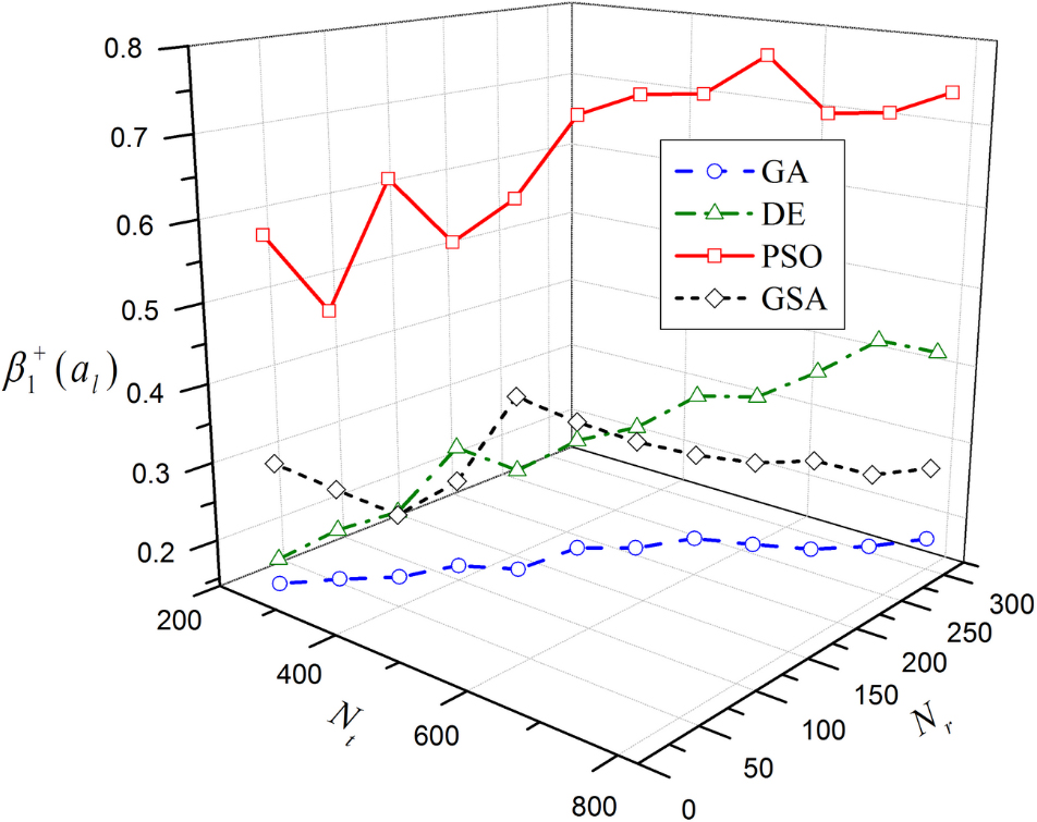
Figure 2.
Movement of the optimal
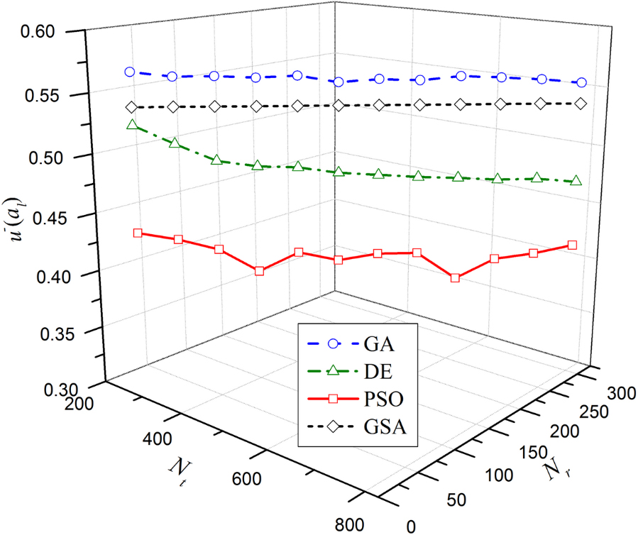
Figure 1 shows that with the increase in
As for the efficiencies of the four algorithms, Tables 9 and 10 show that
7.Conclusions
In the process of solving MCDM problems with IVBDs, individual IVBDs are explicitly combined to generate an aggregated IVBD or implicitly combined in the optimization model of generating the minimum and maximum expected utilities. For an MCDM problem with a large number of criteria and grades, implementing the accurate combination of IVBDs within an acceptable time is difficult. Evolutionary algorithms provide effective methods for overcoming this difficulty. When these algorithms are selected to combine IVBDs or generate the expected utilities by implicitly combining IVBDs, a new issue occurs: which algorithm is suitable for accurately combining IVBDs within an acceptable time? To address this issue, four representative evolutionary algorithms with many extensions and applications, including GA, DE algorithm, PSO algorithm, and GSA, are selected to explicitly and implicitly combine IVBDs. By performing experiments on combining IVBDs and generating the expected utilities, a comparative analysis of the four algorithms is provided with the help of two indicators: accuracy and efficiency. The analysis indicates that PSO algorithm is more suitable than the other three algorithms to combine IVBDs and generate the expected utilities. This conclusion is highlighted by a sensitivity analysis of the four algorithms’ accuracies and efficiencies.
In this paper, we only compare the original versions of the four evolutionary algorithms for analyzing MCDM problems with IVBDs. Whether the extensions of the four algorithms can improve their accuracies and efficiencies for combining IVBDs deserves consideration, and will be investigated in the future. In addition, for MCDM problems with other types of uncertain preferences, such as linguistic term set, intuitionistic fuzzy set, hesitant fuzzy set, and interval type-2 fuzzy set, it would also be interesting to compare the accuracies and efficiencies of the four algorithms for analyzing the problems.
Acknowledgments
This research is supported by the National Natural Science Foundation of China (Grant Nos. 71622003, 71571060).
References
[1] | He YD, He Z. Extensions of Atanassov’s intuitionistic fuzzy interaction Bonferroni means and their application to multiple-attribute decision making. IEEE Transactions on Fuzzy Systems. (2016) ; 24: : 558-573. |
[2] | Yu WY, Zhang Z, Zhong QY, Sun LL. Extended TODIM for multi-criteria group decision making based on unbalanced hesitant fuzzy linguistic term sets. Computers & Industrial Engineering. (2017) ; 114: : 316-328. |
[3] | He YD, He Z, Wang GD, Chen HY. Hesitant fuzzy power bonferroni means and their application to multiple attribute decision making. IEEE Transactions on Fuzzy Systems. (2015) ; 23: : 1655-1668. |
[4] | Wu XL, Liao HC. An approach to quality function deployment based on probabilistic linguistic term sets and ORESTE method for multi-expert multi-criteria decision making. Information Fusion. (2018) ; 43: : 13-26. |
[5] | Fu C, Chin KS. Robust evidential reasoning approach with unknown attribute weights. Knowledge-Based Systems. (2014) ; 59: : 9-20. |
[6] | Chen TY. Interval-valued fuzzy multiple criteria decision-making methods based on dual optimistic/pessimistic estimations in averaging operations. Applied Soft Computing. (2014) ; 24: : 923-947. |
[7] | Zhang WK, Ju YB, Liu XY. Multiple criteria decision analysis based on Shapley fuzzy measures and interval-valued hesitant fuzzy linguistic numbers. Computers & Industrial Engineering. (2017) ; 105: : 28-38. |
[8] | Tang XA, Fu C, Xu DL, Yang SL. Analysis of fuzzy Hamacher aggregation functions for uncertain multiple attribute decision making. Information Sciences. (2017) ; 387: : 19-33. |
[9] | He YD, He Z, Shi LX, Meng SS. Multiple attribute group decision making based on IVHFPBMs and a new ranking method for interval-valued hesitant fuzzy information. Computers & Industrial Engineering. (2016) ; 99: : 63-77. |
[10] | Wang JC, Chen TY. A simulated annealing-based permutation method and experimental analysis for multiple criteria decision analysis with interval type-2 fuzzy sets. Applied Soft Computing. (2015) ; 36: : 57-69. |
[11] | Fu C, Yang SL. An evidential reasoning based consensus model for multiple attribute group decision analysis problems with interval-valued group consensus requirements. European Journal of Operational Research. (2012) ; 223: : 167-176. |
[12] | Cheshmehgaz HR, Haron H, Kazemipour F, Desa MI. Accumulated risk of body postures in assembly line balancing problem and modeling through a multi-criteria fuzzy-genetic algorithm. Computers & Industrial Engineering. (2012) ; 63: : 503-512. |
[13] | Kaliszewski I, Miroforidis J, Podkopaev D. Interactive multiple criteria decision making based on preference driven evolutionary multiobjective optimization with controllable accuracy. European Journal of Operational Research. (2012) ; 216: : 188-199. |
[14] | Kapsoulis D, Tsiakas K, Trompoukis X, Asouti V, Giannakoglou K. Evolutionary multi-objective optimization assisted by metamodels, kernel PCA and multi-criteria decision making techniques with applications in aerodynamics. Applied Soft Computing. (2018) ; 64: : 1-13. |
[15] | Said LB, Bechikh S, Ghédira K. The r-dominance: A new dominance relation for interactive evolutionary multicriteria decision making. IEEE Transactions on Evolutionary Computation. (2010) ; 14: : 801-818. |
[16] | Wang R, Purshouse RC, Giagkiozis I, Fleming PJ. The iPICEA-g: A new hybrid evolutionary multi-criteria decision making approach using the brushing technique. European Journal of Operational Research. (2015) ; 243: : 442-453. |
[17] | Xue F, Sanderson AC, Graves RJ. Multiobjective evolutionary decision support for design-supplier-manufacturing planning. IEEE Transactions on Systems, Man, and Cybernetics - Part A: Systems and Humans. (2009) ; 39: : 309-320. |
[18] | Javanbarg MB, Scawthorn C, Kiyono J, Shahbodaghkhan B. Fuzzy AHP-based multicriteria decision making systems using particle swarm optimization. Expert Systems with Applications. (2012) ; 39: : 960-966. |
[19] | Kennedy J, Eberhart R. Particle swarm optimization. In Proceeding of IEEE International Conference on Neural Network, Perth, WA, Australia, Australia, (1995) ; 1942-1948. |
[20] | Chen SM, Huang ZC. Multiattribute decision making based on interval-valued intuitionistic fuzzy values and particle swarm optimization techniques. Information Sciences. (2017) ; 397-398: : 206-218. |
[21] | Wu H, Pang GK, Choy KL, Lam HY. A charging-scheme decision model for electric vehicle battery swapping station using varied population evolutionary algorithms. Applied Soft Computing. (2017) ; 61: : 905-920. |
[22] | Holland JH. Adaptation in Natural and Artificial Systems. University of Michigan Press, Ann Arbor, (1975) . |
[23] | Goldberg DE. Genetic Algorithms in Search, Optimization, and Machine Learning. Addison-Wesley, USA, (1989) . |
[24] | Storn R, Price K. Differential evolution-A simple and efficient adaptive scheme for global optimization over continuous spaces. Journal of Global Optimization. (1997) ; 11: : 341-359. |
[25] | Pei J, Cheng BY, Liu XB, Pardalos PM, Kong M. Single-machine and parallel-machine serial-batching scheduling problems with position-based learning effect and linear setup time. Annals of Operations Research. (2017) ; DOI 10.1007/s10479-017-2481-8. |
[26] | Pei J, Liu XB, Fan WJ, Pardalos PM, Lu SJ. A hybrid BA-VNS algorithm for coordinated serial-batching scheduling with deteriorating jobs, financial budget, and resource constraint in multiple manufacturers. Omega. (2019) ; 82: : 55-69. |
[27] | Rashedi E, Nezamabadi-pour H, Saryazdi S. GSA: A Gravitational Search Algorithm. Information Sciences. (2009) ; 179: : 2232-2248. |
[28] | Fu C, Xu DL. Determining attribute weights to improve solution reliability and its application to selecting leading industries. Annals of Operations Research. (2016) ; 245: : 401-426. |
[29] | Fu C, Xu DL, Yang SL. Distributed preference relations for multiple attribute decision analysis. Journal of the Operational Research Society. (2016) ; 67: : 457-473. |
[30] | Yang JB, Wang YM, Xu DL, Chin KS. The evidential reasoning approach for MADA under both probabilistic and fuzzy uncertainties. European Journal of Operational Research. (2006) ; 171: : 309-343. |
[31] | Xu DL. An introduction and survey of the evidential reasoning approach for multiple criteria decision analysis. Annals of Operations Research. (2012) ; 195: : 163-187. |
[32] | Yang JB, Xu DL. Evidential reasoning rule for evidence combination. Artificial Intelligence. (2013) ; 205: : 1-29. |
[33] | Jiang ZZ, Zhang RY, Fan ZP, Chen XH. A fuzzy matching model with Hurwicz criteria for one-shot multi-attribute exchanges in E-brokerage. Fuzzy Optimization and Decision Making. (2015) ; 14: : 77-96. |
[34] | Horvath E, Silva CF, Majlis S, Rodriguez I, Skoknic V, Castro A. Prospective validation of the ultrasound based TIRADS (Thyroid Imaging Reporting And Data System) classification: Results in surgically resected thyroid nodules. European Radiology. (2017) ; 27: : 2619-2628. |
[35] | Fu C, Yang SL. The conjunctive combination of interval-valued belief structures from dependent sources. International Journal of Approximate Reasoning. (2012) ; 53: : 769-785. |
[36] | Wang YM, Yang JB, Xu DL, Chin KS. On the combination and normalization of interval-valued belief structures. Information Sciences. (2007) ; 177: : 1230-1247. |
[37] | Wang YM, Yang JB, Xu DL, Chin KS. The evidential reasoning approach for multiple attribute decision analysis using interval belief degrees. European Journal of Operational Research. (2006) ; 175: : 35-66. |
[38] | Sharma SK, Irwin GW. Fuzzy coding of genetic algorithms. IEEE Transactions on Evolutionary Computation. (2003) ; 7: : 344-355. |
[39] | Charalampakis AE. Registrar: A complete-memory operator to enhance performance of genetic algorithms. Journal of Global Optimization. (2012) ; 54: : 449-483. |
[40] | Dao SD, Abhary K, Marian R. An innovative framework for designing genetic algorithm structures. Expert Systems with Applications. (2017) ; 90: : 196-208. |
[41] | Yang T, Kuo Y, Cho C. A genetic algorithms simulation approach for the multi-attribute combinational dispatching decision problem. European Journal of Operational Research. (2007) ; 176: : 1859-1873. |
[42] | Goletsis Y, Papaloukas C, Fotiadis DI, Likas A, Michalis LK. Automated ischemic beat classification using genetic algorithms and multicriteria decision analysis. IEEE Transactions on Biomedical Engineering. (2004) ; 51: : 1717-1725. |
[43] | Chang YH, Lee MS. Incorporating Markov decision process on genetic algorithms to formulate trading strategies for stock markets. Applied Soft Computing. (2017) ; 52: : 1143-1153. |
[44] | Das S, Abraham A, Chakraborty UK, Konar A. Differential evolution using a neighborhood-based mutation operator. IEEE Transactions on Evolutionary Computation. (2009) ; 13: : 526-553. |
[45] | Sarker RA, Elsayed SM, Ray T. Differential evolution with dynamic parameters selection for optimization problems. IEEE Transactions on Evolutionary Computation. (2014) ; 18: : 689-707. |
[46] | Brest J, Greiner S, Bošković B, Mernik M, \̌refauthor{\snm{Z}umer} \fnms{V}. Self-adapting control parameters in differential evolution: A comparative study on numerical benchmark problems. IEEE Transactions on Evolutionary Computation. (2006) ; 10: : 646-657. |
[47] | Qiu X, Xu JX, Tan KC, Abbass HA. Adaptive cross-generation differential evolution operators for multiobjective optimization. IEEE Transactions on Evolutionary Computation. (2016) ; 20: : 232-244. |
[48] | Santucci V, Baioletti M, Milani A. Algebraic differential evolution algorithm for the permutation flowshop scheduling problem with total flowtime criterion. IEEE Transactions on Evolutionary Computation. (2016) ; 20: : 682-694. |
[49] | Zhong JH, Shen M, Zhang J, Chung HS, Shi YH, Li Y. A differential evolution algorithm with dual populations for solving periodic railway timetable scheduling problem. IEEE Transactions on Evolutionary Computation. (2013) ; 17: : 512-527. |
[50] | Bonyadi MR, Michalewicz Z. Stability analysis of the particle swarm optimization without stagnation assumption. IEEE Transactions on Evolutionary Computation. (2016) ; 20: : 814-819. |
[51] | Bonyadi MR, Michalewicz Z. Impacts of coefficients on movement patterns in the particle swarm optimization algorithm. IEEE Transactions on Evolutionary Computation. (2017) ; 21: : 378-390. |
[52] | Chen KH, Wang KJ, Wang KM, Angelia MA. Applying particle swarm optimization-based decision tree classifier for cancer classification on gene expression data. Applied Soft Computing. (2014) ; 24: : 773-780. |
[53] | Zheng YJ, Ling HF, Xue JY, Chen SY. Population classification in fire evacuation: A multiobjective particle swarm optimization approach. IEEE Transactions on Evolutionary Computation. (2014) ; 18: : 70-81. |
[54] | Palafox L, Noman N, Iba H. Reverse engineering of gene regulatory networks using dissipative particle swarm optimization. IEEE Transactions on Evolutionary Computation. (2013) ; 17: : 577-587. |
[55] | Haghbayan P, Nezamabadi-pour H, Kamyab S. A niche GSA method with nearest neighbor scheme for multimodal optimization. Swarm and Evolutionary Computation. (2017) ; 35: : 78-92. |
[56] | Chakraborti T, Chatterjee A. A novel binary adaptive weight GSA based feature selection for face recognition using local gradient patterns, modified census transform, and local binary patterns. Engineering Applications of Artificial Intelligence. (2014) ; 33: : 80-90. |
[57] | Barani F, Mirhosseini M, Nezamabadi-pour H, Farsangi MM. Unit commitment by an improved binary quantum GSA. Applied Soft Computing. (2017) ; 60: : 180-189. |
[58] | Chen Z, Yuan X, Tian H, Ji B. Improved gravitational search algorithm for parameter identification of water turbine regulation system. Energy Conversion and Management. (2014) ; 78: : 306-315. |
[59] | Bottomley PA, Doyle JR. A comparison of three weight elicitation methods: Good, better, and best. Omega. (2001) ; 29: (6): 553-560. |
[60] | Roberts R, Goodwin P. Weight approximations in multi-attribute decision models. Journal of Multi-Criteria Decision Analysis. (2002) ; 11: (6): 291-303. |
[61] | Takeda E, Cogger KO, Yu PL. Estimating criterion weights using eigenvectors: A comparative study. European Journal of Operational Research. (1987) ; 29: (3): 360-369. |
[62] | Rezaei J. Best-worst multi-criteria decision-making method. Omega. (2015) ; 53: : 49-57. |

