
Deep learning models for predicting the position of the head on an X-ray image for Cephalometric analysis
Abstract
Cephalometric analysis is used to identify problems in the development of the skull, evaluate their treatment, and plan for possible surgical interventions. The paper aims to develop a Convolutional Neural Network that will analyze the head position on an X-ray image. It takes place in such a way that it recognizes whether the image is suitable and, if not, suggests a change in the position of the head for correction. This paper addresses the exact rotation of the head with a change in the range of a few degrees of rotation. The objective is to predict the correct head position to take an X-ray image for further Cephalometric analysis. The changes in the degree of rotations were categorized into 5 classes.
Deep learning models predict the correct head position for Cephalometric analysis. An X-ray image dataset on the head is generated using CT scan images. The generated images are categorized into 5 classes based on a few degrees of rotations. A set of four deep-learning models were then used to generate the generated X-Ray images for analysis. This research work makes use of four CNN-based networks. These networks are trained on a dataset to predict the accurate head position on generated X-Ray images for analysis. Two networks of VGG-Net, one is the U-Net and the last is of the ResNet type. The experimental analysis ascertains that VGG-4 outperformed the VGG-3, U-Net, and ResNet in estimating the head position to take an X-ray on a test dataset with a measured accuracy of 98%. It is due to the incorrectly classified images are classified that are directly adjacent to the correct ones at intervals and the misclassification rate is significantly reduced.
1.Introduction
Cephalometric analysis is the process of diagnosis and treatment of problems in the development of the skull, evaluating their treatment, and planning for possible surgical interventions. Cephalometry is an examination of the connections between the skeletal and dental structures of the human skull. Oral and maxillofacial surgeons, orthodontists, and dentists regularly use it as a method for planning therapy. Cephalometric analysis is used to examine the facial anatomical links and measure facial progression. Cephalometric evaluation is a procedure that is intrinsically flawed because it is based on either sagittal or coronal plane 2D radiography images. Routine 3D examination of facial morphology is now possible thanks to the widespread methods for 3D imaging that are readily available, such as computed tomography and magnetic resonance imaging. With 3D Cephalometry, longitudinal growth, and craniofacial morphology may be measured with more accuracy, and it may also be possible to spot small occlusion changes. Through 3D skull alignment, an accurate and landmark-free evaluation of the true symmetry of the head is generated. It enables the cranium to be accurately aligned with predetermined markers.
For Cephalometric analysis, it is necessary to determine the boundaries or landmarks on the side X-Ray of the head. These landmarks tell us about the skull and jaw’s future development and current state. Detection of these boundaries is the first step in Cephalometric analysis [14]. Cephalometric analysis obtains this information from the evaluation of relations between boundaries. These relationships include for example, distances or angles. Turning the head at the time of analysis can affect the relationships between the designated boundaries and thus invalidate or even change the diagnosis [13]. Most methods that perform this analysis either do not check the quality of the analyzed image or if they do, only briefly. The risk of misdiagnosis is high if the Cephalometric analysis is performed automatically. The nasion’s, subnasale’s, and gonion’s forward projection are determined using Cephalograms. Additionally, it establishes how various horizontal face levels relate to the base of the skull. To effectively treat hemifacial microsomia, it is crucial to determine the link between the horizontal occlusal plane and the skull base using Cephalometry (HFM). If Cephalometry is misdiagnosed it shows an effect on the side profile of the face view, miscorrelation between the jaw and the cheekbone, misleading the information about malocclusions. These distorted results of such could ultimately prevent and endanger the patient’s problem.
![Example of cephalometric X-ray image with landmarks [11].](https://content.iospress.com:443/media/ida/2023/27-S1/ida-27-S1-ida237430/ida-27-ida237430-g001.jpg)
The presented work deals with the validation and possible proposal for correcting Cephalometric images. Cephalometric images, in this case, are X-Rays of the patient’s head as shown in Fig. 1. A human error occurs during scanning and the patient may move his head and degrade the image. This work aims to determine whether a Cephalometric analysis can be performed on the image, which demands the accuracy of determining certain points in the image. Because of this, digital X-rays taken using computed radiography (CR) are adopted [24]. To release the trapped energy as light with an X-ray intensity proportional to it, CR employs a storage phosphor that needs light input. The digital X-ray image produced with landmark identification done using deep learning methods as shown in Fig. 2, it is important that the image is good and that the patient’s head is in the correct position when taking the X-Ray [15]. If the image is degraded, the program will recommend rotating the patient’s head a certain number of degrees for correction [18]. A relatively large unknown is finding the boundary that separates valid from invalid images. No general rule determines which head rotation is still acceptable and which is no longer. On the contrary, the ideal rotation varies depending on what it tries to find out from the image.
![Example of Cephalometric Landmark Analysis [11].](https://content.iospress.com:443/media/ida/2023/27-S1/ida-27-S1-ida237430/ida-27-ida237430-g002.jpg)
Four convolutional Networks were created and trained to achieve the desired result. Each of them is inspired by its design and proven architecture. These architectures have been implemented and modified to suit the intentions of this work. In each experiment, certain metrics were measured that characterize the capabilities of the trained network. Depending on the measured values, the parameters of other experiments are adjusted.
A dataset was created for training and testing networks. This division is important because the accuracy of the training data can be misleading. The actual accuracy of a network is measured on data that the network did not encounter during training. The dataset had to be artificially generated from CT scans due to the lack of freely available resources. Images are available, but only those that are suitable for Cephalometric [11]. This means that the available datasets represent only a part of the frames that want to be recognized in the network. All images were divided into classes that correspond to the degree of rotation of the head in the image.
Images in similar categories are mainly interchanged. And it is not so important whether the program recommends correcting the head rotation by 5
The second section deals with the theoretical basis and related work, used in this work. The creation and division of the dataset are contained in Section 3. A description of the architecture designed and implemented is described in Section 4. The method of experimentation and the measured results on the networks can be found in Section 5.
2.Basic preliminaries and related works
2.1Artificial neural networks
An artificial neural network is a model very often used in the field of computer science, which deals with artificial intelligence. The neurons are interconnected, and each neuron adjusts and passes on the signal [1]. The remaining problem is how to set up individual l neurons’ transformations so that the resulting information is the same as expected. These weights are adjusted during the learning phase. Learning differs between learning with a teacher and learning without a teacher. In the case of teacher learning, inputs are presented to the network, the neural network processes the input, then the results from the network are compared with the correct results, and the weights are adjusted accordingly in the network to make the results more similar to the actual ones [21].
2.2Activation functions
The activating function is part of the neuron that creates nonlinearity in the neuron’s output. This is important because if there were no activating function in a neuron, the network would only be able to solve trivial problems. Using activation features allows smaller networks to compute more complex issues.
2.2.1Sigmoid and hyperbolic tangent
These functions are similar; the difference is in the range of values. They are mainly used on output layers, use on hidden layers is not highly recommended because the scope of their domain makes it difficult to learn the network. The prescription of sigmoid [10] is:
(1)
The prescription of the hyperbolic tangent [3] is:
(2)
The two major problems with sigmoid activation functions. Sigmoid saturates and kills the gradients and is not zero-centered. To overcome the saturation problem ReLU function is used.
2.2.2Rectified Linear Unit (ReLU)
ReLU is the activation method in neural networks that is most frequently utilized [10]. ReLU is similar to a linear function but retains some of the advantages of linear functions. The benefits of using this activation function are easy gradient propagation and efficient calculation. This feature can only be implemented using compare, add, and multiply operations. The prescription for this function is:
(3)
ReLU has a problem known as the dying ReLU’s when certain neurons essentially stop producing anything other than 0 throughout training. Gradient descent has no effect, as it simply continues to output 0. Another restriction is the possibility of neuron death when weights are adjusted to the point where all instances in the training set are negative.
2.2.3Softmax
Softmax is a function that normalizes the output of a neural network so that the sum of all the values of output neurons gives 1. In this way, the probability that the network input data belongs to the given category is determined. This function is similar to sigmoid; the output is also between 0 and 1, but the difference is that the noise level is normalized [17].
2.3Topology
Topology, when talking about neural networks, means their arrangement. In the case of a forward neural network, each neuron feeds its output to the input of each neuron in the next layer. The interconnection of individual neurons forms something like a network, hence the name “neural network” [21].
2.3.1Fully interconnected forward layer
A fully interconnected anterior layer is an arrangement of neurons, each neuron having at the input the output of each neuron of the previous layer. This layer is context-independent; past inputs do not affect the current state [16]. Neurons in the same layer are not connected; the signal propagates in one direction.
2.3.2Recurrent layer
Neurons can perceive past and future information in the same way because consider the input’s time context. The output from this layer is fed to the input of the same layer when processing the next input. In this way, the neural network can perceive past inputs.
2.3.3Convolution layer
This layer is mainly used for image recognition. This layer is one of the main components of all the architectures used in this work. The input to this layer is an n-dimensional array, and the output is as well. Each feature map results from applying a convolution filter to the input. The size of the filter indicates how many weights must be trained within this filter. Filters typically have symmetrical dimension sizes and two-dimensional filters are generally used to recognize the image. Filters with odd sizes have proved successful in practice, so looking at the application of convolution layers will see mainly filter dimensions of 3x3 and 5
2.3.4Pooling layer
The function of the pooling layer is to reduce the space, reduce the input to other layers of the network, and thus reduce the number of parameters that need to be trained. This layer has 2 parameters, the first is the core size, and the second is the offset step. The kernel size determines the size of the space from which the new values will be selected. The scroll step determines how much the kernel will scroll. The smaller the core, the more detail it can preserve. Layer pooling is divided into max-pooling and average pooling according to the selection of values from the kernel space. Max-pooling layers select the highest values from the space and pass them to their output. Average-pooling layers have a different strategy of choosing the output value, averaging the entire kernel space, and passing it to the output [3].
2.4Batch normalization
Batch normalization is used so that the network does not stop learning. This happens mainly in deep networks, where the signal is multiplied repeatedly. The signal may get to a state where it disappears or increases to too high values, and the network then stops learning. It helps prevent these problems by subtracting the batch average from each dimension and dividing it by the batch standard deviation. The optimizer can change these parameters in the next layer to reduce the loss function [8].
2.5Residual joint
Residual connections are used in deep neural networks. Its goal is to optimize the depth of the network so that layers that are not needed are not unnecessarily learned. This connection works by adding the input to the block the output of the previous block with the block before the previous one [6].
2.6Dropout layer
The dropout layer is used to reduce network overtraining. When a signal propagates through this layer, many elements are deactivated. As a result, the network forgets certain qualities that it has learned during training. This prevents neural networks from overtraining and improves performance [16].
2.7Training
The motivation for training a neural network is to find the smallest possible sum of deviation and variance. Variance is minimal at the beginning, so try to grow as little as possible during training. This process will end the training at the moment when the sum of disruption and variance is minimal. Training can be thought of as the propagation of a signal through a neural network and the subsequent adjustment of the weight vectors of each neuron using an error backpropagation algorithm. This is done several times until it gets the feeling that the sum of the deviation and variance is minimal.
During training, the data is usually divided into training and validation. This division is used to check if the network is being over-trained. The error is also measured on the validation set, and when this error stops decreasing, it is appropriate to end the training [4]. Training and validation are the two most important areas of data analysis for a machine-learning program, and they are done on a batch-by-batch basis to ensure that the scales are not adjusted after each input, but only after the entire batch. This prevents overtraining and significantly speeds up the learning process of the neural network because each input within the batch can be processed in parallel. The batch size must be selected depending on the entire training dataset’s size and the hardware capabilities on which the network is trained.
3.The process of X-ray image generation
3.1Dataset description
The dataset for this task was created from CT images taken from SICAS Medical Image Repository [22]. Medical research data at SICAS Medical Image Repository contains medical images of the skull, surface models, genomics data, clinical data, and statistical shape models are all available in the openly accessible [22]. The information can be shared and made openly available on SMIR. The SICAS offers a special blend of proficiency in data processing and data visualization for use in medical research and applications, as well as in the acquisition and storage of medical pictures. The information stored in SICAS has the features like Anonymization, Data Storage, Research expertise, Acquisition, Controlled, and Anatomy. While CT scan images are in 3D, and the X-ray images are in 2D. Despite how little there is a difference between a CT image and an X-ray, it matters. X-rays are used by pathologists to recognize pneumonia and cancer as well as bone fractures and dislocations. However, using X-ray images of the structure, CT scans, an advanced X-ray technology, are used to diagnose internal organ injuries.
The process of generating an X-ray dataset from CT images is described in Section 3.2. The basic dataset for this research contains 1157 CT scan images of the head taken from [22]. The dataset for training the networks was artificially generated images from CT scans. After this expansion, the dataset contained 1957 head images. The training data includes 1867 and the test data contains 90 images. In artificially generated images, the training data is divided into 5 categories according to the level of head rotation at the time the image was taken. Real X-rays are only part of a category indicating zero or little head rotation because they usually have no practical value in storing for medical purposes. Figure 3 shows the specimen of generated X-Ray image from the CT image. For this reason, it was necessary to generate the rest of the categories from CT scans of the entire head. The whole dataset is divided into 5 categories. A valid image with a deflection of
Figure 3.
Comparison of the actual image with the generated image.
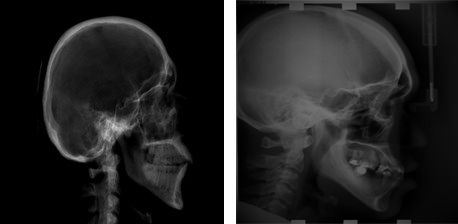
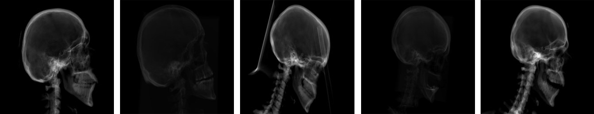
Figure 4.
Images of classes
3.2Generation of X-rays images from CT scans
To expand the dataset and thereby achieve better results in neural training networks, a program was created for the artificial generation of images [23]. This program reads the 1157 CT scan images of the head taken as a series in DICOM format and displays them as a 3D model. DICOM is Digital Imaging and Communications in Medicine, which includes a scanned image, such as an ultrasound or CT (Computed Tomography) scan image. The metadata of DICOM files may also contain patient identity information. Visualizers that accept this data allow users to see and open images stored in this format [24]. DICOM format is used to measure the radio density using a Hounsfield unit. The Hounsfield unit provides the relationship between grayscale value and organ density (HU). Radio density is quantitatively scaled using the Hounsfield Unit (HU) system. The radio density of distilled water at standard pressure and temperature is transformed linearly (STP). Metadata, in the form of tags, is present in every DICOM file. Tags keep track of information on the patient, the process, the camera used to take the photo, and many other things. It uses different DICOM readers for the files.
A set of X-rays images are created using CT images [24]. The source of X-rays spins around the internal system of the CT imaging system as the patient moves through it. A portion of the patient’s body is exposed to X-rays from the X-ray source in the form of a narrow, fan-shaped beam. The fan beam can be made with a thickness ranging from 1 millimeter to 10 millimeters. A standard examination is performed in phase wise and the x-ray tube rotates around the patient. At one angle or rotation, the X-ray system will capture an “X-ray snapshot” of the patient’s exposed portion of the body. Multiple “snapshots” (angles) are gathered throughout a revolution. The data is supplied to the computer for each full rotation of the X-ray source, and it subsequently reconstructs each distinct “snapshot” into a cross-sectional image of the organs and tissues.
This program has been modified for the needs of this work. The program first loads the images that are sections created during the CT scan in DICOM format. A 3D model of the entire head is created and drawn. A volume ray casting in combination with additive bending is used to achieve the X-ray effect. The model can rotate, move, and zoom in and out so that only the part of the body from which it is taken takes a picture. The brightness and contrast of the model can also be changed to bring it closer to the real X-ray image. When a certain number of degrees rotate an X-ray model, a series of simulation images are created. The images are stored in a folder that matches their category. A different number of frames are created by rotating the model for each category. The number of frames per category is estimated so that the representation of the category in the entire dataset corresponds to the percentage of the actual deployment of the program. This system is not completely accurate. For example, the representation of the category 20
Finding the ideal position with zero rotation is also a problem for the analysis. Such a position is not easy to define, because each person has certain specifics regarding the shape of the skull. When generating, I followed the rule that the ideal rotation is one where the paired structures of the brain’s skull are not seen twice but overlap. A perfect image is determined by dividing the dataset into classes, such that all the points in the spectrum are within a certain distance from each other. Of course, this cannot be done perfectly, because some may overlap and others may not, and there is no angle where they all overlap.
3.3Volume ray casting
The term “volume rendering” describes techniques that make it possible to visualize 3D data. The 3D spatial dimensions are rendered into 2D projections of a colored, semitransparent volume computed as sampled function. Computed Tomography (CT) contains an array of X-ray absorption coefficients. Compared to traditional X-rays, CT pictures have the benefit of containing data from all planes rather than just one. The Ray Casting method, also known as “backward mapping,” is used for volume rendering. Ray casting does not try to impose any geometric form on the three-dimensional data, allowing for the optimum utilization of the data. It addresses significant issues with surface extraction methods, specifically the way they project a thin shell in the acquisition region. An algorithm for rendering image-ordered volumes is ray-casting. The fundamental concept is to send an array of rays through the pixels in an image plane to ascertain the pixel values. The beams gather RGBA coefficients along the route and for display blend them for display in RGBA visualization format. The Ray-casting visualization can be used with a variety of techniques to produce a wide range of perspectives of the same image.
Volume Ray casting is a technique that allows the projection of a 3D model into 2D. This is used to display our simulation of an X-ray image from a CT scan [25]. The CT scan is here in the form of the following sections, forming a three-dimensional model. Volume Ray casting is an algorithm where beams are emitted toward the 3D model we want to display. In our case, from the camera’s location, in a 3D world, this is the position from which we want our model to be viewed. These rays pass through the model, creating patterns in RGBA color. This color is then calculated from all samples, and the currently processed pixel will be rendered on the display plane. In this way, the color of each pixel and thus the image wanted to be induced can be identified [9]. Figure 5 shows the principle of volume ray casting.
![Principle of volume ray casting. Source [26].](https://content.iospress.com:443/media/ida/2023/27-S1/ida-27-S1-ida237430/ida-27-ida237430-g005.jpg)
3.4Additive blending
Blending is the process of mixing two colors to produce a third color. In the actual world, blending occurs frequently as light travels through glass reflects off surfaces, and superimposes a light source on a background, like a flare that surrounds a streetlight at night. By including a blending mode, you can change how the colors on a layer interact with the colors on lower layers. Simply altering the blending modes will change how your illustration looks. The three consecutive steps of a blending process are typically loading and weighing the blend components, mixing, and discharging the finished result.
3.4.1Three types of blending
• Additive blending: When we combine many hues and then add the outcome, we are doing additive blending. Since monitors are merely combining three different primary colors, this is how our vision and light interact to give us the perception of millions of various colors.
• Multiplicative blending: Another helpful blending mode that simulates when light enters our eyes after passing through a color filter or bouncing off a lighted object is multiplicative blending commonly referred to as modulation. When white light touches a red object, blue and green light is absorbed, giving the thing its red appearance to us. Our eyes only receive reflections of red light. We might observe a surface that reflects some red and some green but very little blue in the example on the left. When multi-texturing is not possible, Multiplicative blending is used to generate light maps in games. The light map is multiplied by the texture to fill in the areas that are lighted and shadowed.
• Interpolative blending: The interpolative effect can be created by combing the Multiplicative and Additive in interpolative blending. In some cases, the effects of this blending mode will only be accurate if you draw the furthest translucent objects first and the closest ones after. This is different from addition and modulation by themselves. Triangles can overlap and cross, so even sorting wouldn’t be ideal, but the resulting artifacts would be acceptable. Interpolation can be used to create effects like tinted glass or fade-in/fade-out as well as to blend adjacent surfaces. Two textures are interpolated together in the image on the left.
Additive blending is used to create pixel colors from individual samples that belong to a pixel. It is based on the fact that the resulting pixel color will be the sum of the colors of all samples. In combination with Ray casting the resulting color of each pixel was calculated. Figure 6 shows the sample image generated on
Figure 6.
Generated image on
The objective of our research is to fix the degree of rotation in the skull image for accurate diagnosis. Although the difference between an X-ray image and a CT scan is minor, it is very significant in detecting landmarks. Pathologists use X-rays to identify pneumonia and cancer, as well as fractures and dislocations of bones. However, using X-ray images, a CT scan, is used to identify injuries in the inner organs. While CT images are in 3D, X-rays are in 2D. 2D images of a person’s body are taken from different angles as the CT scanner rotates around an axis. To detect the presence of an injury or disease, the computer combines all the cross-sectional photos and displays them on a screen as a 3D representation of the inside of the body. This examination can be extended as with CT scans for Cephalometric analysis.
4.Design of VGG based CNN model for predicting the position of the head on an X-ray image for Cephalometric Analysis
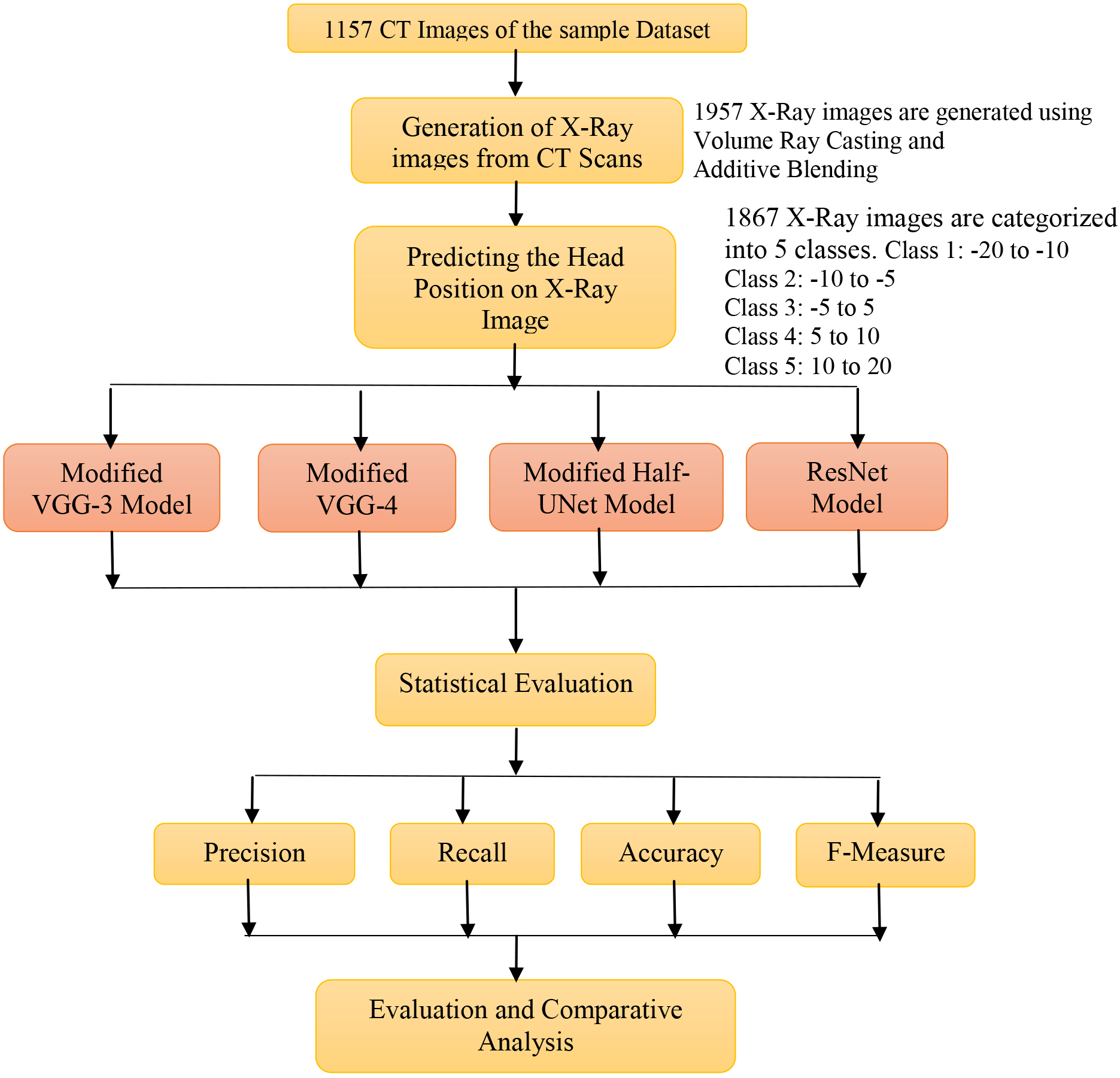
In this experiment, CT scan images are used to create an X-ray image dataset of the head. The accurate head position on the generated X-Ray image for Cephalometric analysis is predicted using four deep-learning models. The methodology of the proposed research work is shown in Fig. 7. As stated, modified Convolutional network architectures [5] were used in this work. This section will describe here exactly how they were modified.
Figure 7.
Flowchart of the proposed approach.
4.1VGG-network
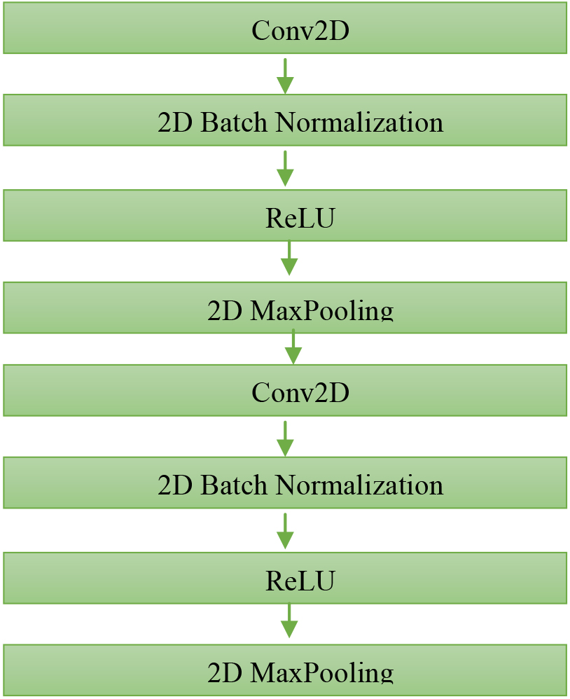
VGG is one of the best-known architectures in image data classification and analysis [16]. Layers alternate in it, which are divided into blocks. Each block entails a Conv_2D layer, batch normalization, a ReLU activation function, and a Max-pooling layer as shown in Fig. 8. This combination is repeated twice in each block as shown in Fig. 9. The same blocks as in VGG networks are used for subsampling. There are several blocks in a row, followed by one or more linear layers, which form a vector at the output, indicating the evaluation of the probability that the image fits the given class.
![VGG-Net architecture [10].](https://content.iospress.com:443/media/ida/2023/27-S1/ida-27-S1-ida237430/ida-27-ida237430-g008.jpg)
Figure 9.
Basic VGG Block structure for image analysis.
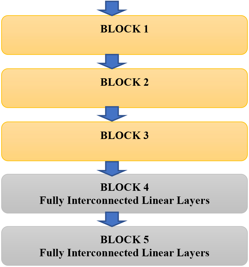
4.2VGG-3 network
This network is an implementation of the VGG network. It consists of three blocks connected in series as shown in Fig. 10. These three blocks are followed by two fully interconnected layers. It is interesting to monitor the development of the number of channels in the network passage. In this, the input to the first block is three channels; each representing one of the colors, and the output is eight channels. The eight channels are logically the inputs to the second block. The second block expands the number of channels to 16 and the third block to 32. The subsequent linear layers narrow and the last layer already has an output size that corresponds to the classifications and calculates the cross-entropy error function. This is an example of a deep neural network, which learns faster and is not as prone to overtraining as larger networks. In practice, it means that it learns faster because fewer scales can be set – but it may not be able to recognize small details as well as deeper networks.
Figure 10.
VGG-3 architecture.
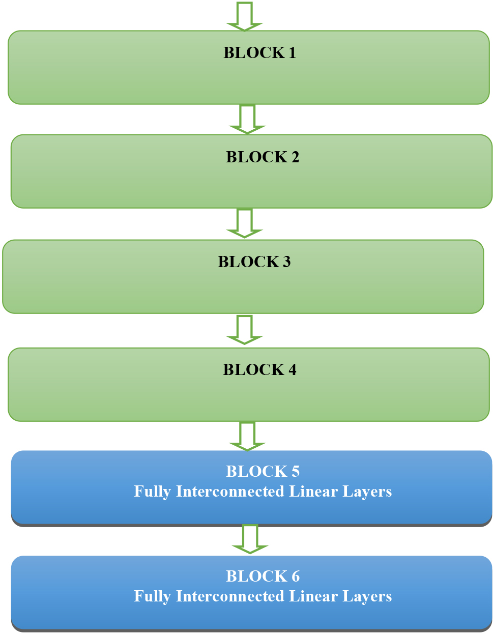
4.3VGG-4 network
VGG-4 is an intermediate stage between a simple VGG-3 network and deeper and more complicated networks. Here, too, the Cross-Entropy function is used to calculate the training error. The number of channels in the blocks is the same as in VGG-3, except that the last block outputs 64 channels. They differ practically only in their depth because VGG-4 consists of 4 blocks shown in Fig. 11 compared to VGG-3, where there are only 3. This fact also affects the resulting number of channels from the last block.
Figure 11.
VGG-4 architecture.
4.4Half-UNet
U-Net is a Convolutional neural network architecture premeditated to work with biomedical images [12]. The first part is a simple VGG-a network that subsamples the input. The other part, on the other hand, up samples the signal until it has the same shape as the network input. In U-Net, a Rectified Linear Unit (ReLU), two 3
U-Net is not the same as the single hourglass model. A convolutional neural network with a single hourglass-shaped design [15, 16] has two stages: an encoder stage and a decoder stage. Six blocks make up the encoder, each of which has a convolutional layer, a batch normalization module, and a max-pooling layer. In contrast, the six blocks that make up the decoder each have an up-sampling block, notwithstanding max-pooling. Filter kernels of size 33 are used to create a set number of convolutional layers. Per the convolutional layer, 128 kernels are taken into account in the current investigation. Up sampling takes place in the decoder stage, whereas downsampling takes place in the encoder stage, where the image size is reduced after each block. The network’s output is utilized to locate landmarks. Due to this, U-Net varies from the single hourglass model in that it outputs the output from both the upper and lower subsampling layers.
U-Net was designed specifically for medical image recognition and strived to preserve the features that are appropriate for this job while modifying the architecture to best suit our purpose. Half-UNet is inspired by U-Net architecture, which tries to use the preservation of outputs of higher layers of the network, such as biomedical data. The suggested architecture is a network of encoders and decoders same as in the U-Net topology. The Half-UNet is shown in Fig. 12. The redesigned architecture benefits from the integration of Ghost modules, full-scale feature fusion, and channel numbers. All feature maps in the channel numbers are unified in Half-UNet, which diminishes the size of the filter required for the convolution operation and helps the decoder’s feature fusion by removing the requirement for additional 3
![Half-UNet architecture [24].](https://content.iospress.com:443/media/ida/2023/27-S1/ida-27-S1-ida237430/ida-27-ida237430-g012.jpg)
The problem with the U-Net architecture and why it cannot be used here is that the size of its input corresponds to the output. In this paper, the output is in the form of categorization, and the network output layer must correspond. Specifically, this is the first part that subsamples the input. This is useful when a network highlights part of the image or finds some objects in it, but not for categorization.
Conversely, the part about that up samples was omitted. The difference compared to the VGG model is that the outputs from the higher layers of the network are preserved and fed to the input of the fully interconnected forward layers, which are located behind the Convolution layers, together with the input from the immediately preceding layer. The same blocks as in VGG networks are used for subsampling. A U-Net architecture with 4 blocks and 3 linear layers is used. The blocks are arranged one after the other, followed by linear layers. The output of the first block is fed to the input of the second and, at the same time, to the input of the last linear layer. In the same way, the output of the second block is fed to the input of the third block and the second linear layer. The output of the third block is connected in the same way. The output of the last block is connected to the input of the first linear layer [17, 20].
4.5ResNet
ResNet or Residual Neural network [6], solves the problem of fading signals, which often occurs in architectures with great depth (a large number of consecutive layers). The problem of the fading signal is caused by the repeated multiplication of the signal by small weight values, which results in low values in the low layers of the network being close to zero. ResNet uses the possibility of skipping a certain part of the network, where the output from the higher layer of the network is added to the input. In addition to the fading signal, this architecture also optimizes the learning speed of the network, as the network can bypass some layers, thus restoring signal strength.
The ResNet network was used mainly due to the feature given to it by the connection of the residual block. The dataset used is only training data and is relatively small; there is a high risk of overtraining. Overtraining occurs when a deep learning model can accurately predict training examples but is unable to generalize to fresh data. Overtraining occurs if the neural network is too powerful for the current problem. This leads to poor performance in the field. This typically happens when there is insufficient or homogeneous data. Inadequate model adjustment may have an impact on the data. Due to its potential to cause overconfidence and premature deployment, overtraining can be especially detrimental.
The ResNet, on the contrary, will avoid the problem of overtraining and works well with small data. Another advantage and simplification of implementation are that the PyTorch library includes an already implemented ResNet architecture model. Pre-training is training the network on another, often very large dataset. Although this training will not improve the accuracy of our problem, it significantly speeds up the training process. The library even offers 6 ResNet networks, which differ in size. Pre-training on a similar dataset can substantially speed up the training process because the scales in the network will only need to be adjusted a little [2]. Although this training will not improve the accuracy of our problem, if this large dataset has at least some resemblance to our dataset, the weight setting will not be completely random, but in some way already present.
5.Performance evaluation and experimental analysis
This section describes the methods and results of experiments on the implemented architectures. Specifically, the learning rate and the number of variables are changed for each architecture epoch and observed behavior during training and testing. There are mainly three indicators that are appropriate to change the network. This is a development of the error function values, the evolution of the accuracy of the test data, and the resulting accuracy of test data. Together, these values tell us if the network is over trained or undertrained and if we have too big or too little learning rate. If the accuracy of the test data does not improve in the long run, it may mean that the network has a low learning rate and is stuck at the local minimum of the error function. This can be solved by reducing the number of epochs. If consistently high training accuracy and insufficient test data mean that the neural network is re-learned and loses the ability to generalize.
5.1Implementation
As part of the implementation, four deep learning networks are designed and trained based on the architectures described in Section 4. Some of these architectures have been modified to suit our research better. The convolutional architectures of neural networks are designed for image recognition and are assembled in a way that the output builds the image again. This means that the output layer is for our work where we only need classification in one of the categories.
The learning rate is another important factor and must be chosen carefully to train the network correctly. If the learning rate is too large, the network will get stuck in local minima and diverge from the correct result. Fortunately, the training of the networks proposed in this work is significantly shorter; all training took place within tens of minutes. An important part of training is to determine the number of training epochs. An epoch is one training iteration where every image from the batch is the input. If the amount of training is too small, the network will not have enough options with the desired properties to learn. Overtraining arises due to exposure network to the same images too many times during the training phase.
The experimental analysis is carried out with the help of the Numpy library and Matplotlib. It uses PyTorch, which works with neural networks and optimization on the graphics card. A measure model script is used to measure the classification accuracy of individual classes of the trained model.
5.2Evaluation measures
Multiple metrics are used to evaluate the success of a network [19]. Using different metrics for different tasks is useful to represent the network’s ability to solve a given problem. The evaluation metrics can use true positive (TP), false positive (FP), true negative (TN), and false negative (FN).
5.2.1Accuracy
The accuracy [19] ratio of correctly classified images to the total number of images can be calculated as
(4)
5.2.2Precision
Precision [19] determines with what precision the network places images in the positive category. Precision is calculated as follows:
(5)
5.2.3Recall
Recall [19] indicates how many positive images the network recorded. The recall is calculated as:
(6)
5.2.4F-measure
F-measure [19] is a combination of Precision and Recall. The calculation is as follows:
(7)
5.3Statistical evaluation results
The generated X-Ray Images are distributed into training data and test data. The training dataset has 1867 images in all categories, while the test dataset has 90 images. To achieve this, the dataset was divided into 5 classes, each corresponding to a range of head rotations. We propose a much finer division of intervals than for the stages, which will occur only in the very minimum of cases.
During an epoch, the model is trained with the training data for one cycle. The training data and its associated information will be used once within an epoch. The database is portioned into one or more batches and the model is trained for each epoch using the portioned batch size. The epoch refers to the progression of going through the training instances of each batch. The size of the batch determines how many epochs there will be. For each epoch, the amount of data points is simply determined by multiplying the required iterations by the batch size. We can experiment using different epochs. In this case, the neural network is fed the same data several times. The essential structure of the data should be able to be represented by a decent model. In other words, it neither fits too well nor too poorly. Before training begins, we set the number of epoch parameters while creating a model. The primary elusive to us is to fix the number of epochs based on the batch size. With the intricate design of the neural network and the data collected, we must decide the point at which the weights converge.
Table 1
Division into classes by rotation
| Class_1 | Class_2 | Class_3 | Class_4 | Class_5 |
|---|---|---|---|---|
| 5 | 10 |
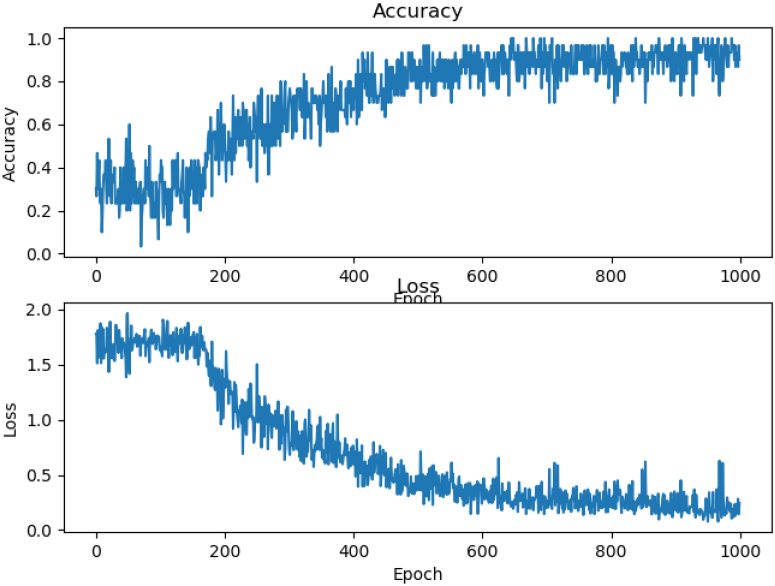
Figure 13.
Accuracy and Loss measure performance comparison on training result on VGG-3 Network for 1000 epochs.
Many factors affect a model’s accuracy, including weights, bias, and number of hidden layers, the type of activation function used, and hyperparameters like learning rate, batch size, and epoch count. When a model is trained, hyperparameters like learning rate, which are static variables and can be thought of as constants chosen by the practitioner beforehand, remain constant. Before using a learning algorithm on a dataset, we must set a variable for the learning rate. Before the training begins, the values are initialized to a lower value. The values are changed to reflect values that generate the intended outcomes. Since the learning rate is a parameter for the optimizer, we will test various learning rate values with various optimizers to observe how they affect the performance of the model. As a result, several learning rate values are chosen by hand-adjusting them until a pattern is discovered for each optimizer.
Figure 14.
Accuracy and Loss measure performance comparison on training data on VGG-3 Network for 10000 epochs.
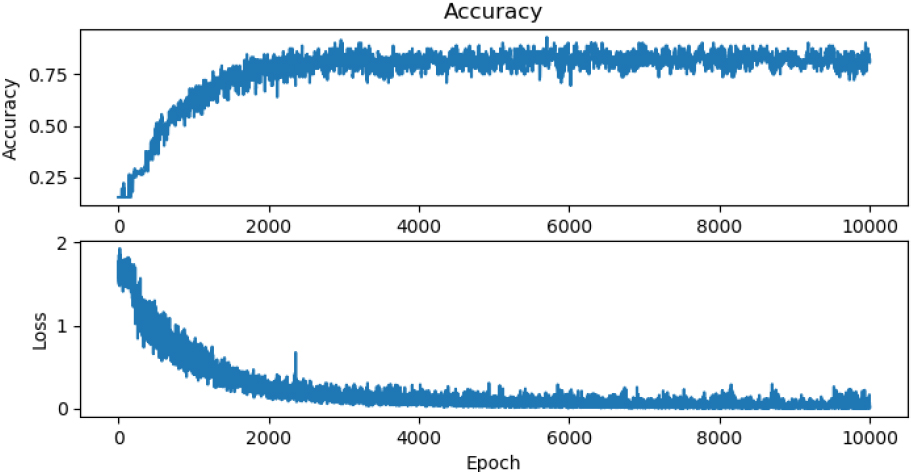
Figure 15.
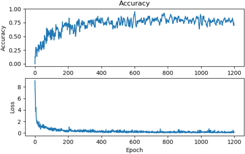
Accuracy and Loss performance measure experiment with pre-trained ResNet.
The VGG-3 network was trained on 1000 epochs with the learning rate set to 0.0005 and the accuracy of the network trained on this data was 0.875. The performance and shape of the curve are almost ideal (Fig. 13). This is because training results do not improve most of the time, and there are unnecessarily many epochs.
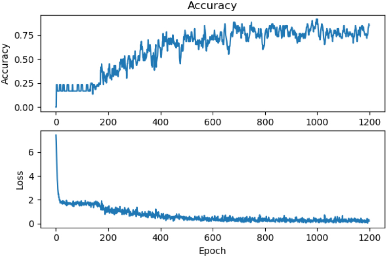
From Figs 13 and 14, it is observed that the training result does not improve from 1000 epochs to 10000 epochs. The same is observed from the VGG-4 network. Among the four networks, ResNet has the evolution of training on a pre-trained network. Initially, the accuracy of the training data rises faster than on the same network which it was not pre-trained. The difference in Accuracy and Loss performance measures on the pre-trained network and non-pre-trained ResNet can be observed in Figs 15 and 16.
This section describes the best-learned networks from each architecture and compares their results. The accuracy measurement on the categories is performed on a smaller dataset, so the accuracy sums do not correspond to the accuracy on the whole test dataset. The degree of rotation applied to the dataset is shown in Table 1. All values are given in degrees, and the individual values determine the category in the class.
5.3.1Performance evaluation on VGG-3
The best-measured network accuracy, which uses the VGG-3 architecture, on the test data was 97%.
Table 2
Predicting the class label on VGG-3 for different classes
| VGG-3 | Class_1 | Class_2 | Class_3 | Class_4 | Class_5 |
|---|---|---|---|---|---|
| Accuracy | 99% | 98% | 95% | 92% | 95% |
| Precision | 99% | 93% | 84% | 74% | 85% |
| Recall | 94% | 87% | 96% | 74% | 80% |
| F-measure | 97% | 90% | 89% | 74% | 82% |
Figure 16.
Accuracy and Loss performance measure experiment on non-pre-trained ResNet.
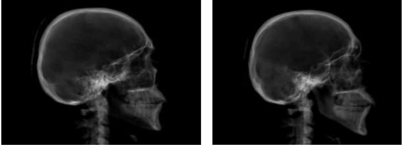
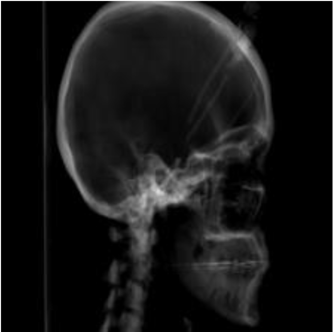
Here we can see from Table 2, the accuracy of the trained network in the individual classes, so it is clear that the network is confused in categories 3 and 4. These categories are interchanged. These categories are contiguous. So it’s not as serious a mistake as exchanging for a class at the opposite end in terms of rotation which will perform poorly on the VGG-3 network image. The misclassified image is shown in Fig. 17.
Table 3
Predicting the class label on VGG-4 for different classes
| VGG-4 | Class_1 | Class_2 | Class_3 | Class_4 | Class_5 |
|---|---|---|---|---|---|
| Accuracy | 99% | 98% | 94% | 93% | 98% |
| Precision | 99% | 93% | 78% | 84% | 89% |
| Recall | 94% | 87% | 95% | 68% | 94% |
| F-measure | 97% | 90% | 86% | 75% | 91% |
Table 4
Predicting the class label on Half-UNet for different classes
| Half-UNet | Class_1 | Class_2 | Class_3 | Class_4 | Class_5 |
|---|---|---|---|---|---|
| Accuracy | 88% | 85% | 68% | 91% | 98% |
| Precision | 99% | 10% | 38% | 65% | 99% |
| Recall | 25% | 0% | 85% | 72% | 78% |
| F-measure | 35% | 0% | 52% | 68% | 88% |
Figure 17.
A misclassified image of VGG3 networks.
5.3.2Performance evaluation on VGG-4
This network achieved an accuracy of 98% during testing. This is the best result that was achieved in experimenting on all implemented architectures.
From Table 3, as can be seen from this measurement of the VGG-4 network, the network was mainly involved in the first three categories, which are also confused and classified poorly on the VGG-4 network image. The misclassified image is shown in Fig. 18.
5.3.3Performance evaluation on Half-UNet
Half-UNet architecture achieves the worst of the architectures. Its accuracy on test data is 63%.
Table 4 shows that most of the misclassified images are from classes 1, 2, 3, 4, and 5. The Half-UNet network confuses these classes. These classes are right next to each other in head rotation and have the finest resolution that this network can’t handle very well. Not a single positive image was correctly assigned to the category. Therefore, it was not possible to calculate metrics such as recall and F-measure.
5.4Comparative analysis
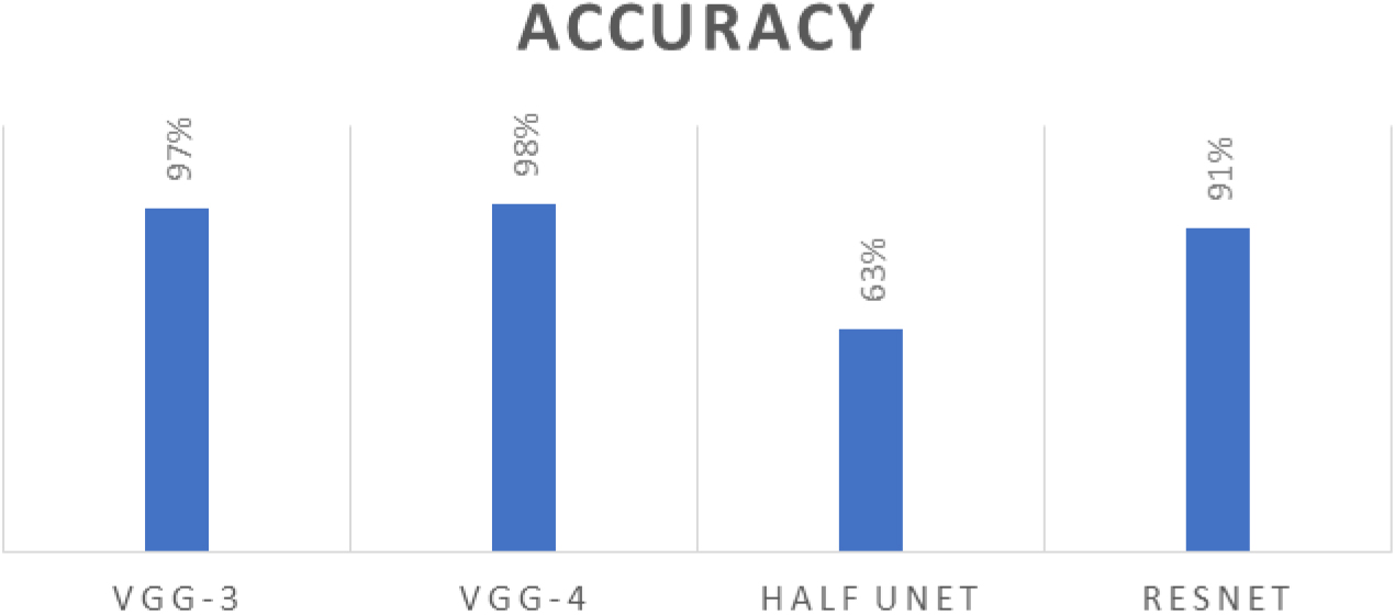
Figure 19, represents the Accuracy comparison among VGG-3, VGG-4, Half-UNet, and ResNet networks. The VGG-4 network attained high accuracy with VGG-3. On the contrary, the worst overall accuracy on the test data was the Half-UNet network architecture, which lags significantly behind all the others.
Table 5
Predicting the class label on ResNet for different classes
| ResNet | Class_1 | Class_2 | Class_3 | Class_4 | Class_5 |
|---|---|---|---|---|---|
| Accuracy | 96% | 94% | 98% | 99% | 99% |
| Precision | 81% | 81% | 94% | 99% | 99% |
| Recall | 90% | 81% | 94% | 90% | 99% |
| F-measure | 85% | 81% | 94% | 95% | 99% |
Figure 18.
A misclassified image of VGG3 networks.
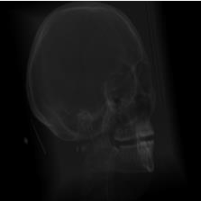
Figure 19.
Accuracy comparison among VGG-3, VGG-4, Half-UNet, ResNet networks.
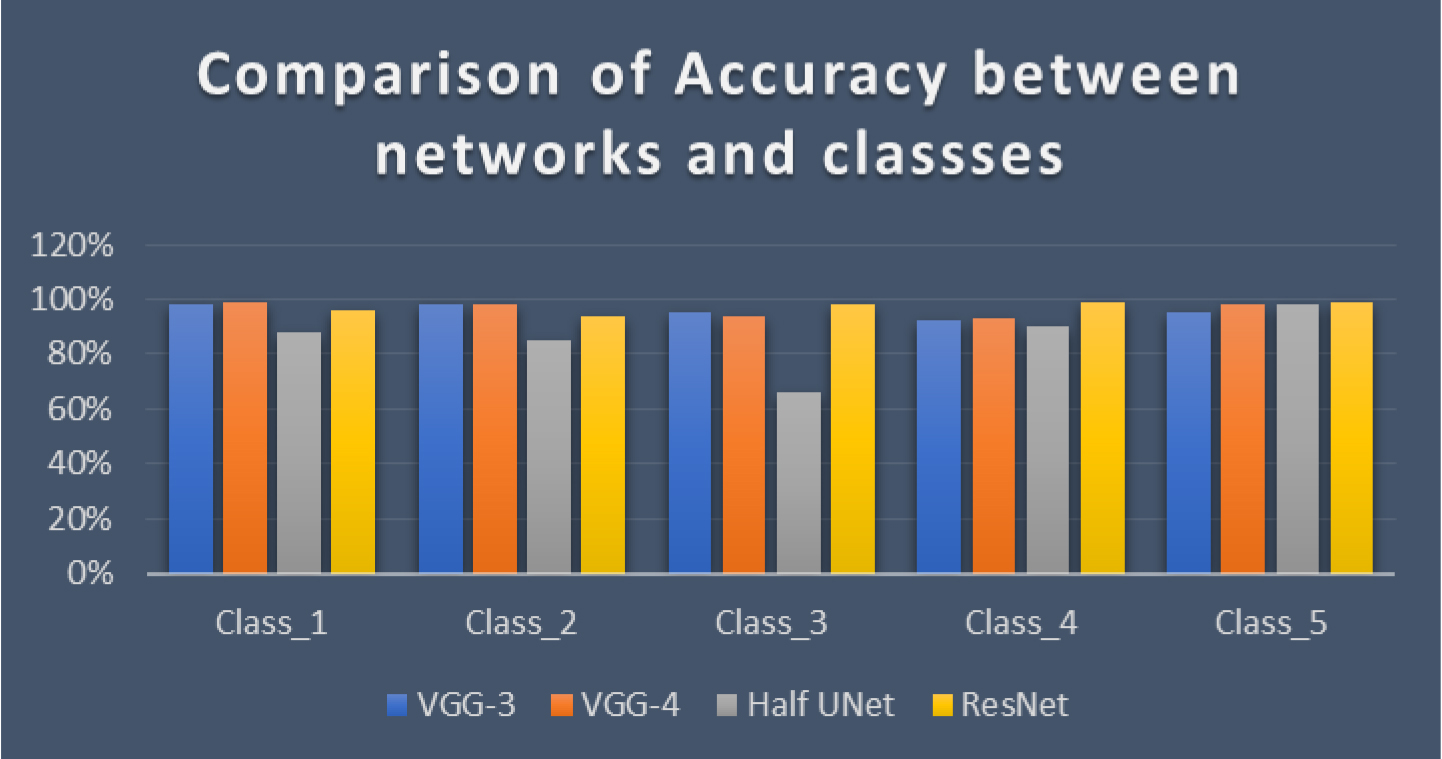
It is also interesting to compare the accuracy of individual classes between networks. The detailed comparison is shown in Table 6.
Table 6
Comparison of accuracy between networks and classes
| Accuracy | Class_1 | Class_2 | Class_3 | Class_4 | Class_5 |
|---|---|---|---|---|---|
| ResNet | 96% | 94% | 98% | 99% | 99% |
| Half-UNet | 88% | 85% | 66% | 90% | 98% |
| VGG-3 | 98% | 98% | 95% | 92% | 95% |
| VGG-4 | 99% | 98% | 94% | 93% | 98% |
Table 6 and Fig. 20 show that categories Class_2 and Class_4 are observed as the most difficult for analysis, where it confuses networks with category 3. In this area of rotation, there is a division into classes at smaller intervals. This means that the images in the different categories are very similar, leading to confusion. For example, the difference in rotation between categories can be one degree which can fall into error with slide annotations.
Table 7
Comparison of precision between networks and classes
| Precision | Class_1 | Class_2 | Class_3 | Class_4 | Class_5 |
|---|---|---|---|---|---|
| ResNet | 81% | 82% | 94% | 100% | 99% |
| Half-UNet | 99% | 10% | 38% | 69% | 100% |
| VGG-3 | 99% | 93% | 83% | 74% | 87% |
| VGG-4 | 99% | 93% | 78% | 84% | 89% |
The precision determines which accuracy will recognize positive pictures of the category. Table 7 elaborates on the comparison of precision between networks and classes In general; it is observed that the biggest problems have classes recognizing Class_3 and Class_4.
Table 8
Recall the comparison between networks and classes
| Recall | Class_1 | Class_2 | Class_3 | Class_4 | Class_5 |
|---|---|---|---|---|---|
| ResNet | 90% | 81% | 94% | 90% | 99% |
| Half-UNet | 21% | 18% | 85% | 72% | 78% |
| VGG-3 | 94% | 87% | 96% | 74% | 81% |
| VGG-4 | 93% | 87% | 95% | 68% | 94% |
Figure 20.
Comparison of Accuracy between networks and classes.
From this Table 8, it is clear that networks have the biggest problem with capturing images belonging to Class_2 and Class_4.
The F-measure corresponds to the findings from previous metrics. Table 9, represents the comparison of F-Measure between networks and classes. This is mainly because it is calculated as a combination of them. It gives us a more comprehensive view of network capabilities.
5.5Binary classifier
When the networks are used for analysis, it is important to realize whether the X-Ray image is suitable for Cephalometric analysis. From this point of view, the network results are only interested in how accurately the network places the images in class_3. This class corresponds to the image where the head is in the correct position. Therefore, it can interpret the results of the implemented networks as positive in the case of class_3 and negative for all others. In this way, a binary classifier simulation is created. Of course, this is only a simulation, so it is impossible to measure certain typical metrics. Table 10 and Fig. 21 will clarify further that most networks can also reliably solve this problem. The exception is Half-UNet, which has bigger problems with this resolution.
Table 9
Comparison of F-Measure between networks and classes
| F-measure | Class_1 | Class_2 | Class_3 | Class_4 | Class_5 |
|---|---|---|---|---|---|
| ResNet | 85% | 81% | 94% | 95% | 100% |
| Half-UNet | 45% | 24% | 52% | 68% | 88% |
| VGG-3 | 97% | 90% | 89% | 74% | 82% |
| VGG-4 | 97% | 90% | 87% | 75% | 91% |
Table 10
Comparison of metrics between networks on a Binary classifier
| Class_3 | Accuracy | Precision | Recall | F-measure |
|---|---|---|---|---|
| ResNet | 98% | 94% | 94% | 94% |
| Half-UNet | 67% | 56% | 86% | 80% |
| VGG-3 | 95% | 84% | 96% | 89% |
| VGG-4 | 94% | 78% | 95% | 86% |
Figure 21.
Comparison of metrics between networks on a Binary classifier.
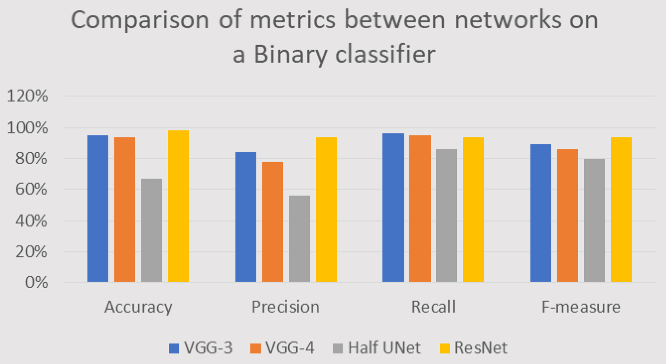
The VGG networks worked best, with only a minimal difference between them and the ResNet networks. The overall measured accuracy is 97% for VGG-3 and 98% for VGG-4. ResNet also has very good results (91%) for class_3 (
6.Conclusion
This paper aimed to predict the head position of an X-Ray image using Convolutional Neural Networks. The analysis takes place in such a way that it recognizes whether the image is suitable and, if not, suggests a change in the position of the head for correction. The recommendation for remediation is derived from the category in which the network image was included.
This paper addresses the exact rotation of the head position for Cephalometric analysis. The images were generated based on CT scans of the human head. The training has 1867 images in all categories, while the test dataset is 90 images. To achieve accurate prediction, the dataset was divided into 5 classes, with a degree of head rotation.
For this predicting head position for Cephalometric analysis, four networks are created in this experiment -two networks are of the VGG-Net type, one is UNet type, and the last is ResNet type. The U-Net-based network has been modified to meet the requirements of the prediction, and half of the original architecture has been removed called half-UNet. In the trained deep learning networks, the accuracy for each network that predicts the head position on the generated X-Ray image is evaluated. The accuracy of the head position prediction on VGG-3 is 97%, on VGG-4 it is 98%, and ResNet with an accuracy of 90%. The worst problem is solved by the Half-UNet network, which achieves an accuracy of only 61%. The results on Half-UNet could probably be improved by pre-training. It would also help if networks were trained on real data instead of artificially generated ones.
Another interesting direction that could be taken in further development is that it would directly calculate the angles of rotation of the head instead of just shifting into intervals. This could then be used in combination with my solution and increase the accuracy of the result. However, they evaluate the accuracy positively, since incorrectly classified images were classified directly adjacent to the correct ones at intervals.
References
[1] | A. Krizhevsky, I. Sutskever and G.E. Hinton, ImageNet Classification with Deep Convolutional Neural Networks, Springer Advances in Neural Information Processing System 25: ((2012) ), 1097–1105. |
[2] | A. Jiménez-Sánchez, D. Mateus, S. Kirchhoff, C. Kirchhoff, P. Biberthaler, N. Navab, M.A. González Ballester and G. Piella, Medical-based Deep Curriculum Learning for improved Fracture Classification, International Conference on Medical Image Computing and Computer Aided Interventions, MICCAI 2019, Lecture Notes in Computer Science, (2019) , p. 11769. |
[3] | A. Arévalo, J. Niño, G. Hernandez, J. Sandoval, D. León and A. Aragón, Algorithmic Trading Using Deep Neural Networks on High Frequency Data, Workshop on Engineering Applications ((2017) ), 144–155. |
[4] | C. Lindner, C.-W. Wang, C.-T. Huang, C.-H. Li, S.-W. Chang and T.F. Cootes, Fully Automatic System for Accurate Localisation and Analysis of Cephalometric Landmarks in Lateral Cephalograms, Scientific Reports Scientific Reports 1: (3) ((2016) ), 1–10. |
[5] | F. Schwendicke, A. Chaurasia, L. Arsiwala, J.-H. Lee, K. Elhennawy, P.-G. Jost-Brinkmann, F. Demarco and J. Krois, Deep Learning for Cephalometric Landmark Detection: Systematic Review and Meta-Analysis, Clinical Oral Investigations 7: (25) ((2021) ), 4299–4309. |
[6] | G. Li, H. Xie, H. Ning, D. Citrin, J. Capala, R. Maass-Moreno, P. Guion, B. Arora, N. Coleman, K. Camphausen and R.W. Miller, Accuracy of 3D Volumetric Image Registration Based on CT, MR, and PET/CT phantom experiments, Journal of Applied Clinical Medical Physics 4: (9) ((2008) ), 17–36. |
[7] | H.A. Al-Barazanchi and H. Qassim, A. Verma: Residual CNDS 2016, p. 8. |
[8] | H. Seo, C. Huang, M. Bassenne, R. Xiao and L. Xing, Modified U-Net (mU-Net) with Incorporation of Object-Dependent High-Level Features for Improved Liver and Liver-Tumor Segmentation in CT Images, IEEE Transactions on Medical Imaging 5: (39) ((2020) ), 1316–1325. |
[9] | K. He, X. Zhang, S. Ren and J. Sun, Deep Residual Learning for Image Recognition, (2015) . |
[10] | K. Simonyan and A. Zisserman, Very Deep Convolutional Networks for Large-Scale Image Recognition, (2014) . |
[11] | L. Balagourouchetty, J.K. Pragatheeswaran, B. Pottakkat and R. G, GoogLeNet-Based Ensemble FCNet Classifier for Focal Liver Lesion Diagnosis, IEEE Journal of Biomedical and Health Informatics 24: (3) ((2020) ), 1686–1694. |
[12] | M. Levoy, Display of surfaces from volume data, IEEE Computer Graphics and Applications 3: (8) ((1988) ), 29–37. |
[13] | M. Sakamoto and H. Nakano, Cascaded Neural Networks with Selective Classifiers and its Evaluation using Lung X-Ray CT Images, (2016) . |
[14] | M.S. Sorower, A Literature Survey on Algorithms for Multi-Label Learning, (2010) . |
[15] | M. Puttagunta and S. Ravi, Medical Image Analysis based on Deep Learning Approach, Multimedia Tools and Applications 80: ((2021) ), 24365–24398. |
[16] | National Institute of Health, https://openi.nlm.nih.gov/index.php. |
[17] | O. Ronneberger, P. Fischer and T. Brox, U-Net: Convolutional Networks for Biomedical Image Segmentation, In: Navab N, Hornegger J, Wells W, Frangi A. (eds) Medical Image Computing and Computer-Assisted Intervention – MICCAI 2015. Lecture Notes in Computer Science, (2015) , p. 9351. |
[18] | P.S.L. Maschtakow, J.L.O. Tanaka, J.C. da Rocha, L.C. Giannas, M.E.L. de Moraes, C.B. Costa, J.C.M. Castilho and L.C. de Moraes, Cephalometric analysis for the diagnosis of sleep apnea: a comparative study between reference values and measurements obtained for Brazilian subjects, Dental Press Journal of Orthodontics 3: (18) ((2013) ), 143–149. |
[19] | Python library to use the REST interface of the Virtual Skeleton Database https://github.com/SICASFoundation/vsdConnect. |
[20] | S. Rashmi, P. Murthy, V. Ashok and S. Srinath, Cephalometric Skeletal Structure Classification Using Convolutional Neural Networks and Heatmap Regression, SN Computer Science 5: (3) ((2022) ). |
[21] | S. Ioffe and C. Szegedy, Batch Normalization: Accelerating Deep Network Training by Reducing Internal Covariate Shift, (2015) . |
[22] | J. Škandera, Landmark Detection in medical images using deep neural networks. Ph.D. Dissertation, Brno University of Technology, (2019) . |
[23] | The SICAS Medical Image Repository, https://www.smir.ch/. |
[24] | X. Li, H. Chen, X. Qi, Q. Dou, C-W. Fu and P.A. Heng, H-DenseUNet: Hybrid Densely Connected UNet for Liver and Tumor Segmentation from CT Volumes, IEEE Transactions on Medical Imaging 12: (37) ((2018) ), 2663–2674. |
[25] | Y.L. Thian, Y. Li, P. Jagmohan, D. Sia, V.E.Y. Chan and R.T. Tan, Convolutional neural networks for automated fracture detection and localization on wrist radiographs, Radiology: Artificial Intelligence 1: (1), (2019) . |
[26] | Y. Song, X. Qiao, Y. Iwamoto and Y.-W. Chen, Automatic Cephalometric Landmark Detection on X-ray Images Using a Deep-Learning Method, Applied Sciences 7: (10) ((2020) ), 2547. |


