
Supervised probabilistic latent semantic analysis with applications to controversy analysis of legislative bills
Abstract
Probabilistic Latent Semantic Analysis (PLSA) is a fundamental text analysis technique that models each word in a document as a sample from a mixture of topics. PLSA is the precursor of probabilistic topic models including Latent Dirichlet Allocation (LDA). PLSA, LDA and their numerous extensions have been successfully applied to many text mining and retrieval tasks. One important extension of LDA is supervised LDA (sLDA), which distinguishes itself from most topic models in that it is supervised. However, to the best of our knowledge, no prior work extends PLSA in a similar manner sLDA extends LDA by jointly modeling the contents and the responses of documents. In this paper, we propose supervised PLSA (sPLSA) which can efficiently infer latent topics and their factorized response values from the contents and the responses of documents. The major challenge lies in estimating a document’s topic distribution which is a constrained probability that is dictated by both the content and the response of the document. To tackle this challenge, we introduce an auxiliary variable to transform the constrained optimization problem to an unconstrained optimization problem. This allows us to derive an efficient Expectation and Maximization (EM) algorithm for parameter estimation. Compared to sLDA, sPLSA converges much faster and requires less hyperparameter tuning, while performing similarly on topic modeling and better in response factorization. This makes sPLSA an appealing choice for latent response analysis such as ranking latent topics by their factorized response values. We apply the proposed sPLSA model to analyze the controversy of bills from the United States Congress. We demonstrate the effectiveness of our model by identifying contentious legislative issues.
1.Introduction
Hofmann [1] introduced Probabilistic Latent Semantic Analysis (PLSA), which is also known as Probabilistic Latent Semantic Indexing (PLSI) when used in information retrieval and text mining [2]. The basic idea of PLSA is to treat the words in each document as observations from a mixture model where the components of the model are word distributions for latent topics. The selection of the latent topics is controlled by a set of mixing weights such that words in the same document share the same mixing weights. PLSA was initially proposed for text-based applications that do indexing, retrieval, mining, and clustering. Later, its use was expanded to other fields including collaborative filtering [3], computer vision [4], and audio processing [5].
PLSA can be viewed as a probabilistic version of the seminal work on latent semantic analysis [6], which revealed the utility of the singular value decomposition of the document-term matrix. PLSA is the precursor of probabilistic topic models which are widely used nowadays including Latent Dirichlet Allocation (LDA) [7]. The basic generative processes of PLSA and LDA are very similar. In PLSA, the topic mixture is conditioned on each document, while the topic mixture in LDA is drawn from a conjugate Dirichlet prior. Theoretically, PLSA is equivalent to MAP estimated LDA under a uniform prior [8]. The PLSA model does not make any assumptions about how the mixture weights are generated and thus its generative semantics are not well defined [7]. Consequently, there is no natural way to predict a previously unseen document. On the other hand, the LDA model is more complex and cannot be solved by exact inference. Gibbs sampling [9] and variational inference [7] are often used for inference in LDA type of topic models. However, these methods scale poorly to large datasets. Variational inference requires dozens of expensive passes over the entire dataset, and Gibbs sampling requires multiple Markov chains [10]. In contrast, the parameter estimation and inference of PLSA can be efficiently done by the EM algorithm.
PLSA and LDA are the two most representative topic models. Various empirical comparisons have been conducted between them. Blei et al. [7] shows that LDA outperforms PLSA in the perplexity of new documents. On the other hand, Lu et al. [11] conduct a systematic empirical study of PLSA and LDA on three representative IR tasks, including document clustering, text categorization, and ad-hoc retrieval. They found that LDA and PLSA tend to perform similarly on these tasks. Furthermore, the performance of LDA on all tasks is quite sensitive to the setting of its hyperparameters, and the optimal setting of hyperparameters varies according to how the model is used in a task.
The original PLSA and LDA models as well as most of their variants are unsupervised models. Many real-world text documents are associated with a response variable connected to each document such as the number of stars given to a movie, the number of times a news article was downloaded, or the category of a document. Incorporating such information into latent aspect modeling could guide a topic model towards discovering semantically more salient statistical patterns that may be more interesting or relevant to the user’s task. Thus, a very important extension of LDA is supervised LDA (sLDA) [12]. sLDA jointly models the content and responses of documents in order to find latent topics that best predict the responses of documents.
In this paper, we propose supervised Probabilistic Latent Semantic Analysis (sPLSA) by extending PLSA to learn from the responses of documents. For PLSA, our proposed model is the analog of what sLDA is to LDA. The major challenge lies in estimating a document’s topic distribution which is a constrained probability that is dictated by both the content and the response of the document. We introduce an auxiliary variable to transform the constrained optimization problem to an unconstrained optimization problem. This allows us to derive an efficient EM algorithm to estimate the parameters of our model. Compared to sLDA, sPLSA is much more efficient and requires less hyperparameter tuning, while performing similarly on topic modeling and better in response factorization. This makes sPLSA the ideal choice for latent response analysis such as ranking latent topics by their factorized response values. We utilize the sPLSA model to analyze the controversy of bills from the United States Congress. We demonstrate the effectiveness of our model by identifying contentious legislative issues. The contributions of the paper can be summarized as follows.
• We propose a novel supervised PLSA model which can efficiently infer latent topics and their factorized response values from the contents and the responses of documents.
• We derive an efficient EM algorithm to estimate the parameters of the model.
• We utilize sPLSA and sLDA to analyze the controversy of bills from the United States Congress. We demonstrate the effectiveness of sPLSA over sLDA as part of this analysis.
2.Related work
2.1Probabilistic topic models
In 1999, three papers [1, 2, 13] introduced the model of Probabilistic Latent Semantic Analysis. One variant of the model appeared in 1998 [14] and all these models were originally discussed in an earlier technical report [15]. PLSA was a probabilistic implementation of latent semantic analysis (LSA) introduced by Deerwester et al. [6]. LSA was extended from the vector space model. It aimed to represent documents in a low dimensional vector space consisting of common semantic factors. Differing from LSA in projecting document or word vectors into the latent semantic space, PLSA extracted the aspects related to documents. This aspect model was interpreted as a mixture model containing latent semantic mixtures. Parameters of mixture probabilities were estimated by the maximum-likelihood (ML) principle. PLSA did not provide a straightforward way to make inferences about new documents not seen in the training data and the parameterization of the model was susceptible to overfitting. Latent Dirichlet Allocation (LDA) addressed these limitations by proposing a Bayesian probabilistic topic model.
PLSA and LDA established the field of probabilistic topic models. Many extensions of the two basic models have been proposed. In Zhai et al. [16], PLSA was extended to include a background component to explain the non-informative background words and a cross-collection mixture model was proposed to support comparative text mining. Mei and Zhai [17] propose a general contextual text mining model which is an extension of PLSA to incorporate context information. They further regularize PLSA with a harmonic regularizer based on a graph structure in the data [18]. One active area of topic modeling research is how to relax and extend the assumptions of PLSA and LDA to uncover more sophisticated structure in the texts. For example, the work by Rosen-Zvi et al. [19] extends LDA to include authorship information. Recently, probabilistic topic models are proposed for unsupervised many-to-many object matching [20] and cross-lingual tasks [21]. There are many other topic models proposed. Blei [22] gives an overview of the field of probabilistic topic models.
The original PLSA and LDA and most of their variants are unsupervised models. Blei and McAuliffe [12] proposed supervised LDA (sLDA) to capture real-valued document rating as a regression response. The generative process of sLDA is similar to LDA, but with an additional step: draw a reponse variable. The sLDA model is trained by maximizing the joint likelihood of the contents and the responses of documents. They tested sLDA on two real-world datasets: movie reviews with ratings and web pages with popularity, and the experimental results demonstrated the advantages of sLDA versus regularized regression, and versus an unsupervised LDA analysis followed by a separate regression. Other extensions include multi-class sLDA [23], which directly captures discrete labels of documents as a classification response; and discriminative LDA (DiscLDA) [24], which also performs classification, but with a mechanism different from that of sLDA; and MedLDA [25], which leverages the maximum margin principle for estimation of latent topical representations. Recently, Jameel et al. [26] integrate class label information and word order structure into a supervised topic model for document classification. More variants of supervised topic models can be found in a number of applied domains, such as Labeled LDA [27], automatic summarization of changes in dynamic text collections [28], modeling of numerical time series [29], inferring topic hierarchies [30], and query expansion [31]. In computer vision, several supervised topic models have been designed for understanding complex scene images [32, 33]. Mimno and McCallum [34] also proposed a topic model for considering document-level meta-data; for example, publication date and venue of a paper.
Most of the above supervised topic models are based on LDA. There exist very few work on extending PLSA to the supervised setting. One such work was to use the spoken content of a multimedia document as a query for retrieving similar or relevant documents [35]. The query was used to train the model in a supervised fashion with respect to a query-document similarity objective function. Fergus et al. [36] extend PLSA to include spatial information in a translation and scale invariant manner, and utilized this modified PLSA model to learn an object category. Another work added a category-topic distribution in PLSA for human action recognition [37]. However, these models do not associate the topic distribution of the document with the response variable. Consequently, the discovered topics may not be indicative of the response. Aliyanto et al. [38] proposed a version of supervised PLSA to estimating technology readiness level, but they assumed the topics of each word in a document are observed which are actually not available in many real-world applications. In this paper, we follow the way LDA was extended to sLDA by directly associating the documents’ topic distributions with the response. The response is at the document level instead of the word level and it is more readily accessible. The learned topics depend on both the document’s content and response. To the best of our knowledge, no prior work has extended PLSA in a similar manner.
Recently, with the rise of deep learning, novel topic models based on neural networks have been proposed. Salakhutdinov and Hinton [39] proposed a two layer restricted Boltzmann machine (RBM) called the replicated-softmax to extract low level latent topics from a large collection of unstructured documents. Larochelle and Lauly [40] proposed a neural auto-regressive topic model inspired from the replicated softmax model but replacing the RBM model with a neural auto-regressive distribution estimator (NADE). Kingma and Welling [41] proposed variational autoencoders by combining topic modeling and neural networks. Cao et al. [42] proposed neural topic model (NTM), and it is supervised extension (sNTM) where words and documents embedding are combined. Moody [43] proposed the lda2vec, a model combining LDA and word embeddings. Dieng et al. [44] integrated to a recurrent neural network based language model global word semantic information extracted using a probabilistic topic model. Gupta et al. [45] integrated to an LSTM recurrent neural network, a neural auto-regressive topic model. Murakami and Chakraborty [46] investigated the use of word embedding with NTM for interpretable topics from short texts. Grootendorst [47] proposed BERTopic to generate document embedding with pre-trained transformer-based language models and then produce topic representations with the class-based TF-IDF procedure. Two recent surveys [48, 49] provided comprehensive reviews of neural topic models, with nearly a hundred models developed and a wide range of applications in neural language understanding such as text generation, summarization and language models. Despite the popularity of deep learning, our work has focused on traditional probabilistic methods because they are often easier to implement and more efficient to train, which may be more suitable in resource constrained environments where only limited computation and storage are accessible. Nevertheless we will explore to combine the proposed model with neural networks in a future work.
2.2Controversy analysis of legislative bills
Legislative voting is a major area of research. Most of the research is focused on the ideal point estimation of the ideological positions of legislators. This is primarily for the purpose of predicting their voting patterns. An early work in this area presented a spatial model of legislative voting [50]. Londregan [51] estimated the preferred positions of legislators by modeling the legislative agenda. Cox and Poole [52] used a spatial model to assess the role of partisanship in influencing the votes of legislators. Variational methods were applied to predict votes [53]. Thomas et al. [54] modeled voting behavior from congressional debate transcripts. Gerrish and Blei [55] demonstrated roll call predictive models which link legislative text with legislative sentiment. They [56] further derived approximate posterior inference algorithms based on variational methods to predict the positions of legislators. Fang et al. [57] analyzed public statements from legislators to build a contrastive opinion model of the legislators. Gu et al. [58] conducted ideal point estimations of legislators on the latent topics of voted documents.
Some of the work cited above utilized topic models. For example, Gerrish and Blei [55] extended LDA to build a generative model of votes and bills called the ideal point topic model. The model infers two bill related latent variables. One of the latent variables explains bills that all legislators will vote for or against while the other variable explains bills that do not have unanimous approval or disapproval. In addition, the model infers a latent variable for the legislators’ ideal points. Another example, Fang et al. [57] present the cross-perspective topic model which unifies two identically extended LDA models to contrast the opinion words of a bipolar legislative body. The opinion words reflect the subjective positions of the polar entities on various topics. The model discriminates between opinion words and topics words by treating them as two separate observed variables.
On the broader field of controversy analysis, much work has been done detecting contradictions in textual data. One of the early works studied the dynamics of conflicting opinions in texts by visually inspecting graphs [59]. Tsytsarau et al. [60] further investigated two types of contradictions, namely, “overlapping contradicting opinions” and “change of sentiment”. Many supervised learning approaches have been proposed for classifying texts into one of the two opposing opinions using annotated controversial corpora including sentences [61], documents [62] and document collections [61]. Some recent work addresses the task of identifying controversial contents on Wikipedia [63, 64, 65] and on social media [66, 67, 68].
Table 1
Notations
|
| Corpus of documents |
| A document in |
|
| A word that occurs in |
| A topic |
|
| Count of word |
| Total number of topics |
|
| Total number of words |
| Number of words in |
|
| Total number of documents |
|
|
|
| Topic distribution of |
| Matrix of all |
|
|
|
| Word distribution of |
|
| Matrix of all |
| Topic of the |
|
|
| Matrix of all | |
|
| Response of |
| Vector of all |
|
| Regression coefficient on topic |
| Vector of all |
|
| Variance of the Gaussian noise |
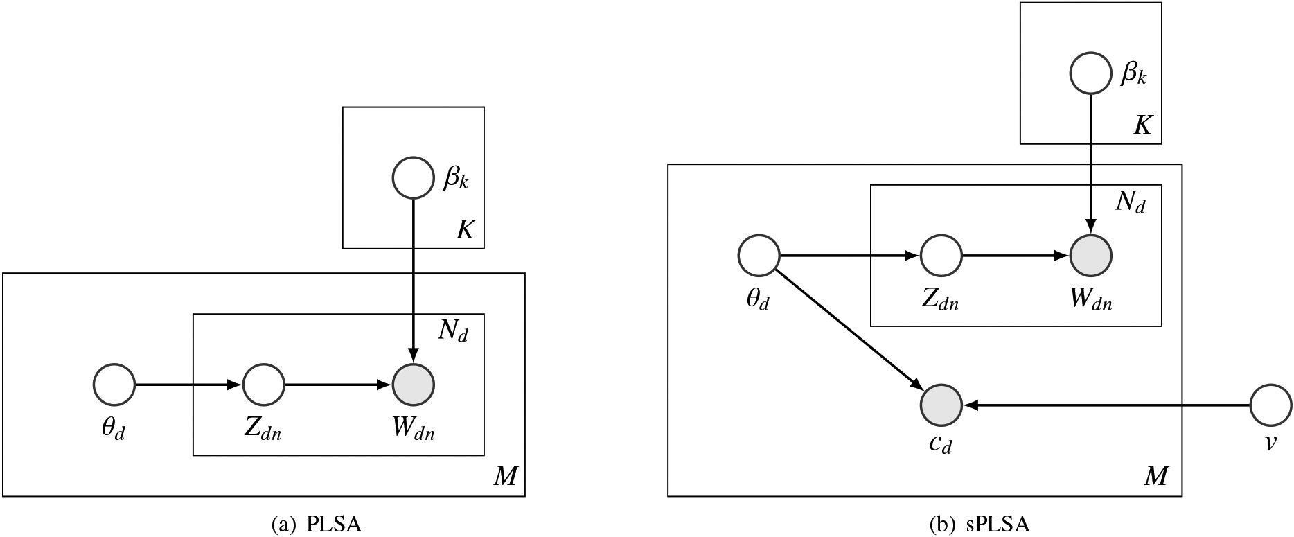
Figure 1.
Graphical model representation of (a) PLSA and (b) sPLSA.
3.Supervised PLSA
3.1Notations
Assume the corpus
3.2Generative process
Similar to many other topic models, sPLSA assumes that a document consists of multiple topics. Therefore, there is a distribution
The essential difference between PLSA and sPLSA lies in the modeling of the response variable
• For each word
– Choose a topic
– Choose a word
• Draw a response
Here the response comes from a Gaussian linear model. The mean is the inner product of topic distribution
Figure 1 illustrates the graphical model representation of PLSA and sPLSA, respectively.
It is worth noting that our approach for modeling
3.3Likelihood function
The likelihood function in supervised PLSA consists of two parts. The first part is the likelihood for observing all the words in the corpus,
(1)
where
(2)
The second part of the likelihood function comes from the likelihood of the response variable. As shown in the generative process, we assume a linear model with Gaussian noise for modeling the response
(3)
where
(4)
where
We assume a Gaussian prior on the coefficients
(5)
Equations (2) and (5) share
(6)
where
3.4Parameter estimation
Now that we have established the unified likelihood, we can use it to derive formulas for iteratively updating the parameters
Figure 2.
The iterative updates of the parameter estimation process.
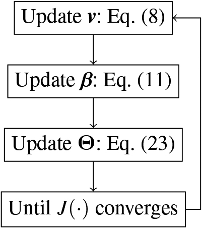
3.4.1Updating 𝐯
The values of
(7)
It can be seen that the above objective function is strictly convex in
(8)
This solution is equivalent to Ridge Regression or Tikhonov regularization [69].
3.4.2Updating β
The values of
(9)
In the M-step, we maximize the expected complete data log-likelihood as follows:
(10)
with the constraint of
(11)
3.4.3Updating 𝚯
The values of
(12)
Since the second and third terms in the above lower bound are constants with respect to
(13)
This means we use the following objective instead of the unified likelihood to update
(14)
The above objective is a concave function with respect to
(15)
The constraint must be met because each
(16)
where
(17)
Irrespective of the value of
Furthermore, we can reduce the number of
(18)
when
(19)
As a result, we can express
(20)
This results in
(21)
and to the following when
(22)
Finally, we can express
(23)
The above representation of
We use the gradient ascent algorithm to maximize the objective function
(24)
where:
(25)
and:
(26)
After we update each
3.5Inference
After the parameter estimation is completed, we do the following to infer the latent topics and their factorized response values:
• We infer the latent topics from the topic-word distribution
• We infer the factorized response for each latent topic
4.Experiments
In this section, we discuss the dataset we used to test sPLSA, present experimental results, and compare our model to the baselines.11
4.1Dataset
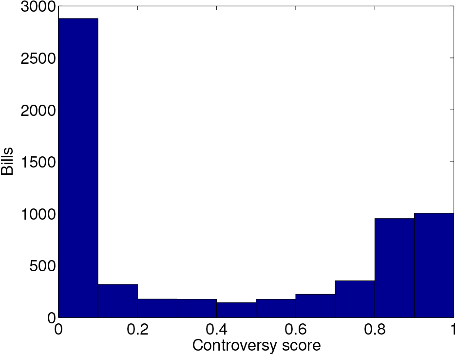
We tested sPLSA using bills which were placed for a vote in the United States Congress. The objective of our test is to generate the latent topics of the bills, and then rank them by controversy. We do this by first assigning a controversy score to each bill followed by inferring the factorized controversy score of each topic using sPLSA. We assign a controversy score to each bill by using the spread of the number of yes and no votes. The formula we use is as follows:
(27)
where
The reason why we selected congressional bills and their controversy scores as our dataset is to demonstrate applying sPLSA to a real world problem. Specifically, we want to identify contentious issues in the United States Congress by generating their latent topics. By inferring their relative controversy using sPLSA, we can rank the topics by controversy, and identify the contentious issues by selecting the most controversial topics.
We collected bills starting from the
We were able to collect the votes and content of 6,403 bills. 5,531 bills were from the House of Representatives and 872 bills were from the Senate. 6,160 bills had more yes votes than no votes, and 243 bills had more no votes than yes votes. Figure 3 shows the distribution of the bills’ controversy score.
We did the following preprocessing of the bills to create our dataset:
• Removed words which have characters that are not in the English alphabet.
• Removed words less than 4 characters in length.
• Removed common English words using Mallet’s44 stop-word list.
• Removed domain specific words using a custom stop-word list. The stop-word list has 157 words, and we created it by analyzing the word frequency of the bills. It mostly consists of legal terms.
• Selected the 15,000 most frequent words as the vocabulary of our corpus.
We then created the dataset as a bag-of-words representation of each bill.
4.2Setup
We randomly partition our dataset as follows: 80% for training, 10% for validation, and 10% for testing. We initialize
4.3Evaluation metrics
We test a trained model by folding-in the test dataset similar to the way specified in [1]. This is essentially the same as training the model with the test dataset except
• For
• For
(28)
The higher the correlation between
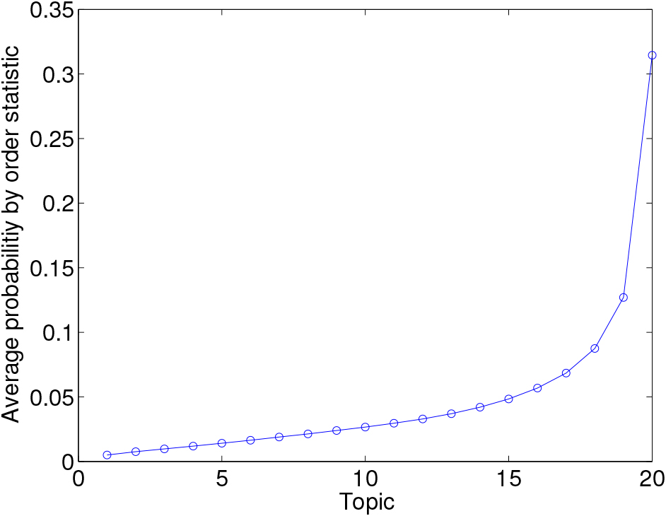
The reason why we can correlate each
Figure 4.
The sparsity of
4.4Results
Table 2 shows the top 5 words for the
Table 2
The top 5 words for the
| Rank |
|
|
|
|
|---|---|---|---|---|
| 1 |
|
|
|
|
| Fundraising | Fisa | Alien | Educating | |
| Expense | Buddhist | Immigrants | Institutes | |
| Fisa | Outdoor | Secures | High | |
| Alien | Functions | Employing | Struggle | |
| Secures | Loaded | Stationing | Structuring | |
| 2 |
|
|
|
|
| Fundraising | Fundraising | Fisa | Payers | |
| Fisa | Expense | Buddhist | Fisa | |
| Buddhist | Relocates | Expense | Indispensable | |
| Expense | Appropriations | Fundraising | Paygo | |
| Appropriations | Expendable | Functions | Plain | |
|
|
|
|
|
|
| Defending | Finances | Foregone | Education | |
| Milestone | Commissary | Internal | Schofield | |
| Fisa | Board | Secures | Lobbying | |
| Forced | Persian | Nation | Educating | |
| Forbs | Companionship | Verifying | Childless | |
|
|
|
|
|
|
| Plain | Propene | Defending | Chances | |
| Propene | Therapeutics | Milestone | Header | |
| Lancaster | Chaplains | Proclaimed | Chaplains | |
| Mammography | Lien | Forbs | Sequester | |
| Tarp | Fisa | Researcher | Frederick | |
|
|
|
|
|
|
| Healing | Drowning | Commissary | Houses | |
| Houses | Prison | Safeguarding | Expense | |
| Fundraising | Bushel | Chaplains | Prohibited | |
| Secures | Mammography | Vessel | Amounts | |
| Payers | Sttr | Transnational | Distributors |
4.4.1Comparison to baseline
Our baseline is an sLDA model. The response variable for the model is the controversy score. We used the ’slda.em’ function in the R “lda” package55 to train the sLDA model using the training dataset. We run the model for each
Table 3
Comparison of the Pearson correlation between
|
| 10 | 20 | 30 | 40 |
|---|---|---|---|---|
| sPLSA | 0.9837 | 0.9850 | 0.9632 | 0.9182 |
| sLDA | 0.9530 | 0.8427 | 0.7550 | 0.4614 |
sPLSA is designed for topic discovery and latent response inference. This comes at the expense of its prediction performance. Theoretically, we can use sPLSA in a semi-supervised setting where we mix both labeled and unlabeled data, and then try to predict the labels for the unlabeled data. In such a scenario, we update
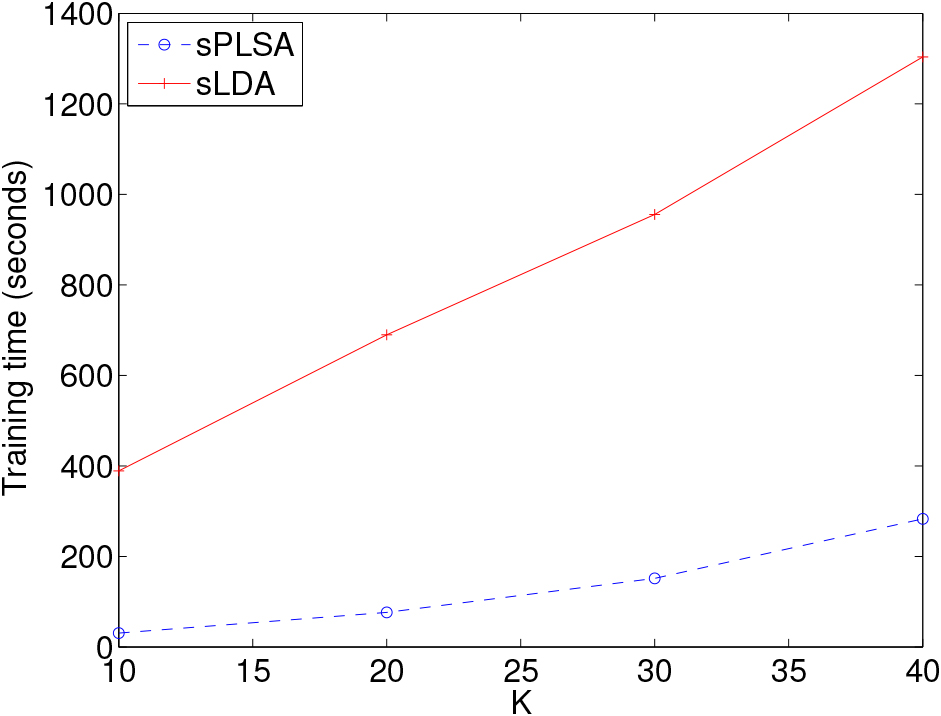
4.4.2Efficiency
We run sPLSA and sLDA on a MacPro laptop with a 2 GHz processor and 16 GB RAM on the training dataset for various values of
The reason why Gibbs sampling converges a lot slower than the EM algorithm is because the topics tend to depend on one another. This prolongs the burn-in period for the Gibbs sampling process where a stationary distribution has not been achieved. A stationary distribution needs to be achieved for the actual sampling to take place. During the burn-in period, the Gibbs sampling process can diverge at times. On the other hand, EM does not have the equivalent of a burn-in period and every iteration of the algorithm is guaranteed to monotonically improve the convergence of the likelihood.
4.4.3Impact of η
We trained the model with
Table 4
The perplexity and Pearson correlation values on the validation dataset for different values of
|
| 0.001 | 0.01 | 0.1 | 1 | 10 | 100 | 1000 |
|---|---|---|---|---|---|---|---|
| Perplexity | 2072.6 | 2307.3 | 2062.4 | 2102.3 | 2056.7 | 2151.2 | 2053.5 |
| Correlation | 0.335 | 0.982 | 0.987 | 0.951 | 0.966 | 0.976 |
Figure 5.
The prediction RMSE values of sPLSA and sLDA at various values of
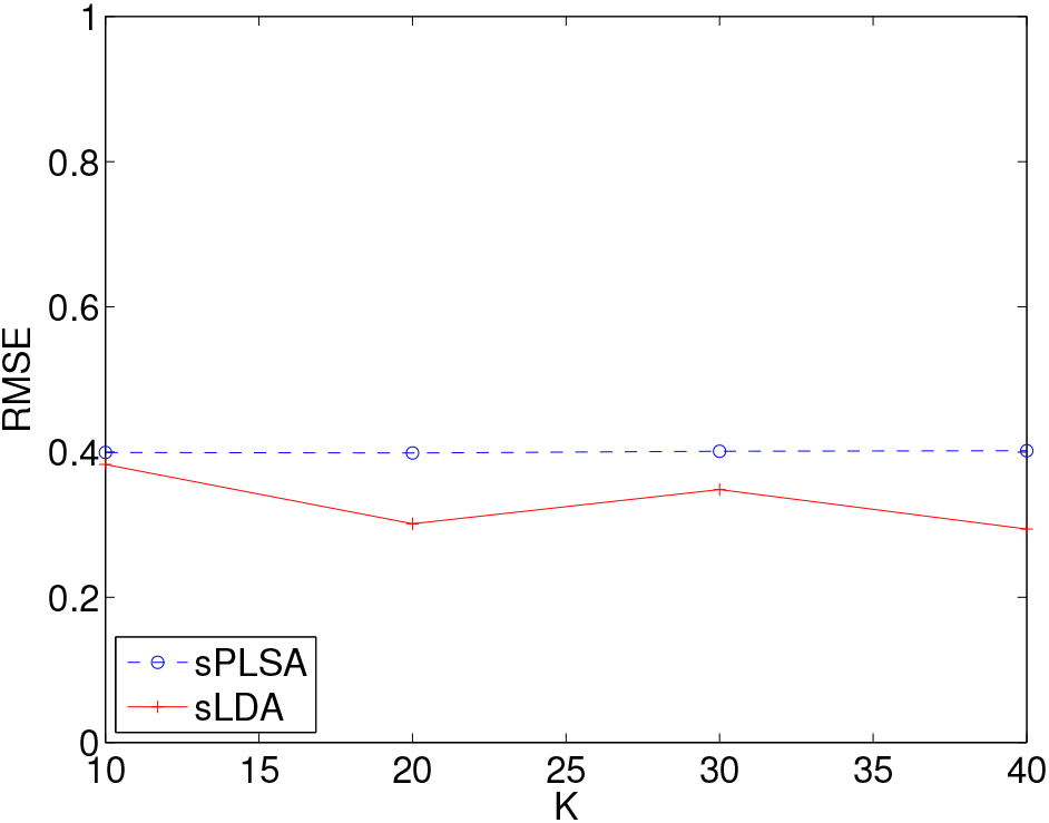
Figure 6.
Comparison of the training time of sPLSA and sLDA for various values of
4.4.4Impact of λ
We trained the model for each combination of
Figure 7.
The perplexity for various combinations of
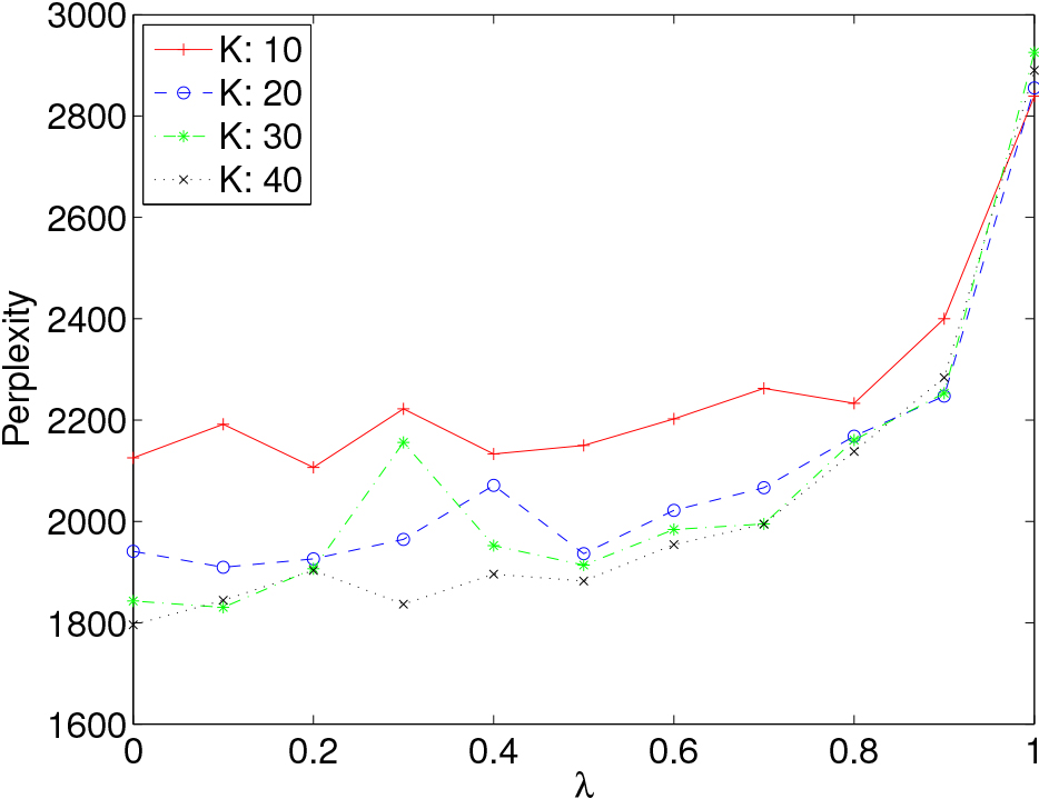
From the figure, we can generally see that as
Figure 8 shows the values of the Pearson correlation between
Figure 8.
The Pearson correlation between
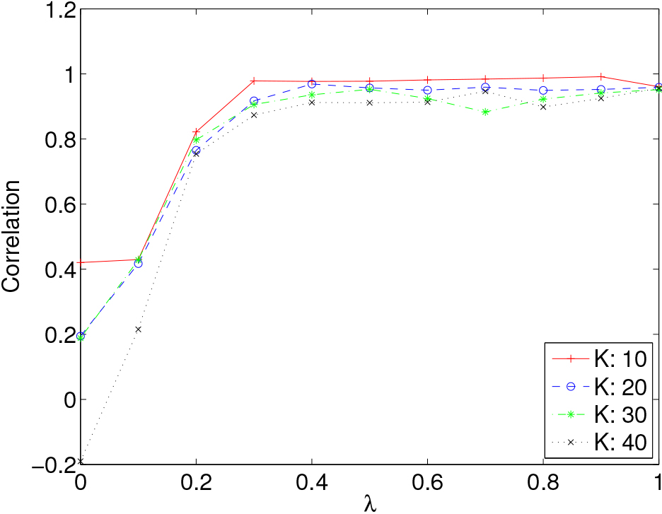
From the figure, we can generally see that the correlation increases steeply from
4.4.5Sample topics
Tables 5, 6, and 7 show the top words for the topics generated by PLSA, sLDA, and sPLSA. In general, we can see that very similar topics are generated by all three models. For example, topic 7 for PLSA, topic 2 for sLDA, and topic 6 for sPLSA are about education. This illustrates that the perplexity trade-off we did in selecting
Table 5
Top 5 words for the topics of PLSA when
| 1 | Transnational | Alien | Finances | Board | Persian |
|---|---|---|---|---|---|
| 2 | Fisa | Buddhist | Outdoor | Loaded | Healing |
| 3 | Washoe | Prohibited | Enemy | Lancaster | Mammography |
| 4 | Healing | Plain | Indispensable | Cards | Chiefs |
| 5 | Defending | Milestone | Fisa | Forbs | Forced |
| 6 | Plain | Houses | Inclusive | Indispensable | Propene |
| 7 | Education | Educating | Lobbying | Schofield | Fundraising |
| 8 | Secures | Intell | Directly | Foregone | Rescind |
| 9 | Fundraising | Expense | Appropriations | Fisa | Relocates |
| 10 | Defending | Fisa | Fundraising | Milestone | Plain |
Table 6
Top 5 words for the topics of sLDA when
| 1 | Foregone | Internally | Securitization | Nationally | Countries |
|---|---|---|---|---|---|
| 2 | Educating | Education | Lobbyists | Scholars | Childless |
| 3 | Fundraising | Blvd | Subsystem | Administrator | Entitles |
| 4 | Lance | Wastewater | Enemy | Conservancy | Prohibition |
| 5 | Defending | Milford | Forbs | Forced | Armstrong |
| 6 | Authorities | Constructing | Traineeships | Subsystem | Systematically |
| 7 | Plains | Healing | Paying | Cards | Inclusive |
| 8 | Persistent | Commissary | Coursework | Finances | Attitudes |
| 9 | Fundraising | Expense | Relocations | Transplantation | Appropriation |
| 10 | Fisa | Buddhist | Fundraising | Reseller | Securitization |
Table 7
Top 5 words for the topics of sPLSA when
| 1 | Fundraising | Expense | Fisa | Alien | Secures |
|---|---|---|---|---|---|
| 2 | Healing | Houses | Fundraising | Secures | Payers |
| 3 | Finances | Companionship | Commissary | Bank | Lobbying |
| 4 | Transnational | Prohibited | Enemy | Washoe | Synthetic |
| 5 | Persian | Font | Loaded | Agricultural | Eligibility |
| 6 | Educating | Healing | Lobbying | Education | Fisa |
| 7 | Plain | Propene | Lancaster | Mammography | Tarp |
| 8 | Fundraising | Fisa | Buddhist | Expense | Appropriations |
| 9 | Defending | Milestone | Fisa | Forced | Forbs |
| 10 | Fisa | Healing | Plain | Secures | Transnational |
4.5Case study
For each topic listed in Table 2 where
Table 8
Sample bill for the most controversial topic
| Bill ID | H.R. 609 |
|---|---|
| Title | College Access and Opportunity Act. |
| Year | 2006 |
| Yes Votes | 221 |
| No Votes | 199 |
| Controversy Score | 0.95 |
| Topic Probability | 0.52 |
| Description | This bill is about higher education, and amends the Higher Education Act of 1965. |
| Analysis | The controversy score is on the high-end and the theme of the bill, higher education, matches that of the topic. |
Table 9
Sample bill for the second most controversial topic
| Bill ID | H.R. 2491 |
|---|---|
| Title | Budget Reconciliation Act of 1995 |
| Year | 1995 |
| Yes Votes | 235 |
| No Votes | 192 |
| Controversy Score | 0.90 |
| Topic Probability | 0.50 |
| Description | This bill is about the federal budget for 1996. |
| Analysis | The controversy score is close to the high-end, and the theme of the bill, funding, matches that of the topic. |
Table 10
Sample bill for the most moderately controversial topic
| Bill ID | H.R. 2 |
|---|---|
| Title | Student Results Act of 1999 |
| Year | 1999 |
| Yes Votes | 358 |
| No Votes | 67 |
| Controversy Score | 0.31 |
| Topic Probability | 0.91 |
| Description | This bill is about child education. |
| Analysis | The controversy score is in the middle range, and the theme of the bill, child education, matches that of the topic. |
Table 11
Sample bill for the second least controversial topic
| Bill ID | S. RES. 501 |
|---|---|
| Title | A resolution honoring the sacrifice of the members of the United States Armed Forces who have been killed in Iraq and Afghanistan. |
| Year | 2008 |
| Yes Votes | 95 |
| No Votes | 0 |
| Controversy Score | 0.00 |
| Topic Probability | 0.78 |
| Description | As the title indicates this bill is a resolution honoring servicemen killed in combat. |
| Analysis | The controversy score is the lowest possible. However, it is hard to align the theme of the bill with that of the topic. |
Table 12
Sample bill for the least controversial topic
| Bill ID | H.R. 2158 |
|---|---|
| Title | Departments of Veterans Affairs and Housing and Urban Development, and Independent Agencies Appropriations Act, 1998 |
| Year | 1998 |
| Yes Votes | 397 |
| No Votes | 31 |
| Controversy Score | 0.10 |
| Topic Probability | 0.34 |
| Description | This bill is about benefits to veterans. Among the benefits is a program account to fund veterans housing benefits. |
| Analysis | The controversy score is close to the low end. Partially, the theme of the bill matches that of the topic. |
5.Conclusion and future work
In this paper, we introduce sPLSA. We describe sPLSA as an extension of PLSA that is an analog of what sLDA is to LDA. Similar to sLDA, sPLSA processes a response variable associated with the documents to factorize the responses on a per-topic basis. We discuss the advantage sPLSA has over sLDA for doing latent response analysis such as the ranking of the topics by their factorized responses and the execution efficiency of the model. In addition, we discuss the advantage sLDA has over sPLSA for predicting the responses of documents. We experimentally demonstrated sPLSA on a real world problem by doing a latent controversy analysis of topics inferred from the bills of the United States Congress.
This work is an initial step towards a promising research direction. The presented model assumes the response comes from a Gaussian linear model. This assumption can be relaxed by extending the distribution of the response to a generalized linear model (GLM) [70], which allows for response variables that have error distribution models other than a Gaussian distribution. In future work, we plan to extend sPLSA to other types of response variables including the multinomial, the Poisson, the gamma, Weibull, inverse Gaussian, and so on. This will allow us to apply sPLSA to do latent topic analysis on a more diverse set of problems. Last but not the least, we will explore to combine the proposed model with neural networks by leveraging their nonlinearity modeling capability and extend the work to the realm of neural topic models [71].
Notes
1 The dataset and source code for our experiments can be found at https://github.com/ealemayehu/splsa.
References
[1] | T. Hofmann, Probabilistic latent semantic analysis, in: Proceedings of the Fifteenth conference on Uncertainty in artificial intelligence, Morgan Kaufmann Publishers Inc., (1999) , pp. 289–296. |
[2] | T. Hofmann, Probabilistic latent semantic indexing, in: Proceedings of the 22nd annual international ACM SIGIR conference on Research and development in information retrieval, ACM, (1999) , pp. 50–57. |
[3] | T. Hofmann, Latent semantic models for collaborative filtering, ACM Transactions on Information Systems (TOIS) 22: (1) ((2004) ), 89–115. |
[4] | J. Sivic, B.C. Russell, A.A. Efros, A. Zisserman and W.T. Freeman, Discovering object categories in image collections, in: Proceedings of IEEE International Conference on Computer Vision, (2005) , pp. 134–141. |
[5] | M. Hoffman, D. Blei and P.R. Cook, Finding latent sources in recorded music with a shift-invariant HDP, in: Proceedings of the conference on digital audio effects, (2009) , pp. 121–128. |
[6] | S. Deerwester, S.T. Dumais, G.W. Furnas, T.K. Landauer and R. Harshman, Indexing by latent semantic analysis, Journal of the American Society for Information Science 41: (6) ((1990) ), 391. |
[7] | D.M. Blei, A.Y. Ng and M.I. Jordan, Latent dirichlet allocation, The Journal of Machine Learning Research 3: ((2003) ), 993–1022. |
[8] | M. Girolami and A. Kabán, On an equivalence between PLSI and LDA, in: Proceedings of the 26th annual international ACM SIGIR conference on Research and development in informaion retrieval, ACM, (2003) , pp. 433–434. |
[9] | T.L. Griffiths and M. Steyvers, Finding scientific topics, Proceedings of the National Academy of Sciences 101: (Suppl 1) ((2004) ), 5228–5235. |
[10] | V.-A. Nguyen, J.L. Boyd-Graber and P. Resnik, Sometimes Average is Best: The Importance of Averaging for Prediction using MCMC Inference in Topic Modeling., in: EMNLP, (2014) , pp. 1752–1757. |
[11] | Y. Lu, Q. Mei and C. Zhai, Investigating task performance of probabilistic topic models: an empirical study of PLSA and LDA, Information Retrieval 14: (2) ((2011) ), 178–203. |
[12] | J.D. Mcauliffe and D.M. Blei, Supervised topic models, in: Advances in neural information processing systems, (2008) , pp. 121–128. |
[13] | T. Hofmann, The cluster-abstraction model: Unsupervised learning of topic hierarchies from text data, in: IJCAI, Vol. 99, (1999) , pp. 682–687. |
[14] | T. Hofmann, J. Puzicha and M.I. Jordan, Learning from dyadic data, Advances in neural information processing systems ((1998) ), 466–472. |
[15] | T. Hofmann and J. Puzicha, Unsupervised Learning from Dyadic Data, Technical Report ((1998) ), 1–32. |
[16] | C. Zhai, A. Velivelli and B. Yu, A cross-collection mixture model for comparative text mining, in: Proceedings of the tenth ACM SIGKDD international conference on Knowledge discovery and data mining, ACM, (2004) , pp. 743–748. |
[17] | Q. Mei and C. Zhai, A mixture model for contextual text mining, in: Proceedings of the 12th ACM SIGKDD international conference on Knowledge discovery and data mining, ACM, (2006) , pp. 649–655. |
[18] | Q. Mei, D. Cai, D. Zhang and C. Zhai, Topic modeling with network regularization, in: Proceedings of the 17th international conference on World Wide Web, ACM, (2008) , pp. 101–110. |
[19] | M. Rosen-Zvi, T. Griffiths, M. Steyvers and P. Smyth, The author-topic model for authors and documents, in: Proceedings of the 20th conference on Uncertainty in artificial intelligence, AUAI Press, (2004) , pp. 487–494. |
[20] | T. Iwata, T. Hirao and N. Ueda, Probabilistic latent variable models for unsupervised many-to-many object matching, Information Processing & Management 52: (4) ((2016) ), 682–697. |
[21] | I. Vulić, W. De Smet, J. Tang and M.-F. Moens, Probabilistic topic modeling in multilingual settings: An overview of its methodology and applications, Information Processing & Management 51: (1) ((2015) ), 111–147. |
[22] | D.M. Blei, Probabilistic topic models, Communications of the ACM 55: (4) ((2012) ), 77–84. |
[23] | C. Wang, D. Blei and F.-F. Li, Simultaneous image classification and annotation, in: Computer Vision and Pattern Recognition, 2009. CVPR 2009. IEEE Conference on, IEEE, (2009) , pp. 1903–1910. |
[24] | S. Lacoste-Julien, F. Sha and M.I. Jordan, DiscLDA: Discriminative learning for dimensionality reduction and classification, in: Advances in neural information processing systems, (2009) , pp. 897–904. |
[25] | J. Zhu, A. Ahmed and E.P. Xing, MedLDA: maximum margin supervised topic models for regression and classification, in: Proceedings of the 26th annual international conference on machine learning, ACM, (2009) , pp. 1257–1264. |
[26] | S. Jameel, W. Lam and L. Bing, Supervised topic models with word order structure for document classification and retrieval learning, Information Retrieval Journal 18: (4) ((2015) ), 283–330. |
[27] | D. Ramage, D. Hall, R. Nallapati and C.D. Manning, Labeled LDA: A supervised topic model for credit attribution in multi-labeled corpora, in: Proceedings of the 2009 Conference on Empirical Methods in Natural Language Processing: Volume 1-Volume 1, Association for Computational Linguistics, (2009) , pp. 248–256. |
[28] | M. Kar, S. Nunes and C. Ribeiro, Summarization of changes in dynamic text collections using Latent Dirichlet Allocation model, Information Processing & Management 51: (6) ((2015) ), 809–833. |
[29] | S. Park, W. Lee and I.-C. Moon, Associative topic models with numerical time series, Information Processing & Management 51: (5) ((2015) ), 737–755. |
[30] | K. Seshadri, S.M. Shalinie and C. Kollengode, Design and evaluation of a parallel algorithm for inferring topic hierarchies, Information Processing & Management 51: (5) ((2015) ), 662–676. |
[31] | F. Colace, M. De Santo, L. Greco and P. Napoletano, Weighted word pairs for query expansion, Information Processing & Management 51: (1) ((2015) ), 179–193. |
[32] | E.B. Sudderth, A. Torralba, W.T. Freeman and A.S. Willsky, Learning hierarchical models of scenes, objects, and parts, in: Computer Vision, 2005. ICCV 2005. Tenth IEEE International Conference on, Vol. 2, IEEE, (2005) , pp. 1331–1338. |
[33] | L.-J. Li, R. Socher and L. Fei-Fei, Towards total scene understanding: Classification, annotation and segmentation in an automatic framework, in: Computer Vision and Pattern Recognition, 2009. CVPR 2009. IEEE Conference on, IEEE, (2009) , pp. 2036–2043. |
[34] | D. Mimno and A. McCallum, Topic models conditioned on arbitrary features with dirichlet-multinomial regression, International Conference on Uncertainty in Artificial Intelligence (UAI) ((2008) ). |
[35] | K. Thambiratnam and F. Seide, Learning spoken document similarity and recommendation using supervised probabilistic latent semantic analysis, in: INTERSPEECH, (2007) , pp. 334–337. |
[36] | R. Fergus, L. Fei-Fei, P. Perona and A. Zisserman, Learning Object Categories from Google’s Image Search, in: Proceedings of IEEE International Conference on Computer Vision, (2005) , pp. 234–241. |
[37] | T. Wang and C. Liu, Human Action Recognition Using Supervised pLSA, International Journal of Signal Processing, Image Processing and Pattern Recognition 6: (4) ((2013) ), 403–414. |
[38] | D. Aliyanto, R. Sarno and B.S. Rintyarna, Supervised probabilistic latent semantic analysis (sPLSA) for estimating technology readiness level, in: 2017 11th International Conference on Information & Communication Technology and System (ICTS), IEEE, (2017) , pp. 79–84. |
[39] | R. Salakhutdinov and G. Hinton, Deep boltzmann machines, in: Artificial intelligence and statistics, PMLR, (2009) , pp. 448–455. |
[40] | H. Larochelle and S. Lauly, A neural autoregressive topic model, Advances in Neural Information Processing Systems 25: ((2012) ), 2708–2716. |
[41] | D.P. Kingma and M. Welling, Auto-encoding variational bayes, arXiv preprint arXiv:1312.6114 ((2013) ). |
[42] | Z. Cao, S. Li, Y. Liu, W. Li and H. Ji, A novel neural topic model and its supervised extension, in: Proceedings of the AAAI Conference on Artificial Intelligence, Vol. 29, (2015) . |
[43] | C.E. Moody, Mixing dirichlet topic models and word embeddings to make lda2vec, arXiv preprint arXiv:1605.02019 ((2016) ). |
[44] | A.B. Dieng, C. Wang, J. Gao and J. Paisley, Topicrnn: A recurrent neural network with long-range semantic dependency, arXiv preprint arXiv:1611.01702 ((2016) ). |
[45] | P. Gupta, Y. Chaudhary, F. Buettner and H. Schütze, texttovec: Deep contextualized neural autoregressive models of language with distributed compositional prior, International Conference on Learning Representation ((2019) ). |
[46] | R. Murakami and B. Chakraborty, Investigating the Efficient Use of Word Embedding with Neural-Topic Models for Interpretable Topics from Short Texts, Sensors 22: (3) ((2022) ), 852. |
[47] | M. Grootendorst, BERTopic: Neural topic modeling with a class-based TF-IDF procedure, arXiv preprint arXiv:2203.05794 ((2022) ). |
[48] | H. Zhao, D. Phung, V. Huynh, Y. Jin, L. Du and W. Buntine, Topic Modelling Meets Deep Neural Networks: A Survey, in: Proceedings of the Thirtieth International Joint Conference on Artificial Intelligence (IJCAI), (2021) . |
[49] | A. Abdelrazek, Y. Eid, E. Gawish, W. Medhat and A. Hassan, Topic modeling algorithms and applications: A survey, Information Systems ((2022) ), 102131. |
[50] | K.K. Ladha, A spatial model of legislative voting with perceptual error, Public Choice 68: (1–3) ((1991) ), 151–174. |
[51] | J. Londregan, Estimating legislators’ preferred points, Political Analysis 8: (1) ((1999) ), 35–56. |
[52] | G.W. Cox and K.T. Poole, On measuring partisanship in roll-call voting: The US House of Representatives, 1877-1999, American Journal of Political Science ((2002) ), 477–489. |
[53] | J. Clinton, S. Jackman and D. Rivers, The statistical analysis of roll call data, American Political Science Review 98: (2) ((2004) ), 355–370. |
[54] | M. Thomas, B. Pang and L. Lee, Get out the vote: Determining support or opposition from Congressional floor-debate transcripts, in: Proceedings of the 2006 conference on empirical methods in natural language processing, Association for Computational Linguistics, (2006) , pp. 327–335. |
[55] | S. Gerrish and D.M. Blei, Predicting legislative roll calls from text, in: Proceedings of the 28th international conference on machine learning (icml-11), (2011) , pp. 489–496. |
[56] | S. Gerrish and D.M. Blei, How they vote: Issue-adjusted models of legislative behavior, in: Advances in Neural Information Processing Systems, (2012) , pp. 2753–2761. |
[57] | Y. Fang, L. Si, N. Somasundaram and Z. Yu, Mining contrastive opinions on political texts using cross-perspective topic model, in: Proceedings of the fifth ACM international conference on Web search and data mining, ACM, (2012) , pp. 63–72. |
[58] | Y. Gu, Y. Sun, N. Jiang, B. Wang and T. Chen, Topic-factorized ideal point estimation model for legislative voting network, in: Proceedings of the 20th ACM SIGKDD international conference on Knowledge discovery and data mining, ACM, (2014) , pp. 183–192. |
[59] | C. Chen, F. Ibekwe-SanJuan, E. SanJuan and C. Weaver, Visual analysis of conflicting opinions, in: Visual Analytics Science And Technology, 2006 IEEE Symposium On, IEEE, (2006) , pp. 59–66. |
[60] | M. Tsytsarau, T. Palpanas and K. Denecke, Scalable discovery of contradictions on the web, in: Proceedings of the 19th international conference on World wide web, ACM, (2010) , pp. 1195–1196. |
[61] | W.-H. Lin, T. Wilson, J. Wiebe and A. Hauptmann, Which side are you on?: identifying perspectives at the document and sentence levels, in: Proceedings of the Tenth Conference on Computational Natural Language Learning, Association for Computational Linguistics, (2006) , pp. 109–116. |
[62] | S. Somasundaran and J. Wiebe, Recognizing stances in online debates, in: Proceedings of the Joint Conference of the 47th Annual Meeting of the ACL and the 4th International Joint Conference on Natural Language Processing of the AFNLP: Volume 1-Volume 1, Association for Computational Linguistics, (2009) , pp. 226–234. |
[63] | J. Ashford, L. Turner, R. Whitaker, A. Preece, D. Felmlee and D. Towsley, Understanding the signature of controversial Wikipedia articles through motifs in editor revision networks, in: Companion Proceedings of the 2019 World Wide Web Conference, (2019) , pp. 1180–1187. |
[64] | K. Kanclerz, A. Figas, M. Gruza, T. Kajdanowicz, J. Kocoń, D. Puchalska and P. Kazienko, Controversy and conformity: from generalized to personalized aggressiveness detection, in: Proceedings of the 59th Annual Meeting of the Association for Computational Linguistics and the 11th International Joint Conference on Natural Language Processing (Volume 1: Long Papers), (2021) , pp. 5915–5926. |
[65] | D.A. Morris-O’Connor, A. Strotmann and D. Zhao, The colonization of Wikipedia: evidence from characteristic editing behaviors of warring camps, Journal of Documentation ((2022) ). |
[66] | S. Benslimane, J. Azé, S. Bringay, M. Servajean and C. Mollevi, Controversy Detection: a Text and Graph Neural Network Based Approach, in: International Conference on Web Information Systems Engineering, Springer, (2021) , pp. 339–354. |
[67] | E.E. Küçük, S. Takır and D. Küçük, Controversy detection on health-related tweets, in: Proceedings of the 14th International Symposium on Health Informatics and Bioinformatics, (2021) , p. 60. |
[68] | K. Garimella, G.D.F. Morales, A. Gionis and M. Mathioudakis, Quantifying controversy on social media, ACM Transactions on Social Computing 1: (1) ((2018) ), 1–27. |
[69] | A.E. Hoerl and R.W. Kennard, Ridge regression: Biased estimation for nonorthogonal problems, Technometrics 12: (1) ((1970) ), 55–67. |
[70] | P. McCullagh and J.A. Nelder, Generalized linear models, Vol. 37, CRC press, (1989) . |
[71] | H. Zhao, D. Phung, V. Huynh, Y. Jin, L. Du and W. Buntine, Topic modelling meets deep neural networks: A survey, in: Proceedings of the Thirtieth International Joint Conference on Artificial Intelligence (IJCAI), (2021) , pp. 4713–4720. |


