
Bayesian estimation of decay parameters in Hawkes processes
Abstract
Hawkes processes with exponential kernels are a ubiquitous tool for modeling and predicting event times. However, estimating their decay parameter is challenging, and there is a remarkable variability among decay parameter estimates. Moreover, this variability increases substantially in cases of a small number of realizations of the process or due to sudden changes to a system under study, for example, in the presence of exogenous shocks. In this work, we demonstrate that these estimation difficulties relate to the noisy, non-convex shape of the Hawkes process’ log-likelihood as a function of the decay. To address uncertainty in the estimates, we propose to use a Bayesian approach to learn more about likely decay values. We show that our approach alleviates the decay estimation problem across a range of experiments with synthetic and real-world data. With our work, we support researchers and practitioners in their applications of Hawkes processes in general and in their interpretation of Hawkes process parameters in particular.
1.Introduction
As a method for modeling and predicting temporal event sequences (henceforth event streams), Hawkes processes have seen broad application, ranging from estimating social dynamics in online communities [17], through measuring financial market movements [2] to modeling earthquakes [34]. Researchers and practitioners derive utility from Hawkes processes due to their ability to model irregularly spaced timestamps of events of interest. Therein lies the crucial difference with respect to time series models, which assume observations arrive at time intervals of constant size. Adopting Hawkes processes to model temporal data thus allows for capturing granular temporal signals which time series models disregard or aggregate. As an example, consider the problem of modeling user behavior on Twitter. User activity is bursty [6], i.e., it is characterized by short time spans of increased activity interspersed by longer breaks. A Hawkes process model of user behavior on Twitter explicitly fits the irregularly spaced timestamps of a user’s Tweets. Its fitted parameters provide insights into user excitation, i.e., how strong and prolonged her bursts are, and allow for predicting the event times of future Tweets, and thus overall user engagement on Twitter [17]. Similarly, a Hawkes process model fitted to the timestamps of earthquakes facilitates estimations of the timing of future bursts of tectonic activity, such as earthquakes and aftershocks [34]. Hawkes process applications in the realm of finance may leverage the timestamps of trades to estimate the growth and decay of clusters of market movements across geographies [2]. Overall, Hawkes processes are well-established methods to model and predict temporal data with irregularly distributed event times.
Technically, Hawkes processes model event streams via the conditional intensity function, the infinitesimal event rate given the event history. Events cause jumps in the conditional intensity function, which decays to a baseline level following a pre-defined functional form, the so-called kernel. This kernel is often chosen as an exponential function. The reasons for this choice are manifold, as Hawkes processes with an exponential kernel are (i) efficient to simulate and estimate [32, 18], (ii) parsimonious, and (iii) realistic in practical applications [48, 43].
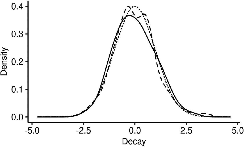
Figure 1.
Remarkable uncertainty in fitted decay parameter values. We illustrate the normalized distribution of decay values estimated with L-BFGS-B across 100 realizations of the same Hawkes process (solid line). The discrepancy between that distribution and the standard Gaussian distribution (dotted line) suggests unique uncertainty in Hawkes process decay estimations. Fitting the decay parameter in Hawkes processes with breaks in stationarity results in other kinds of uncertainty (cf. dashed line).
Problem
While baseline and jump parameters of Hawkes processes are typically derived via convex optimization, the estimation of decay parameters in exponential kernels remains an open issue. Previous work simply assumed the decay parameters to be constants [18, 3, 12], cross-validated decay parameter values [17, 11, 39], or estimated them with a range of different optimization approaches [35, 13, 4, 48, 29, 19, 40]. Such estimation approaches result in point estimates that can be considered as sufficient for simulating and predicting event streams. However, researchers frequently interpret Hawkes process parameters directly [34, 5, 48, 44], e.g., to infer the directions of temporal dependency [28, 46, 23]. Even though such applications rely on estimates of decay parameter values, the current state-of-the-art neglects that, in practice, we derive these values only within a degree of certainty, in particular in a common case of a small number of realizations of a given process. This can lead to qualitatively inaccurate conclusions if researchers do not quantify the uncertainty of decay parameter estimates. Moreover, there are only initial studies [36, 40] on how exponential growth, exogenous shocks to a system, or changes in the underlying process mechanics compromise key stationarity assumptions and aggravate estimation errors.
In Fig. 1, we illustrate this problem in relation to a commonly used nonlinear optimization approach for fitting the decay, L-BFGS-B [10]. We estimate the decay value in two cases: (i) a small number of realizations, and (ii) change of process parameters due to a stationarity break. The solid line in the figure represents the normalized distribution of the fitted decay parameter for case (i). We observe that line deviates remarkably from the standard Gaussian depicted as a dotted line, suggesting the need to account for the uncertainty surrounding Hawkes process decay parameter estimations. Repeating the same fitting procedure for case (ii), we observe, in the dashed line, yet other distributional properties of fitted decay values. This suggests a specific need to separately account for uncertainty in the decay parameter estimation in the presence of breaks in stationarity.
This work
The contribution of this paper is two-fold: First, we focus on the potential uncertainty in the decay parameter of Hawkes processes and explore its sources and consequences. In that regard, we uncover that the non-convex and noisy shape of the Hawkes process log-likelihood as a function of the decay is one cause of the variability in decay parameter estimates. Second, we propose to integrate the estimation of the decay parameter in a Bayesian approach. This allows for (i) quantifying uncertainty in the decay parameter, (ii) diagnosing estimation errors, and (iii) addressing breaks of the crucial stationarity assumption. In our approach, we formulate and evaluate closed-form and intractable hypotheses on the value of the decay parameter. Specifically, we encode hypotheses for the decay as parameters of a prior distribution. Then, we consider estimations of the decay for single Hawkes process realizations as samples from a likelihood. These likelihood samples form the data that we combine with the prior to perform Bayesian inference of posterior decay values.
We show with synthetic data as well as in a broad range of real-word domains that our Bayesian inference procedure for fitting the decay parameter allows for quantifying uncertainty, diagnosing estimation errors, and analyzing breaks in stationarity. In our first application, a study of earthquakes in Japanese regions [34], we uncover low uncertainty in certain geographical relationships. Second, we support Settles and Meeder’s [41] hypothesis that vocabulary learning effort on the Duolingo mobile app correlates to the estimated difficulty of the learned words [33]. Finally, leveraging a dataset of Tweets before and after the Paris terror attacks of November 2015, we measure the relation between a stationarity-breaking exogenous shock and collective effervescence [20].
Overall, our work sheds light on fitting a widely used class of Hawkes processes, i.e., Hawkes processes with exponential kernels. Better understanding these models and explicitly surfacing uncertainty in their fitted values facilitates their use by practitioners and researchers. We expect the impact of our study to be broad,11 as our results influence the application of a key analysis approach for studying time-dependent phenomena across most diverse domains such as seismology, finance, or online communities.
2.Related work
Framed in a broad context, our work complements literature on temporal data analysis methods and applications. Temporal data analysis often models phenomena of interest as time series for tasks such as, prominently, prediction [27], outlier detection [21] or similarity search [49]. In particular, the latter is the goal of the broad research stream on time series representation methods (cf. Lin et al.’s [31] citation graph), which derive compact symbolic representations for segments of a time series. Crucially, such representation and segmentation approaches also facilitate the analysis of a more general class of temporal data, where, in contrast to time series, events are not equally spaced in time. To learn from such data, which we term event streams, previous research proposes, for example, (1) deriving binary codes to infer directions of causality between event streams [9], (2)detecting multiple levels of temporal granularity via self-adapting segmenting of event streams [30], (3) or dynamically defining differently sized temporal windows to cluster users of recommender systems [50]. Complementing that research, we demonstrate how to model irregular temporal signatures with Hawkes processes, thus providing a stepping stone for future work to incorporate, rather than discretize, such information. Applications such as Aghababaei and Makrehchi’s [1] predictions of crime trends from Twitter data, or Rocha and Rodrigues’ [37] forecasts of emergency department admissions could benefit from our approach by capturing rich signals embedded in the event times of Tweets or of hospital admissions. Thus, much like Tai and Hsu [45] with their study on commodity price prediction with deep learning, we also provide guidance for practitioners to apply Hawkes processes. Finally, on the methodological side, we also complement existing research highlighting challenges and approaches to learn from non-stationary data [38].
We now position our work within the more specific context of Hawkes process research. One of the first fields to leverage the seminal work by Hawkes [24] includes seismology [34, 14]. Since then, Hawkes process theory and practice emerged in the realm of finance [5, 4, 46], as well as, more recently, in modeling user activity online [52, 53, 48, 44, 36, 29, 43, 40, 28, 23]. More specifically, the latter body of work extended Hawkes processes to predict diffusion and popularity dynamics of online media [53, 52, 36], model online learning [48, 43], capture the spread of misinformation [44], and understand user behavior in online communities [40, 28], in online markets [23] and in the context of the offline world [29]. As all of those previous references interpreted the parameter values of Hawkes processes (and variations thereof), they may benefit from our study of the decay parameter, especially as we uncover its properties and assess and mitigate estimation issues with Bayesian inference.
Perhaps closest to our work is Bacry et al.’s [4] study of mean field inference of Hawkes process values. In particular, those authors inspected the effect of varying the decay parameter across a range of values: With increasing decay, fitted self- and cross-excitations decrease while baseline intensity increases. We go beyond their study by deepening our understanding of the (noisy) properties of the Hawkes log-likelihood as a function of the decay. Methodologically, our Bayesian approach relates to Hosseini et al.’s [25]. Those authors infer the decay parameter by assuming a Gamma prior and computing the mean of samples from the posterior (as part of a larger inference problem). In our work, we instead focus on the Bayesian approach as a means to quantify estimation uncertainty. Further, as our Bayesian changepoint model captures breaks in stationarity, we simplify previous work [36, 40] which relies on additional assumptions, such as estimating stationarity via the time series of event counts. Our work also complements recent efforts [46] to learn Hawkes processes from small data.
3.Decay estimation in hawkes processes
In this section, we first summarize fundamentals of Hawkes process modelling before describing the problem of decay estimation.
3.1Hawkes processes
We briefly discuss temporal point processes, a set of mathematical models for discrete events randomly arriving over time. Temporal point processes capture the time of an upcoming event given the times of all previous events via the so-called conditional intensity function (or simply intensity)
(1)
where
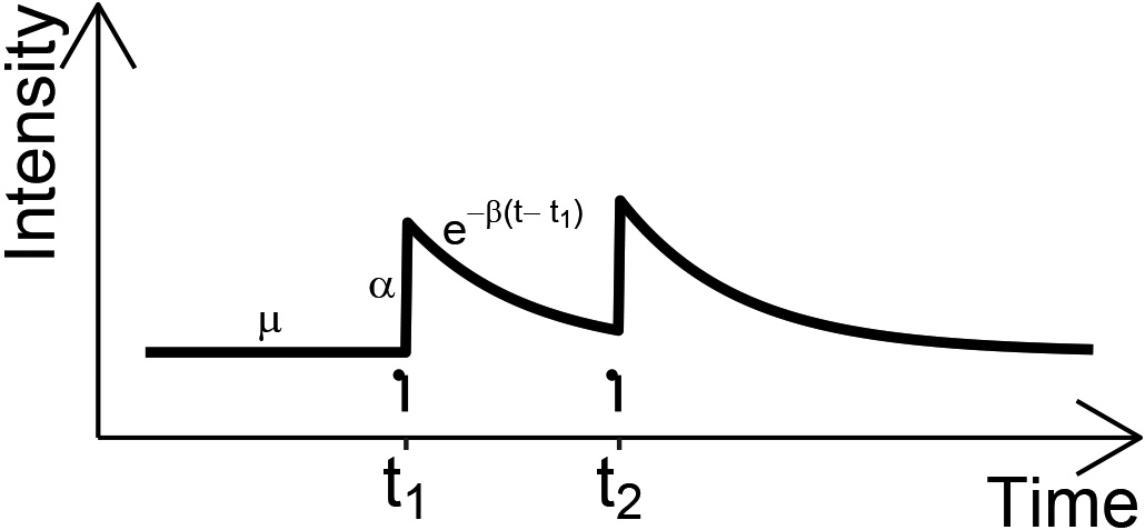
Figure 2.
Illustration of hawkes process intensity
Hawkes processes [24] assume
(2)
where
(3)
which we illustrate in Fig. 2.
Multivariate Hawkes processes with an exponential kernel generalize univariate ones by introducing parameters for self-excitation and for the decay per dimension. Beyond self-excitation, they also capture cross-excitation, the intensity jump an event in one dimension causes in another. Formally, the intensity of dimension
(4)
Notice that we index each dimension’s intensity function with
We now introduce the notions of stationarity and causality in the multi-dimensional Hawkes process context. Stationarity implies translation-invariance in the Hawkes process distribution, and, in particular, it also implies that the intensity does not increase indefinitely over time and therefore stays within bounds. More formally, a Hawkes process with an exponential kernel is stationary if the spectral radius
Recent work [16] established a connection between Granger causality and the excitation matrix: In the particular case of our exponential kernel, dimension
Finally, we define the Hawkes process likelihood function. We work with the log-likelihood function due to its mathematical manipulability and to avoid computational underflows. The equation for the one-dimensional log-likelihood of the Hawkes process with an exponential kernel is as follows [35]:
(5)
with
Ozaki [35] also proposes a (computationally less intensive) recursive formulation for Eq. (5). We refer the interested reader to Daley and Vere-Jones [14] for a general formulation of the log-likelihood of multivariate temporal point processes. Henceforth, as we focus on Hawkes processes with exponential kernels, we refer to them simply as Hawkes processes.
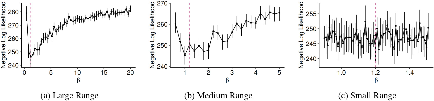
Figure 3.
The negative log-likelihood of hawkes processes as a function of
3.2Decay estimation
To learn from streams of events, practical applications start by fitting Hawkes processes, i.e., optimizing the log-likelihood given in Eq. (5) to a set of event timestamps. Practitioners then inspect fitted parameters to understand inherent temporal dependencies, and perform downstream tasks such as prediction via simulation of the fitted processes [29, 40]. As inferring and interpreting (all) fitted Hawkes process parameters is crucial in many real-world applications [34, 5, 44, 48, 40, 28, 23], we turn our attention to the challenges in fitting Hawkes process parameters, and especially, in estimating the decay parameter in the exponential kernel. Previous research has shown that the baseline
Previous work suggested a wide range of methods to address the decay estimation problem with approaches that provide point estimates. These approaches include setting
We argue that aforementioned problems in estimating decay parameters (cf. Fig. 1) are caused by a noisy, non-convex log-likelihood in
4.Bayesian decay estimation
In this section, we present a novel Bayesian approach for the decay parameter estimation in Hawkes process. We begin with the overall goals and the intuition behind our approach before formally introducing the approach and its operationalization. We also provide a short reflection on a frequentist alternative.
Goals
The aim of our approach is threefold. Firstly, we try to explicitly quantify
Intuition
To that end, we propose a parsimonious Bayesian inference procedure for encoding and validating hypotheses on likely values for
[h] ParamParamInputInputOutputOutputSetupSetup AppendAPPEND FitFIT_DECAY UpdatePosteriorUPDATE_POSTERIOR Stream of
A key difference between our approach and typical applications of Bayesian inference can intuitively be described as follows: The classical Bayesian inference setup typically places a prior distribution for an unknown parameter of interest in a probability distribution which captures the likelihood of given data. Then, applying Bayes’ theorem allows for inferring likely values of the unknown parameter given the data. In our approach, we assume the unknown parameter, i.e., the decay parameter, is also the data, which consists of the aforementioned sequence of decay parameter estimations. This setup enables the freedom to choose between computing posterior (i.e., in parameter space) or posterior predictive (i.e., in data space) distributions to learn about the decay. We find that this flexibility is useful and can improve performance in applications.
Formalization
Given data
(6)
where
(7)
We can also derive credible intervals – roughly Bayesian counterparts of the frequentist confidence interval – for such statistics.
Operationalization
Thus, this setup leaves us with the task of deciding on appropriate distributions for the prior and the likelihood, as well as mapping hypotheses to specific parametrizations of the prior. While we are, in general, free to choose from the broad spectrum of available techniques for Bayesian inference, we propose to assume the likelihood
So far, we focused the presentation of our approach on univariate Hawkes processes. To generalize to the multivariate case, we set
A frequentist alternative
Finally, we reflect on a bootstrap-based alternative formulation of our Bayesian approach. Repeatedly resampling
5.Experiments
We illustrate experimentally how our approach allows for quantifying the uncertainty in the decay and other Hawkes process parameter values, diagnosing mis-estimation and addressing breaks in stationarity. For each of those three goals, we illustrate how our approach achieves the goal (i) with a synthetic dataset and (ii) within a real-world application. We summarize dataset characteristics for each of those goals in Table 1. Overall, we demonstrate that, besides achieving the previously mentioned goals, our approach is broadly applicable across practical scenarios.
Table 1
Dataset characteristics per goal
| Goal | Dataset type | Number of realizations | Mean number of events per realization |
|---|---|---|---|
| Quantify Uncertainty | Synthetic | 100 | 2140 |
| Real-World | 4 | 19 | |
| Diagnose Mis-Estimation | Synthetic | 100 | 100 |
| Real-World | 56 | 10 | |
| Address Stationarity Breaks | Synthetic | 100 | 100 |
| Real-World | 410 | 22 |
5.1Quantifying the uncertainty
We begin by addressing the problem of quantifying the uncertainty of fitted decay values
Synthetic data
We consider a two dimensional Hawkes process with parameters
Figure 4.
Quantifying uncertainty when inferring directions of influence. We first fit
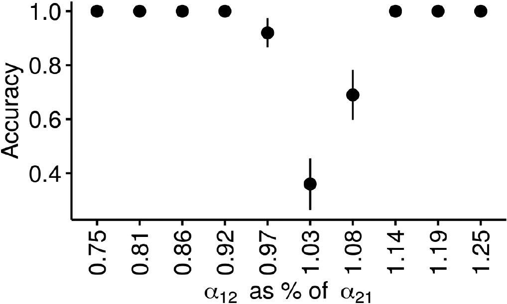
Figure 4 summarizes the outcome of this experiment. As expected, we observe lower accuracies in inferring the direction of influence between dimension 1 and dimension 2 for
Earthquakes and aftershocks
We illustrate the outlined uncertainty quantification procedure with a dataset of earthquakes in the Japanese regions of Hida and Kwanto, as initially studied by Ogata et al. [34]. We consider the data listed in Table 6 of that manuscript, i.e., a dataset of 77 earthquakes from 1924 to 1974. We employ the decay value listed in Table 5 of that manuscript as the prior’s parameter in our closed-form Bayesian approach.66 We assume a two-dimensional Hawkes process with a single
We replicate the seismological relationship that earthquakes in the Japanese Hida region precede those in Kwanto, as we obtain
5.2Mis-estimation & misaligned hypotheses
In this section, we demonstrate that our Bayesian approach facilitates diagnosing (inevitable) estimation errors and misaligned hypotheses as over- or under-estimates, as well as the magnitude of that error. Hence, we address a need, which previous work [34, 4, 48] implies, to encode, validate and diagnose estimations and hypotheses on the decay parameter value. Again, we illustrate how our approach meets that need with synthetic and real-world data.
Synthetic data
We consider a univariate Hawkes process with parameters
We observe that L-BFGS-B and Hyperopt return the decay estimates with lowest RMSE, while Grid Search performs remarkably worse. Aiming to reduce RMSE across all approaches, we inspect the estimates more closely. Looking into
Vocabulary learning intensity
We investigate a scenario proposed as future work by Settles and Meeder’s [41] study of user behavior on the Duolingo language learning app: The authors speculate that vocabulary learning intensity in Duolingo correlates with word difficulty as defined by the CEFR language learning framework [33]. We complement the Duolingo data with a dataset of English-language vocabulary and its corresponding CEFR level,77 and we build two groups of words: those from the easiest CEFR levels, A1 and A2 (A-level group), and those from the hardest ones, C1 and C2 (C-level group). We observe that there are 28 users with 10 vocabulary learning events in the C-level. To control for total learning events per user, we randomly sample a set of 28 users with 10 learning events in the A-level. Increasing the number of events to 11 or 12 leads to qualitatively similar results, but decreased statistical power due to smaller sample size. We repeat this random sampling for a total of 100 times to Bayesian bootstrap 95% credible intervals. We posit that each Duolingo user learning the A-level set of words represents a realization of a univariate Hawkes process, and users learning the C-level words represent realizations of another univariate Hawkes process. Mapping the six CEFR levels (A1, A2, B1, B2, C1 and C2) to a scale from 1 to 6, we naively assume, for illustration purposes, that the C-levels may be more than twice as hard as A-levels. If the data reflects that hypothesis, then we expect that a short learning burst suffices for grasping A-level words, in contrast to the C-level words, which may require perhaps more than two times as much effort over time. We encode this hypothesis in our closed-form Bayesian approach (with L-BFGS-B) as
Figure 5.
In the Duolingo app, users learning C-level words have longer learning bursts than those learning A-level words. We fit two Hawkes processes to users with 10 word learning events on Duolingo: one for users studying “hard” (C-level) words, and the other for users learning “easy” (A-level) words. We posit that the decay value of the C-level process is half as large as the A-level one, and we depict the ratio of the former to the latter. The ratio of fitted values (“Fitted Decay Ratio”) is lower than that of posterior predictive density means (“Bayesian Decay Ratio”), due to a conservative prior parametrization. Lower decay values for the same number of events imply longer event bursts, suggesting that C-level words require extended learning effort.
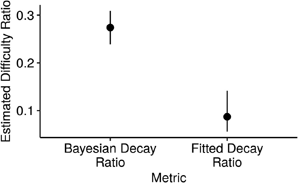
In Fig. 5, we depict the ratio of posterior predictive density means
5.3Addressing breaks in stationarity
We turn our attention to the assumption of stationarity and its effect on fitting the decay parameter of Hawkes processes. Recall that stationarity implies that the intensity of a Hawkes process is translation-invariant. In practical applications such as the study of virality of online content [36] or the growth of online communities [40], exogenous shocks or exponential growth break the stationarity assumption. With synthetic data and a real-world example, we show how our Bayesian approach allows for assessing and capturing breaks in stationarity caused by exogenous shocks.
Synthetic data
We start with the same experimental setup as in Section 5.2, but we introduce two key differences. First, we assume that there was an underlying change in
As a side result, we note that L-BFGS-B and Hyperopt again outperform Grid Search with respect to RMSE. Further, we report mean accuracy values close to 1 for Hyperopt and L-BFGS-B (both 0.98
Strength of collective effervescence
Our third real-world scenario concerns the manifestation of collective effervescence on Twitter in response to the 13. November 2015 terrorist attacks in Paris, as studied by Garcia and Rimé [20]. They proposed future work could analyze how tweet timings reflect collective emotions surrounding the attacks. We address this suggestion by fitting the changepoint Bayesian model with the L-BFGS-B method. Specifically, we begin by extracting the timestamps of tweets by users in a two week period centered on the day of the attacks. We model each user’s behavior per week as a realization of a univariate Hawkes process, and we also control for tweeting activity per user: We extract all 205 users who tweeted between 20 and 25 times in the week before and in the week after.88 Lowering the activity bounds yields more users each with less events to fit, while increasing those bounds has the opposite effect. However, by setting the activity bounds to different ranges of 5 tweets (specifically, 10 to 15, 15 to 20, …, or 45 to 50 tweets), we qualitatively observe the same outcomes. We hypothesize that Twitter users, who partake in the collective emotion as a reaction to the shock, feature a sustained burst of activity. We expect such a burst of activity to translate into a decrease of the decay value after the shock. To numerically capture this hypothesis, we simply set
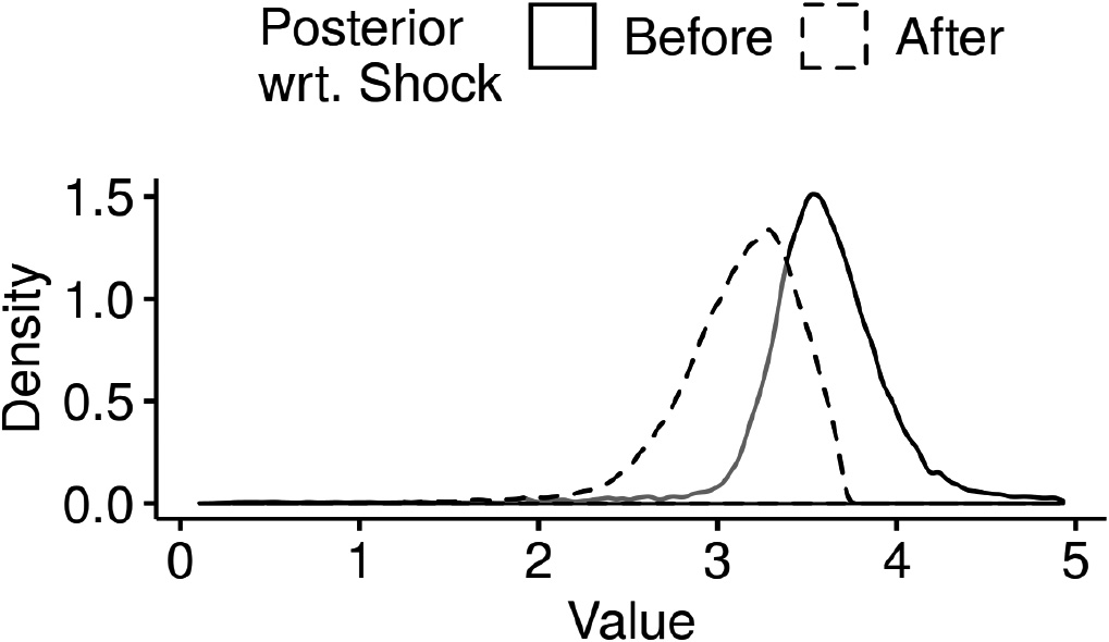
Figure 6 depicts the density of the distribution of the inferred decay posterior before and after the shock. As expected, we confirm the decay value goes down in the week after the attacks, suggesting more sustained bursts of Tweeting activity in response to the attacks. This, in turn, supports the hypothesis that Garcia and Rimé advanced: Reaction timings, in the form of longer bursts of tweets afforded by a 15% lower mean posterior decay after the shock, reflect this collective emotion. We note that this is a conservative estimate of the decrease in the parameter, since activity levels quickly revert back to a baseline within the week after the attacks themselves, as Garcia and Rimé report. Further, this changepoint detection approach also over-estimates the time of the change at realization number 235, i.e., 7.1% later than the first Hawkes process realization after the shock, corresponding to realization number 206.
Figure 6.
Tweet timing reflects collective emotions. We depict the result of fitting an MCMC-based changepoint detection model to users’ Tweet timings in the two weeks surrounding the November 2015 Paris attacks: The estimated posterior density for the Hawkes process intensity decay assigns more probability mass to higher decay regions before the shock in comparison to afterwards. This suggests that collective effervescence manifests on Tweet timings, as lower decay values after the shock reflect more sustained bursts of activity.
6.Discussion
We reflect on practical aspects of our Bayesian approach vs. a frequentist alternative. Bayesian and frequentist inference are two intensively discussed alternative statistical schools for estimating parameters. In recent years, Bayesian approaches received increasing appreciation by the web and machine learning communities (e.g. [7, 51, 42]). Beyond that body of work and theoretical considerations (cf. also Sec. 4), we outline practical differences between our Bayesian approach and a bootstrap-based frequentist alternative. Quantifying the uncertainty of decay estimates with bootstrap amounts to deriving confidence (rather than credible) intervals for the decay from the empirical bootstrap distribution. Diagnosing mis-estimates and misaligned hypotheses with the bootstrapped decay distribution is not an integral part of the frequentist inference procedure, on the contrary to our Bayesian approach, which integrates the hypothesis in the inference procedure. However, explicitly formulating one- or two-sided statistical hypotheses to be tested against the bootstrap distribution is just as viable. In the case of addressing breaks of stationarity, the bootstrap-based approach features remarkably higher complexity than our proposed Bayesian approach. While we infer all three parameters capturing the stationarity break simultaneously, the straightforward bootstrap-based alternative would require alternatively computing the distribution of one parameter while fixing the other two (as the inferred distribution is intractable). Hence, we argue that our Bayesian approach may also be the more natural choice for intractable inference. Nevertheless, we stress that the frequentist alternative we outlined is a viable alternative to our Bayesian approach.
7.Conclusion
In this work, we studied the problem of fitting the decay parameter of Hawkes processes with exponential kernels. The inherent difficulties we found in accurately estimating the decay value, regardless of the fitting method, relate to the noisy, non-convex shape of the Hawkes log-likelihood as a function of the decay. Further, we identified problems in quantifying uncertainty and diagnosing fitted decay values, as well as in addressing breaks of the stationarity assumption. As a solution, we proposed a parsimonious Bayesian approach. We believe our extensive evaluation of that approach across a range of synthetic and real-world examples demonstrates its broad practical use.
Optimization techniques such as constructing convex envelopes or disciplined convex-concave programming may, in the future, help to optimize the Hawkes process likelihood as a function of the decay. We also believe exploring the potential of the vast Bayesian statistics toolbox for learning more from fitted (decay) parameter values is promising future work.
Notes
1 We make our code available at https://github.com/tfts/hawkes_exp_bayes.
2 Note that the set
3 We suggest choosing likelihood distributions with positive support as
4 We recommend using empirical bootstrap statistics to correct for sample bias.
5 We report bootstrap statistics here to refrain from unnecessarily extending our Bayesian approach to the other Hawkes process parameters, which, as previously mentioned, should be estimated with convex optimization routines.
6 We choose that prior for demonstration purposes, as that decay value was estimated with a different Hawkes process from the one we study in this work.
8 Note that this extraction process results in a total of 410 realizations, i.e., 205 realizations before the shock and another 205 afterwards. The mean number of events per realization is 22.
Acknowledgments
We thank David Garcia for giving access to the extended Twitter data. We also thank Roman Kern for valuable feedback on the manuscript. Tiago Santos was a recipient of a DOC Fellowship of the Austrian Academy of Sciences at the Institute of Interactive Systems and Data Science of the Graz University of Technology.
References
[1] | S. Aghababaei and M. Makrehchi, Mining twitter data for crime trend prediction, Intelligent Data Analysis, (2018) . |
[2] | Y. Aït-Sahalia, J. Cacho-Diaz and R. Laeven, Modeling financial contagion using mutually exciting jump processes, Journal of Financial Economics, (2015) . |
[3] | E. Bacry, M. Bompaire, P. Deegan, S. Gaïffas and S. Poulsen, Tick: a python library for statistical learning, with an emphasis on hawkes processes and time-dependent models, The Journal of Machine Learning Research, (2018) . |
[4] | E. Bacry, S. Gaïffas, I. Mastromatteo and J.-F. Muzy, Mean-field inference of hawkes point processes, Journal of Physics A: Mathematical and Theoretical, (2016) . |
[5] | E. Bacry, I. Mastromatteo and J.-F. Muzy, Hawkes processes in finance, Market Microstructure and Liquidity, (2015) . |
[6] | A.-L. Barabasi, The origin of bursts and heavy tails in human dynamics, Nature, (2005) . |
[7] | D. Barber, Bayesian reasoning and machine learning, Cambridge University Press, (2012) . |
[8] | J. Bergstra, R. Bardenet, Y. Bengio and B. Kégl, Algorithms for hyper-parameter optimization, in: NeurIPS, (2011) . |
[9] | K. Budhathoki and J. Vreeken, Causal inference on event sequences, in: SDM, (2018) . |
[10] | R. Byrd, P. Lu, J. Nocedal and C. Zhu, A limited memory algorithm for bound constrained optimization, SIAM Scientific Computing, (1995) . |
[11] | E. Choi, N. Du, R. Chen, L. Song and J. Sun, Constructing disease network and temporal progression model via context-sensitive hawkes process, in: ICDM, (2015) . |
[12] | J. Choudhari, A. Dasgupta, I. Bhattacharya and S. Bedathur, Discovering topical interactions in text-based cascades using hidden markov hawkes processes, in: ICDM, (2018) . |
[13] | J. Da Fonseca and R. Zaatour, Hawkes process: Fast calibration, application to trade clustering, and diffusive limit, Journal of Futures Markets, (2014) . |
[14] | D. Daley and D. Vere-Jones, An Introduction to the Theory of Point Processes: Elementary Theory of Point Processes, Springer, (2003) . |
[15] | B. Efron and T. Hastie, Computer age statistical inference, CUP, (2016) . |
[16] | J. Etesami, N. Kiyavash, K. Zhang and K. Singhal, Learning network of multivariate hawkes processes: A time series approach, in: UAI, (2016) . |
[17] | M. Farajtabar, N. Du, M. Gomez-Rodriguez, I. Valera, H. Zha and L. Song, Shaping social activity by incentivizing users, in: NIPS, (2014) . |
[18] | M. Farajtabar, Y. Wang, M. Gomez-Rodriguez, S. Li, H. Zha and L. Song, Coevolve: A joint point process model for information diffusion and network co-evolution, in: NeurIPS, (2015) . |
[19] | F. Figueiredo, G. Borges, P. de Melo and R. Assunção, Fast estimation of causal interactions using wold processes, in: NeurIPS, (2018) . |
[20] | D. Garcia and B. Rimé, Collective emotions and social resilience in the digital traces after a terrorist attack, Psychological Science, (2019) . |
[21] | M. Gupta, J. Gao, C. Aggarwal and J. Han, Outlier detection for temporal data: A survey, IEEE Transactions on Knowledge and data Engineering, (2013) . |
[22] | T. Hastie, R. Tibshirani and J. Friedman, The elements of statistical learning: Data mining, inference, and prediction, Springer Science & Business Media, (2009) . |
[23] | T. Hatt and S. Feuerriegel, Early detection of user exits from clickstream data: A markov modulated marked point process model, in: WWW, (2020) . |
[24] | A. Hawkes, Spectra of some self-exciting and mutually exciting point processes, Biometrika, (1971) . |
[25] | S. Hosseini, A. Khodadadi, A. Arabzadeh and H. Rabiee, Hnp3: A hierarchical nonparametric point process for modeling content diffusion over social media, in: ICDM, (2016) . |
[26] | J. Hulstijn, The shaky ground beneath the cefr: Quantitative and qualitative dimensions of language proficiency, The Modern Language Journal, (2007) . |
[27] | R. Hyndman and G. Athanasopoulos, Forecasting: Principles and Practice, OTexts, (2018) . |
[28] | R. Junuthula, M. Haghdan, K. Xu and V. Devabhaktuni, The block point process model for continuous-time event-based dynamic networks, in: WWW, (2019) . |
[29] | T. Kurashima, T. Althoff and J. Leskovec, Modeling interdependent and periodic real-world action sequences, in: WWW, (2018) . |
[30] | H. Li and Y. Yu, Detecting a multigranularity event in an unequal interval time series based on self-adaptive segmenting, Intelligent Data Analysis, (2021) . |
[31] | J. Lin, E. Keogh, S. Lonardi and B. Chiu, A symbolic representation of time series, with implications for streaming algorithms, in: SIGMOD Workshop on Research Issues in Data Mining and Knowledge Discovery, (2003) . |
[32] | T. Liniger, Multivariate Hawkes Processes, PhD thesis, ETH, (2009) . |
[33] | C. of Europe, Common European Framework of Reference for Languages: Learning, Teaching, Assessment, Cambridge University Press, (2001) . |
[34] | Y. Ogata, H. Akaike and K. Katsura, The application of linear intensity models to the investigation of causal relations between a point process and another stochastic process, Annals of the Institute of Statistical Mathematics, (1982) . |
[35] | T. Ozaki, Maximum likelihood estimation of hawkes’ self-exciting point processes, Annals of the Institute of Statistical Mathematics, (1979) . |
[36] | M.-A. Rizoiu, L. Xie, S. Sanner, M. Cebrian, H. Yu and P. Van Hentenryck, Expecting to be hip: Hawkes intensity processes for social media popularity, in: WWW, (2017) . |
[37] | C. Rocha and F. Rodrigues, Forecasting emergency department admissions, Journal of Intelligent Information Systems, (2021) . |
[38] | A. Rossi, B. De Souza, C. Soares, A. de Leon Ferreira de Carvalho and C. Ponce, A guidance of data stream characterization for meta-learning, Intelligent Data Analysis, (2017) . |
[39] | F. Salehi, W. Trouleau, M. Grossglauser and P. Thiran, Learning hawkes processes from a handful of events, in: NeurIPS, (2019) . |
[40] | T. Santos, S. Walk, R. Kern, M. Strohmaier and D. Helic, Self- and cross-excitation in stack exchange question & answer communities, in: WWW, (2019) . |
[41] | B. Settles and B. Meeder, A trainable spaced repetition model for language learning, in: ACL, (2016) . |
[42] | P. Singer, D. Helic, A. Hotho and M. Strohmaier, Hyptrails: A bayesian approach for comparing hypotheses about human trails on the web, in: Proceedings of the 24th International Conference on World Wide Web, (2015) , pp. 1003–1013. |
[43] | B. Tabibian, U. Upadhyay, A. De, A. Zarezade, B. Schölkopf and M. Gomez-Rodriguez, Enhancing human learning via spaced repetition optimization, PNAS, (2019) . |
[44] | B. Tabibian, I. Valera, M. Farajtabar, L. Song, B. Schölkopf and M. Gomez-Rodriguez, Distilling information reliability and source trustworthiness from digital traces, in: WWW, (2017) . |
[45] | L. Tai and C. Hsu, On the profitability and errors of predicted prices from deep learning via program trading, Intelligent Data Analysis, (2020) . |
[46] | W. Trouleau, J. Etesami, M. Grossglauser, N. Kiyavash and P. Thiran, Learning hawkes processes under synchronization noise, in: ICML, (2019) . |
[47] | A.C. Türkmen, hawkeslib, github.com/canerturkmen/hawkeslib, (2019) . |
[48] | U. Upadhyay, I. Valera and M. Gomez-Rodriguez, Uncovering the dynamics of crowdlearning and the value of knowledge, in: WSDM, (2017) . |
[49] | X. Wang, A. Mueen, H. Ding, G. Trajcevski, P. Scheuermann and E. Keogh, Experimental comparison of representation methods and distance measures for time series data, Data Mining and Knowledge Discovery, (2013) . |
[50] | C. Xiao, K. Xia, X. Liu, Y. Zhang, W. Huo and N. Aslam, Improving session-based temporal recommendation by using dynamic clustering, Intelligent Data Analysis, (2017) . |
[51] | X. Yang, Y. Guo and Y. Liu, Bayesian-inference-based recommendation in online social networks, IEEE Transactions on Parallel and Distributed Systems 24: (4) ((2012) ), 642–651. |
[52] | K. Zhou, H. Zha and L. Song, Learning social infectivity in sparse low-rank networks using multi-dimensional hawkes processes, in: AISTATS, (2013) . |
[53] | K. Zhou, H. Zha and L. Song, Learning Triggering Kernels for Multi-Dimensional Hawkes Processes, in: ICML, (2013) . |


