
Unsupervised feature extraction from multivariate time series for outlier detection
Abstract
Although various feature extraction algorithms have been developed for time series data, it is still challenging to obtain a flat vector representation with incorporating both of time-wise and variable-wise association between multiple time series. Here we develop an algorithm, called Unsupervised Feature Extraction using Kernel and Stacking (UFEKS), that constructs feature vector representation for multiple time series in an unsupervised manner. UFEKS constructs a kernel matrix for the set of subsequences from each time series and horizontally concatenates all matrices. Then we can treat each row as a feature vector representation of its corresponding subsequence of times series. We examine the effectiveness of the extracted features under the unsupervised outlier detection scenario using synthetic and real-world datasets, and show its superiority compared to well-established baselines.
1.Introduction
Internet of things (IoT) devices, composed of many sensors such as temperature, humidity, and pressure, are installed in various types of systems, and multivariate time series data are being collected in a wide range of fields. For example, in the task of facility maintenance for a building, it may be possible to know the best timing of their replacement by monitoring and analyzing collected data. Although this process, called condition based maintenance (CBM) [12], is well known technology in industrial fields, this task is still challenging as we need to use many multivariate time series to find relationship between sensors. In the case of sensing at multiple locations in a building, sensors located in the same local area are expected to record similar values. If one sensor takes different values from others, the sensor might be broken and need to be replaced to the new one. However, it is hard to find the sensor taking different values because we need to find different combinatorial relationships between sensors.
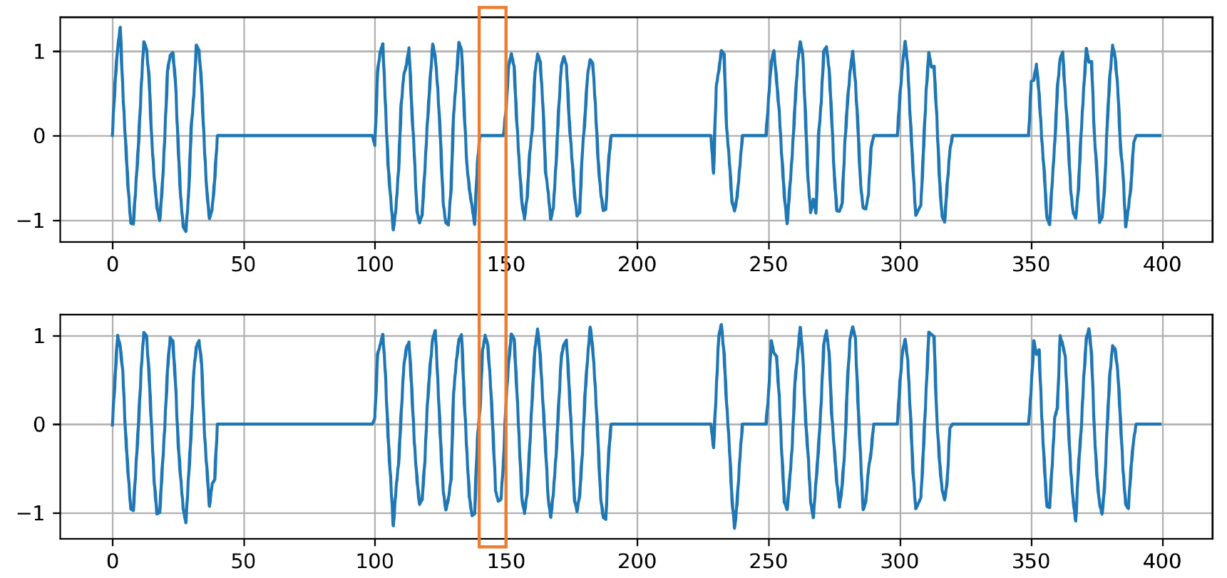
In this paper, we consider association between multiple time series. An example of association is shown in Fig. 1. There are two time series from the corresponding variables composed of lines and sine waves with noise. In an orange frame, the time series is composed of line and sine wave (up and bottom), while the other subsequences out of the orange frame are composed of the combination of only lines or sine waves. Hence only the subsequence in the orange frame has a different combination. This is an example of a combinatorial outlier, and finding such outliers is fundamentally difficult as they cannot be found if we look at each time series separately. In the case of CBM, if building managers find sudden changes of values like the orange frame, they are probably considered as signals of equipment failures and managers can start to inspect their equipment in more detail. Finding a different combination from multivariate time series data is one of the most important tasks in a number of sensor monitoring tasks including CBM.
Figure 1.
An example of association for multivariate time series data.
In this paper, we focus on the task of extracting feature vector representation from multivariate time series data that can incorporate combinatorial association between two or more time series. This approach is unsupervised, hence it enables us to apply general conventional machine learning algorithms to multivariate time series.
To extract feature vectors from multivariate time series, we propose a new algorithm, called UFEKS (Unsupervised Feature Extraction using Kernel and Stacking), and apply it for outlier detection. The proposed method UFEKS uses a kernel method to extract features from multivariate time series. It first divides a given time series into a set of its subsequences, and makes a kernel matrix from each univariate time series. Then it horizontally concatenates all of the kernel matrices. Our idea is to treat each row in the concatenated matrix as a feature vector, which means that each row corresponds to a point in the multidimensional Euclidean space. Our approach allows us to use standard outlier detection algorithms to detect outliers from multivariate time series with considering combinatorial association between two time series. We examine the proposed method using unsupervised outlier detection as it is commonly used in practical situations such as CBM. It should be noted that our proposed method does not use any labeled data for detecting outliers from multivariate time series. Moreover, the UFEKS can be employed for not only outlier detection but other data mining tasks.
To summarize, the main contributions of our work are:
• Our proposed method UFEKS can extract features from multivariate time series with incorporating combinatorial association between time series. The obtained features can be applied to a variety of applications such as outlier detection or other data mining tasks.
• In outlier detection, the proposed method can detect outliers that cannot be found if we look at each of multivariate time series separately.
The remainder of this paper is organized as follows: In Section 2, we discuss related work of our research in terms of feature extraction and outlier detection for time series. In Section 3, we present our algorithm UFEKS and explain combination with outlier detection techniques as one of the applications. In Section 4, we examine performance of UFEKS on synthetic and real-world datasets. Finally, we conclude this paper by including some remarks in Section 5.
2.Related work
To date, several feature extraction algorithms from time series for outlier detection have been developed. Discrete Fourier Transform (DFT), Discrete Wavelet Transform (DWT), and Discrete Cosine Transformation (DCT) are well known algorithms to extract features from time series used in signal processing fields and data mining fields [3, 16, 23]. Other algorithms such as Piece-wise Aggregate Approximation [14, 33, 10], Symbolic Approximation [13], and fundamental statistics like mean and variance are widely used in data mining fields. However, the above algorithms mainly used for signal processing cannot be directory applied to multivariate time series. Kernel methods are also used to extract features from time series [9, 35]. For example, a kernel matrix using the Radial Basis Function (RBF) kernel [9] or the linear kernel [35] from a time series has been used for outlier detection. However, since these approaches use only the integrated signal across multiple time series, they cannot treat combinatorial association of time series. In contrast, our proposal treats each time series separately when we apply kernels, hence we can treat such combinatorial effects.
Outlier detection for time series have been actively studied and a number of methods have been proposed [1, 28, 9, 17, 30, 22, 25]. In particular for outlier detection from a univariate time series, autoregressive moving average (ARMA) and an autoregressive integrated moving average (ARIMA) have been commonly used [28]. They can find outliers from differences between predicted values by ARMA or ARIMA and actual values. However, they are considered to be sensitive to noise, resulting in increasing false positives when the noise level is severe [28, 35]. Dynamic time warping (DTW) is another representative method, which measures similarity between two time series by aligning them [26, 6, 21]. DTW is widely used in a variety of applications because it is robust to different frequencies or lengths. DTW can be used for univariate time series, however, it may not be directly used for multivariate time series.
In terms of outlier detection from multivariate time series, several algorithms have been proposed [9, 17, 30]. Takeishi and Yairi [30] have proposed an algorithm using sparse representation. This method is designed in a supervised manner and requires labeled data. Moreover, they do not focus on combinatorial association between time series and may not detect combinatorial outliers.
Nowadays, a number of outlier detection methods for time series have been proposed based on neural networks [20, 34, 36, 37, 35]. One of the outlier detection methods for multivariate time series is the Multi-Scale Convolutional Recurrent Encoder-Decoder (MSCRED), which is an algorithm using attention-based convolutional long-short time memory [35]. It extracts features and detects outliers from multivariate time series by constructing a kernel matrix. Many algorithms based on neural networks are usually useful and widely used in real world. However, most of neural network based models have many parameters to be tuned, which is fundamentally difficult in the unsupervised setting. Furthermore, they are often designed as supervised, hence ground-truth labels are required to train their models to perform outlier detection.
Numerous algorithms have been proposed so far for outlier detection for non-time series data [1, 2, 27, 8, 11, 32, 36, 37]. Representative algorithms include local outlier factor (LOF),
3.The UFEKS algorithm and outlier detection
We formulate our method UFEKS in Section 3.1, which extracts feature vectors from multivariate time series, and introduce its application to outlier detection in Section 3.2.
3.1Extraction of features from multivariate time series
Many algorithms to extract features from time series have focused on its subsequences [35, 9, 30, 17]. In this paper, we follow the idea of using subsequences and extract features based on the similarity between subsequences. We use a kernel method to measure the similarity between subsequences as it is widely used in data analysis for time series and its effectiveness is well known.
Assume that there are
(1)
where each row
First, we consider extraction of feature vectors from a univariate time series
(2)
where
(3)
where we denote each row vector as
Now we extend our feature vector representation for univariate time series to multivariate time series. First we generate kernel matrices
(4)
and its row vector
(5)
This matrix
The pseudo code of our method UFEKS is shown in Algorithm 3.1.
[h] : The UFEKS algorithm[1]
3.2Outlier detection from multivariate time series
We propose to apply our method UFEKS to the problem of outlier detection from multivariate time series. When we use our method for a multivariate time series
To detect outliers from multivariate time series
(6)
where
4.Experiments
We empirically evaluate our algorithm on synthetic and real-world datasets.
4.1Comparison partners
We compare our algorithm with two feature representation algorithms, the PageRank kernel (PRK), and Subsequence (SS), under four different unsupervised outlier detection algorithms,
(7)
where
(8)
When we denote each element of
(9)
By considering each row in Eq. (9) to be a multidimensional data point, outliers can be detected by conventional algorithms like
4.2Datasets
We prepared nine types of synthetic multivariate time series datasets and six types of real-world multivariate time series datasets shown in Fig. 2 and Table 1. Each synthetic dataset includes two or more time series and outlierness behavior occurs in only one of time series, which are shown as an orange solid area in Figures from 2a to j. Those outliers have simulated spike noises in the real-world. All the nine synthetic datasets are composed of sine waves or straight lines, and Gaussian noise were added to every data point, where noise were generated by Gaussian distribution with zero mean and 0.1 standard deviation
Figure 2.
Examples of synthetic and real-world datasets.
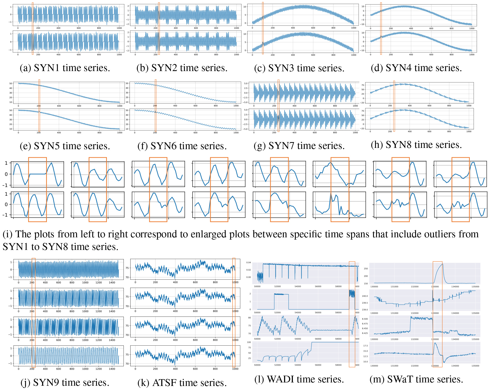
Table 1
Summary of datasets. Datasets between SYN1 and SYN9 are synthetic, and ATSF8, ATSF16, ATSF32, ATSF64, WADI, and SWaT are real-world datasets
| Name of datasets | Number of variables | Range of outliers | Length of time series |
|---|---|---|---|
| SYN1 | 2 | 140–150 | 1,000 |
| SYN2 | 2 | 231–240 | 1,000 |
| SYN3 | 2 | 101–110 | 1,000 |
| SYN4 | 2 | 101–110 | 1,000 |
| SYN5 | 2 | 201–210 | 1,000 |
| SYN6 | 2 | 201–210 | 1,000 |
| SYN7 | 2 | 241–250 | 1,000 |
| SYN8 | 2 | 241–250 | 1,000 |
| SYN9 | 4 | 201–250 | 1,500 |
| ATSF8 | 8 | 951–1,000 | 1,000 |
| ATSF16 | 16 | 951–1,000 | 1,000 |
| ATSF32 | 32 | 951–1,000 | 1,000 |
| ATSF64 | 64 | 951–1,000 | 1,000 |
| WADI | 93 | 9,054–9,644 | 10,000 |
| SWaT | 39 | 2,918–3,380 | 5,000 |
Eight figures from Fig. 2a–h illustrate synthetic multivariate time series datasets, each of which is composed of two time series. Each time series has 1,000 time stamps, and outliers with the length of ten or eleven time stamps are injected. SYN1 time series in Fig. 2a is composed of sine waves and straight line. SYN2 time series in Fig. 2b is composed of two sine waves with different amplitude. Datasets from SYN3 to SYN6 illustrated in Fig. 2c–f are composed of sine waves, and their averages in subsequence are swaying over time. Moreover, a phase shift occurs between their time series in SYN6. SYN7 time series in Fig. 2g is composed of sine waves with different amplitude. SYN8 time series is almost the same as SYN7 except for changes of their averages over time. Enlarged plots between specific time spans that include outliers from SYN1 to SYN8 are shown in Fig. 2i. The SYN9 dataset in Fig. 2j has a set of four time series and each time series has 1,500 time stamps. Their wavelengths of the top and the bottom time series are fifteen and thirty, respectively. The second time series is combined with two wavelengths of ten and twenty. Similarly, the third time series is combined with two wavelengths of ten and twenty-five. Consequently, all of four time series are composed of different wavelengths.
Real-world datasets called ambient temperature system failure (ATSF) are shown in Fig. 2k. Since it is hard to find ground truth combinatorial outliers in multivariate time series from real-world datasets, we collected univariate time series and artificially simulated combinatorial outliers on it. The dataset [4]11 comes from the Numenta Anomaly Benchmark (NAB) v1.1, which is publicly available. We used one of the real-world univariate time series called ATSF, which was ambient temperature in an office setting measured every hour. Although several types of datasets including outliers are available, most of such outliers can be easily detected by checking each time series separately, hence they are not appropriate for our evaluation. Time series we extracted have successive 1,000 time stamps out of 7,267 where it corresponds between November 1, 2013 and December 13, 2013, and we created 8, 16, 32, and 64 variants with adding noise generated by Gaussian distribution with
Furthermore, we employed another types of multivariate time series called Water Distribution (WADI)22 illustrated in Fig. 2l and Secure Water Treatment (SWaT)33 illustrated in Fig. 2m from Singapore University of Technology and Design. Those real-world multivariate time series datasets are also publicly available and outliers have been already included in them. We extracted successive 10,000 out of 172,801 time stamps between 50,001 and 60,000 from WADI datasets, and successive 5,000 out of 449,919 time stamps between 130,000 and 135,000 from SWaT datasets. Their subsets include some outliers that can be obviously and visually identified as outliers. Note that, in comparison with ATSF, we do not artificially inject outliers in both WADI and SWaT datasets.
4.3Environment
We used CentOS release 6.10 with 4x 22-Core model 2.20 GHz Intel Xeon CPU E7-8880 v4 processors and 3.18 TB memory. All methods are implemented in Python 3.7.6 and all experiments are also performed in the same platform.
Table 2
Parameters for algorithms
| Name | Value |
|---|---|
| 5 | |
| 1 | |
| Length of subsequence (SS) | 2 |
4.4Experimental results
We performed three feature representation algorithms: UFEKT, PageRank kernel (PRK), and subsequence (SS), combined with four outlier detection algorithms:
Table 3
Area under precision-recall curve (AUPRC) for synthetic datasets
| OD | LOF | |||||
|---|---|---|---|---|---|---|
| FR | UFEKS | PRK | SS | UFEKS | PRK | SS |
| SYN1 | 0.886 | 0.815 | 0.486 | 0.857 | 0.736 | 0.258 |
| SYN2 | 0.913 | 0.734 | 0.575 | 0.803 | 0.062 | 0.380 |
| SYN3 | 0.980 | 0.625 | 0.016 | 0.953 | 0.118 | 0.011 |
| SYN4 | 0.956 | 0.573 | 0.010 | 0.901 | 0.114 | 0.011 |
| SYN5 | 0.990 | 0.046 | 0.007 | 0.957 | 0.006 | 0.011 |
| SYN6 | 0.237 | 0.063 | 0.182 | 0.023 | 0.007 | 0.139 |
| SYN7 | 0.853 | 0.779 | 0.010 | 0.867 | 0.047 | 0.060 |
| SYN8 | 0.739 | 0.012 | 0.006 | 0.006 | 0.007 | 0.007 |
| SYN9 | 0.375 | 0.368 | 0.033 | 0.140 | 0.069 | 0.035 |
| Average | 0.770 | 0.446 | 0.147 | 0.612 | 0.129 | 0.101 |
| OD | OCSVM | IForest | ||||
| FR | UFEKS | PRK | SS | UFEKS | PRK | SS |
| SYN1 | 0.668 | 0.006 | 0.007 | 0.670 | 0.017 | 0.013 |
| SYN2 | 0.600 | 0.006 | 0.018 | 0.303 | 0.006 | 0.019 |
| SYN3 | 0.418 | 0.006 | 0.008 | 0.017 | 0.006 | 0.011 |
| SYN4 | 0.508 | 0.006 | 0.007 | 0.014 | 0.006 | 0.007 |
| SYN5 | 0.545 | 0.006 | 0.010 | 0.022 | 0.006 | 0.008 |
| SYN6 | 0.008 | 0.007 | 0.008 | 0.007 | 0.007 | 0.014 |
| SYN7 | 0.894 | 0.006 | 0.006 | 0.374 | 0.007 | 0.006 |
| SYN8 | 0.331 | 0.012 | 0.014 | 0.162 | 0.051 | 0.006 |
| SYN9 | 0.117 | 0.020 | 0.032 | 0.070 | 0.030 | 0.032 |
| Average | 0.454 | 0.008 | 0.012 | 0.182 | 0.015 | 0.013 |
Table 4
Area under precision-recall curve (AUPRC) for real-world datasets
| OD | LOF | |||||
|---|---|---|---|---|---|---|
| FR | UFEKS | PRK | SS | UFEKS | PRK | SS |
| ATSF8 | 0.914 | 0.199 | 0.040 | 0.960 | 0.187 | 0.067 |
| ATSF16 | 0.868 | 0.260 | 0.039 | 0.630 | 0.066 | 0.064 |
| ATSF32 | 0.614 | 0.186 | 0.039 | 0.176 | 0.032 | 0.063 |
| ATSF64 | 0.306 | 0.089 | 0.038 | 0.080 | 0.028 | 0.063 |
| WADI | 0.092 | 0.047 | 0.128 | 0.057 | 0.064 | 0.055 |
| SWaT | 0.143 | 0.085 | 0.118 | 0.088 | 0.070 | 0.100 |
| Average | 0.489 | 0.144 | 0.067 | 0.332 | 0.074 | 0.069 |
| OD | OCSVM | IForest | ||||
| FR | UFEKS | PRK | SS | UFEKS | PRK | SS |
| ATSF8 | 0.899 | 0.026 | 0.034 | 0.461 | 0.029 | 0.035 |
| ATSF16 | 0.821 | 0.026 | 0.034 | 0.247 | 0.030 | 0.034 |
| ATSF32 | 0.329 | 0.027 | 0.034 | 0.132 | 0.030 | 0.034 |
| ATSF64 | 0.189 | 0.032 | 0.034 | 0.113 | 0.034 | 0.034 |
| WADI | 0.249 | 0.032 | 0.751 | 0.172 | 0.033 | 0.628 |
| SWaT | 0.783 | 0.118 | 0.881 | 0.643 | 0.054 | 0.365 |
| Average | 0.545 | 0.044 | 0.295 | 0.295 | 0.035 | 0.188 |
Figure 3.
AUPRC of SYN1, SYN2, SYN3, ans SYN4 time series.
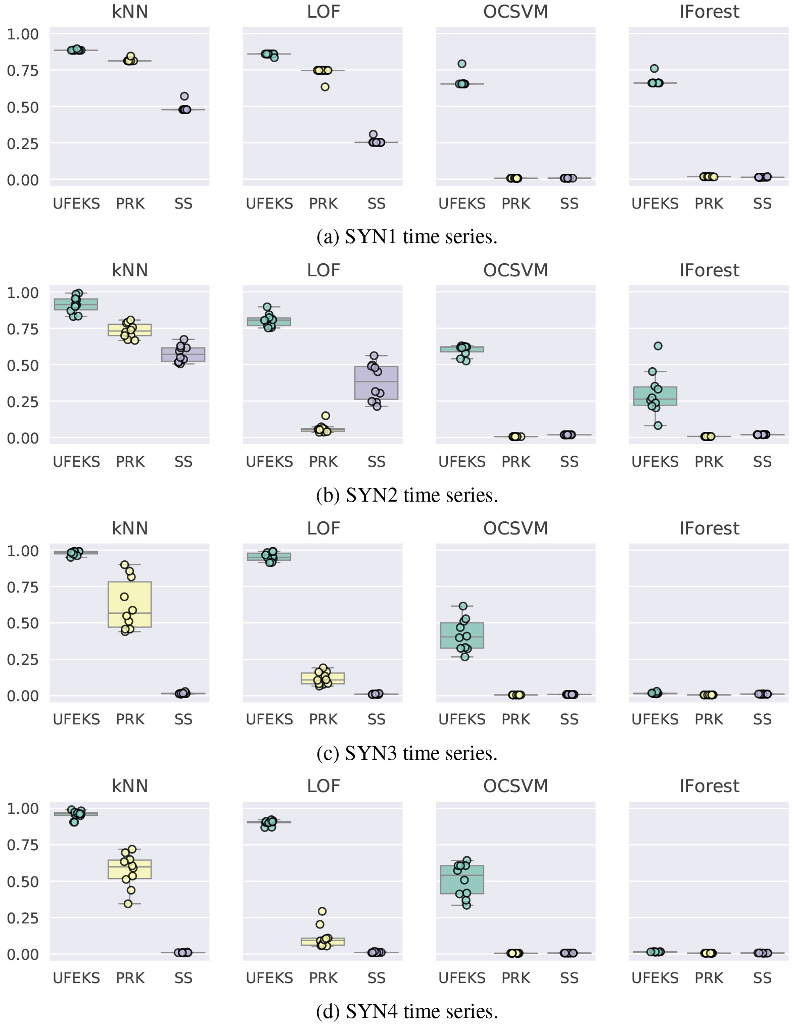
Figure 4.
AUPRC of SYN5, SYN6, SYN7, and SYN8 time series.
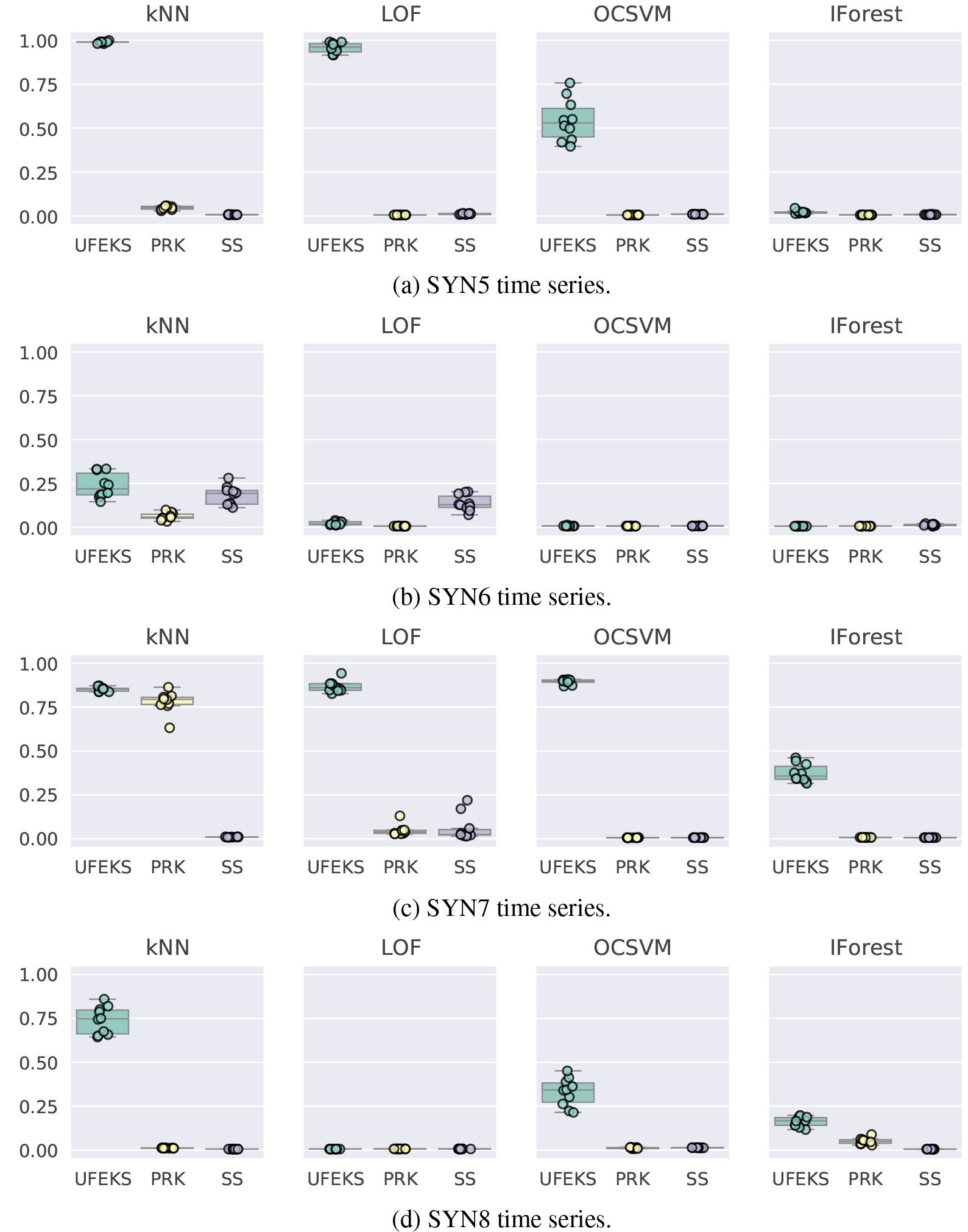
Figure 5.
AUPRC of SYN9, ATSF8, ATSF16, and ATSF32 time series.
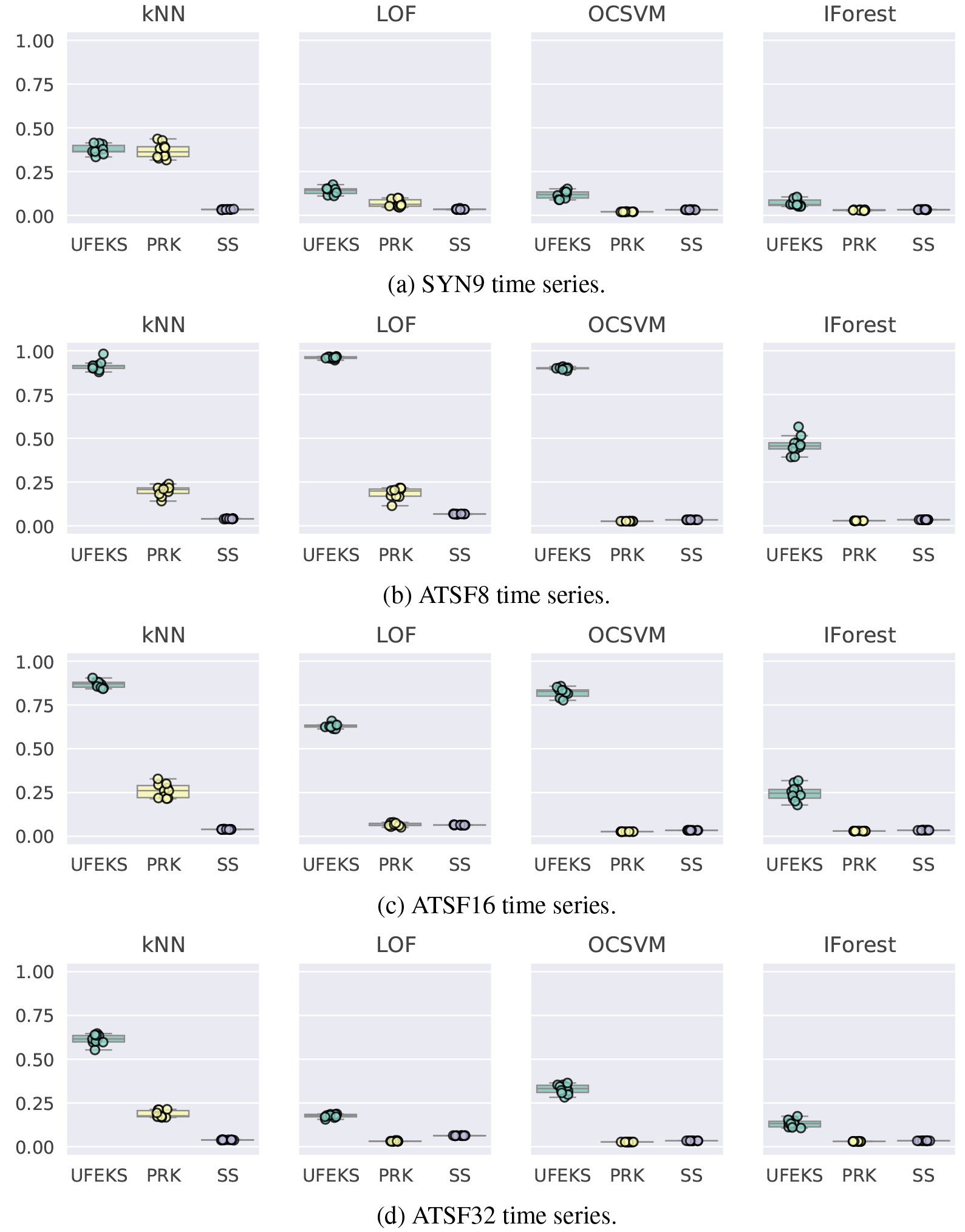
Figure 6.
AUPRC of ATSF64, WADI and SWaT time series.
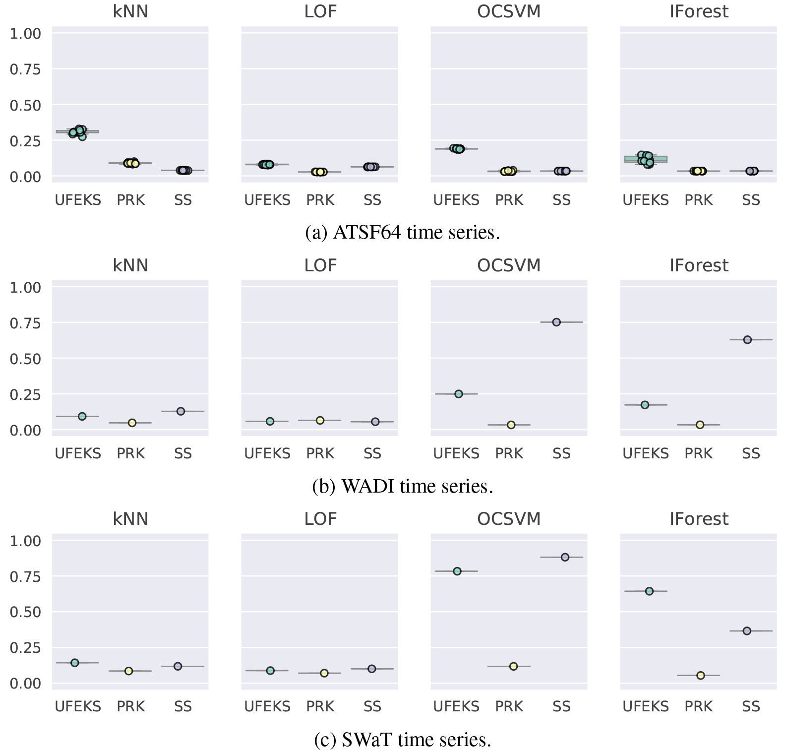
Figure 7.
A result of PCA that is applied to the feature representation obtained by Subsequence (SS) for the SYN7 time series dataset.
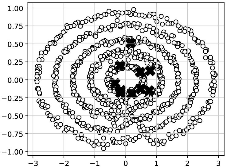
Figure 8.
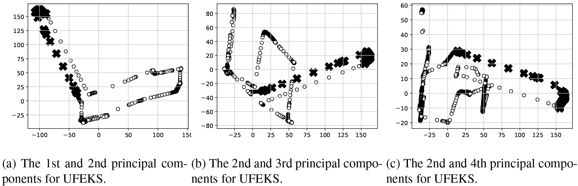
Results of PCA for feature representations obtained by UFEKS (upper row) and PageRank kernel (PRK; lower row) for the SYN7 time series dataset.
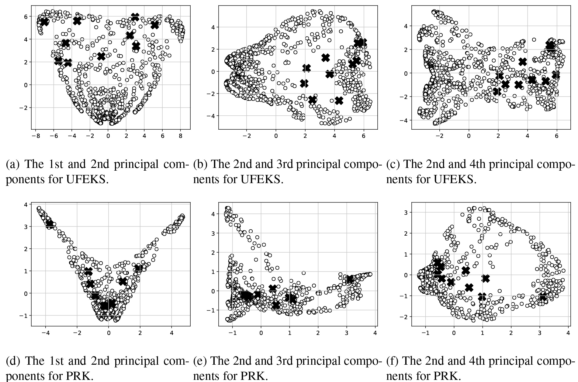
Figure 9.
Results of PCA for the feature representation obtained by UFEKS from SWaT time series.
Results are summarized in Figs 3 and 4, and Tables 3 and 4. OD, FR, PRK, and SS in the figures stand for Outlier Detection, Feature Representation, PageRank Kernel, and SubSequences, respectively. The datasets except for WADI and SWaT are prepared ten patterns for each as we inject Gaussian noises and Mean
4.4.1Synthetic datasets
Figures from Figs 3a to 5a show results of synthetic datasets. There are four plots in each figure and each title in their plots shows the name of the corresponding outlier detection algorithm. Our algorithm, UFEKS, is superior to the other feature representation algorithms PageRank Kernel (PRK) and SubSequence (SS) in all synthetic datasets. In comparison with PRK and SS, our kernel matrix used in the algorithm does not sum up elements in a row of the kernel matrix that represents association between subsequences, while PRK and SS sum up them. Therefore, it is considered that UFEKS has high capability of representing features. Moreover, by using Gaussian kernel, it is expected that UFEKS can reduce noise and extract features easier than SS. Furthermore, it is also interesting that
To analyze difference between feature representation methods deeper, we apply Principal Component Analysis (PCA) for the obtained feature representations from SYN7 datasets as a representative example. The result for Subsequence is plotted in Fig. 7 and those for UFEKS and PageRank kernel are in Fig. 8. The x- and y-axes in Fig. 7 indicate the first and the second principle components, respectively. In Fig. 8, we plot the first and second principle components in the left-hand side plots, the second and third ones for the middle plots, and the second and forth ones for the right-hand side plots. The circles and crosses in all plots denote normal and outlier points, respectively. As the Fig. 7 shows, it seems to be difficult to detect outliers by a conventional algorithm like
4.4.2ATSF datasets
Figures from Figs 5b to 6a show results of ATSF datasets. A detail of the results is shown in Table. 4. The results tend to be similar to synthetic datasets, that is, combinations of
4.4.3WADI and SWaT datasets
Figure 6b and c show results for WADI and SWaT datasets. These results are different from those for the other datasets because OCSVM and IForest have better results than
5.Conclusion
In this paper, we have proposed a new algorithm, called Unsupervised Feature Extraction using Kernel Method and Stacking (UFEKS), to extract features from multivariate time series without any labels. The UFEKS (1) divides a given time series into a set of its subsequences, (2) makes a kernel matrix from each subsequences using the RBF kernel, (3) horizontally concatenates kernel matrices into a single kernel matrix, and (4) extracts row vectors in the concatenated matrix as feature vectors. To evaluate our algorithm, we have applied it to the outlier detection task with four outlier detection methods for non-time series data, such as
Since our method offers a powerful feature extraction scheme that can be applied to any multivariate time series data, it is our interesting future work to apply UFEKS to not only outlier detection but other data mining tasks such as clustering for multivariate time series data.
Notes
Acknowledgments
This work was supported by JST, PRESTO Grant Number JPMJPR1855, Japan and JSPS KAKENHI Grant Number JP21H03503 (MS).
References
[1] | C.C. Aggarwal, Outlier Analysis, Springer, (2017) . |
[2] | C.C. Aggarwal and S. Sathe, Outlier Ensembles, Springer, (2017) . |
[3] | R. Agrawal, C. Faloutsos and A. Swami, Efficient similarity search in sequence databases, in: Lecture Notes in Computer Science, Vol. 730, pages 69–84. (1993) . |
[4] | S. Ahmad, A. Lavin, S. Purdy and Z. Agha, Unsupervised real-time anomaly detection for streaming data, Neurocomputing 262: (nov (2017) ), 134–147. |
[5] | S.D. Bay and M. Schwabacher, Mining Distance-Based Outliers in Near Linear Time with Randomization and a Simple Pruning Rule, in: Proceedings of the 9th ACM SIGKDD International Conference on Knowledge Discovery and Data Mining, pages 29–38, (2003) . |
[6] | D. Berndt and J. Clifford, Using dynamic time warping to find patterns in time series, Workshop on Knowledge Knowledge Discovery in Databases 398: ((1994) ), 359–370. |
[7] | K. Bhaduri, B.L. Matthews and C.R. Giannella, Algorithms for speeding up distance-based outlier detection, in: Proceedings of the ACM SIGKDD International Conference on Knowledge Discovery and Data Mining, number August 2011, pages 859–867, (2011) . |
[8] | V. Chandola, A. Banerjee and V. Kumar, Anomaly detection, ACM Computing Surveys 41: (3) (jul (2009) ), 1–58. |
[9] | H. Cheng, P.-N. Tan, C. Potter and S. Klooster, Detection and Characterization of Anomalies in Multivariate Time Series, in: Proceedings of the 2009 SIAM International Conference on Data Mining, Vol. 1, pages 413–424, apr (2009) . |
[10] | C. Guo, H. Li and D. Pan, An improved piecewise aggregate approximation based on statistical features for time series mining, in: Y. Bi and M.-A. Williams, editors, Knowledge Science, Engineering and Management, pages 234–244, Berlin, Heidelberg, (2010) . Springer Berlin Heidelberg. |
[11] | M. Gupta, J. Gao, C.C. Aggarwal and J. Han, Outlier detection for temporal data: A survey, IEEE Transactions on Knowledge and Data Engineering 26: (9) (sep (2014) ). |
[12] | A.K. Jardine, D. Lin and D. Banjevic, A review on machinery diagnostics and prognostics implementing condition-based maintenance, Mechanical Systems and Signal Processing 20: (7) ((2006) ), 1483–1510. |
[13] | E. Keogh, S. Lonardi and C.A. Ratanamahatana, Towards parameter-free data mining, in: Proceedings of the 2004 ACM SIGKDD International Conference on Knowledge Discovery and Data Mining – KDD ’04, ACM Press, (2004) . |
[14] | E.J. Keogh and M.J. Pazzani, A Simple Dimensionality Reduction Technique for Fast Similarity Search in Large Time Series Databases, in: 4th Pacific-Asia Conference, PAKDD 2000, pages 122–133, (2000) . |
[15] | E.M. Knorr, R.T. Ng and V. Tucakov, Distance-based outliers: Algorithms and applications, The VLDB Journal 8: (3–4) ((2000) ), 237–253. |
[16] | F. Korn, H.V. Jagadish and C. Faloutsos, Efficiently supporting ad hoc queries in large datasets of time sequences, ACM SIGMOD Record 26: (2) (jun (1997) ), 289–300. |
[17] | J. Lee, H.S. Choi, Y. Jeon, Y. Kwon, D. Lee and S. Yoon, Detecting System Anomalies in Multivariate Time Series with Information Transfer and Random Walk, in: Proceedings of 5th IEEE/ACM International Conference on Big Data Computing, Applications and Technologies, pages 71–80, (2018) . |
[18] | F.T. Liu, K.M. Ting and Z.-H. Zhou, Isolation Forest, in: Proceedings of 2008 IEEE International Conference on Data Mining, pages 413–422. IEEE, dec (2008) . |
[19] | J. Ma and S. Perkins, Time-series Novelty Detection Using One-class Support Vector Machines, in: Proceedings of the International Joint Conference on Neural Networks, Vol. 3, pages 1741–1745, (2003) . |
[20] | P. Malhotra, A. Ramakrishnan, G. Anand, L. Vig, P. Agarwal and G. Shroff, LSTM-based Encoder-Decoder for Multi-sensor Anomaly Detection, in: ICML 2016 Anomaly Detection Workshop, (2016) . |
[21] | J. Mei, M. Liu, Y.-F. Wang and H. Gao, Learning a mahalanobis distance-based dynamic time warping measure for multivariate time series classification, IEEE Transactions on Cybernetics 46: (6) (jun (2016) ), 1363–1374. |
[22] | Mingyan Teng, Anomaly detection on time series, in: 2010 IEEE International Conference on Progress in Informatics and Computing, pages 603–608, dec (2010) . |
[23] | F. Mörchen, Time series feature extraction for data mining using DWT and DFT, Technical Report, No. 33, Department of Mathematics and Computer Science, University of Marburg, Germany, pages 1–31, (2003) . |
[24] | A. Munoz and J. Muruzabal, Self-Organizing Maps for Outlier Detection, (1995) . |
[25] | H. Qiu, Y. Liu, N.A. Subrahmanya and W. Li, Granger Causality for Time-Series Anomaly Detection, in: Proceedings of 12th International Conference on Data Mining, pages 1074–1079, (2012) . |
[26] | T. Rakthanmanon, B. Campana, A. Mueen, G. Batista, B. Westover, Q. Zhu, J. Zakaria and E. Keogh, Searching and mining trillions of time series subsequences under dynamic time warping, in: Proceedings of the ACM SIGKDD International Conference on Knowledge Discovery and Data Mining, pages 262–270, (2012) . |
[27] | N.N.R. Ranga Suri, N. Murty and G. Athithan, Outlier Detection: Techniques and Applications, Vol. 155 of Intelligent Systems Reference Library, Springer, (2019) . |
[28] | L. Seymour, P.J. Brockwell and R.A. Davis, Introduction to Time Series and Forecasting, Springer, (2016) . |
[29] | M. Sugiyama and K.M. Borgwardt, Rapid distance-based outlier detection via sampling, in: Advances in Neural Information Processing Systems, pages 1–9, (2013) . |
[30] | N. Takeishi and T. Yairi, Anomaly detection from multivariate time-series with sparse representation, in: Proceedings of IEEE International Conference on Systems, Man and Cybernetics, pages 2651–2656, (2014) . |
[31] | S.J. Taylor and B. Letham, Forecasting at Scale, PeerJ, (2017) . |
[32] | H. Wang, M.J. Bah and M. Hammad, Progress in outlier detection techniques: A survey, IEEE Access 7: ((2019) ), 107964–108000. |
[33] | B.K. Yi and C. Faloutsost, Fast time sequence indexing for arbitrary 4 norms, in: Proceedings of the 26th International Conference on Very Large Data Bases, VLDB’00, pages 385–394, (2000) . |
[34] | S. Zhai, Y. Cheng, W. Lu and Z. Zhang, Deep Structured Energy Based Models for Anomaly Detection, in: Proceedings of 33rd International Conference on Machine Learning, Vol. 3, may (2016) , pp. 1742–1751. |
[35] | C. Zhang, D. Song, Y. Chen, X. Feng, C. Lumezanu, W. Cheng, J. Ni, B. Zong, H. Chen and N.V. Chawla, A Deep Neural Network for Unsupervised Anomaly Detection and Diagnosis in Multivariate Time Series Data, in: Proceedings of the AAAI Conference on Artificial Intelligence, Vol. 33, jul (2019) , pp. 1409–1416. |
[36] | C. Zhou and R.C. Paffenroth, Anomaly Detection with Robust Deep Autoencoders, in: Proceedings of the 23rd ACM SIGKDD International Conference on Knowledge Discovery and Data Mining, pages 665–674, aug (2017) . |
[37] | B. Zong, Q. Song, M.R. Min, W. Cheng, C. Lumezanu, D. Cho and H. Chen, Deep Autoencoding Gaussian Mixture Model for Unsupervised Anomaly Detection, in: Proceedings of 6th International Conference on Learning Representations, pages 1–19, (2018) . |


