
MEGA: Predicting the best classifier combination using meta-learning and a genetic algorithm
Abstract
Classifier combination through ensemble systems is one of the most effective approaches to improve the accuracy of classification systems. Ensemble systems are generally used to combine classifiers; However, selecting the best combination of individual classifiers is a challenging task. In this paper, we propose an efficient assembling method that employs both meta-learning and a genetic algorithm for the selection of the best classifiers. Our method is called MEGA, standing for using MEta-learning and a Genetic Algorithm for algorithm recommendation. MEGA has three main components: Training, Model Interpretation and Testing. The Training component extracts meta-features of each training dataset and uses a genetic algorithm to discover the best classifier combination. The Model Interpretation component interprets the relationships between meta-features and classifiers using a priori and multi-label decision tree algorithms. Finally, the Testing component uses a weighted k-nearest-neighbors algorithm to predict the best combination of classifiers for unseen datasets. We present extensive experimental results that demonstrate the performance of MEGA. MEGA achieves superior results in a comparison of three other methods and, most importantly, is able to find novel interpretable rules that can be used to select the best combination of classifiers for an unseen dataset.
1.Introduction
Finding a high-performing classification system for a given dataset is highly challenging [1, 2]. A common approach to tackle this challenge is the use of ensemble systems, that is, systems that combine classifiers in an effective way [3]. One of the most popular methods for combining classifiers in ensemble systems is majority voting [4]. Majority voting has two main variants: simple majority voting, and weighted majority voting. Simple majority voting assigns the class predicted by the majority of classifiers to each example, and weighted majority voting weighs the prediction of each classifier based on its previous voting performance. The selection of initial classifiers, which the set of individual classifiers to combine is selected among them, and the level of diversity among them has a direct influence on the performance of ensemble systems [5, 6].
There are three different ways to ensure diversity among possible initial classifiers [7]: first, using different initial parameters for individual classifiers; second, having different views of the same problem using feature selection methods; and third, using different types of individual classifiers. Moreover, manual selection of individual classifiers to combine among the selected set of initial classifiers in the ensemble system usually is very time-consuming [8]. It is common to apply meta-learning techniques to reduce this time complexity by predicting the best classification methods for an unseen dataset. The idea of meta-learning is learning to find the best learning algorithm for a given problem, considering its characteristics [9, 10]. Meta-learning extracts features, such as number of attributes, number of examples and etc. from problems to describe their nature and differentiate among them. These features are called meta-features and are used to find the most similar problem among a set of problems to a given problem [11]. Meta-learning records the performance of individual classifiers and meta-features of each problem into a knowledge base [12]. This knowledge base is used in conjunction with a learning method, such as k-nearest-neighbors (kNN), to predict the appropriate classification method for an unseen problem, considering problems with similar nature to it. In this paper, we propose a novel ensemble method that combines meta-learning and genetic algorithm [13, 14]. This method is called MEGA, which stands for using MEta-learning and a Genetic Algorithm to recommend a combination of classifiers for an unseen dataset using dataset’s meta-features. MEGA offers several desirable key features. In particular, it guarantees diversity in the ensemble system, it ensures a varied range of meta-features and individual classifiers, and most notably, it is able to generate novel interpretable rules for predicting the best classifier combination. This paper is organized as follows: Section 2 discusses previous work on meta-learning and ensemble systems. The methods used in MEGA are discussed in details in Section 3. In Section 4, we present the empirical results. Section 5 concludes and identifies promising future work.
2.Related work
This work is mainly based on three concepts, namely, ensemble systems, meta-learning and genetic algorithm. In Section 2.1, the main approaches used with ensemble systems are discussed. In Section 2.2, we discuss the predominant work that has been done on meta-learning; and in Section 2.3 we introduce genetic algorithm.
2.1Ensemble systems
An ensemble system is a multi-classifier system that aims at combining different classifiers to achieve a higher level of efficiency than individual classifiers achieve [7, 15, 16, 17, 6].
An effective factor for the performance of an ensemble system is the diversity of the individual classifiers. As a result, using a variety of classifiers in the ensemble system can substantially improve the overall performance [3, 18, 7, 16]. The design of an ensemble system involves two important steps:
(1) Architecture selection
The most popular ensemble architectures are bagging [19, 20], boosting [21, 22, 23] and multi-boosting [16, 24]. The idea of bagging is based on data resampling. Bagging uses bootstrap replicas on training datasets to promote diversity across the used classifiers. Usually a random selection method with replacement is used to select instances of each replica. Each subset of the training dataset has the same number of instances as the original dataset [19, 20]. Similarly to bagging, boosting uses a random selection method; however, it focuses on wrongly classified instances by selecting them with a higher probability in the sample set [21, 22, 23]. Multi-boosting is a combination of bagging and boosting [25]. The base learning algorithm of multi-boosting is C4.5 and has lower error rate compared to bagging and boosting methods [26].
(2) Component selection
Ensemble components, which are selected individual classifiers among initial classifiers to combine, can contain either the same set of classifiers (homogeneous model) or various classifiers (heterogeneous model) [17, 24]. Diversity is supported by using heterogeneous ensembles [21].
Nascimento et al. [24] applied a
2.2Meta-learning
Meta-learning is an efficient technique for predicting the best classification method for a given problem based on its meta-features [12]. Examples of meta-features are “the number of features” [7, 20, 21, 22, 28], “the number of missing values” [27, 29, 30, 31, 32] and “class entropy” [7, 29, 33]. Meta-learning uses meta-features to describe a given problem [34]. Meta-features are mainly categorized into the following five categories: General, Statistical, Information-theoretic, Land-marking and Model-based [34, 28, 11]. Not all categories need to be used simultaneously in a given application, though they can be combined. For instance, Filchenkov et al. [29], Casteillo et al. [35] and Gama et al. [36] used only general, statistical and information-theoretic meta-features to improve the performance of the meta-learner.
Most of the previous work on meta-learning methods are based on individual classifier selection and very little work has been done on how to best combine a selected set of classifiers [37]. We can divide previous studies on meta-learning into two main groups: G1) individual classifier selection; and G2) algorithm combination selection. In G1, the performance of individual classifiers is compared with each other for a given problem. For instance, Ali et al. [38] and Brazdil et al. [36] used C5.0 and C4.5 learning algorithms, respectively, to generate rules for recommending the best individual classifier for a given problem. Brazdil et al. [30] proposed a method based on the kNN learning algorithm to rank classifiers based on accuracy and execution time. Guo [8] introduced a Bayesian approach to recommend a suitable classifier for a given problem based on its performance. Bensusan et al. [39] and Reif et al. [40] used a regression algorithm to predict the performance. In addition to the performance, the method proposed by Reif et al. [40] was also able to predict the execution time. Moreover, Gama et al. [33] and Sohn et al. [31] applied a regression algorithm to recommend the best classifier and to predict the execution time and the total error.
In G2, meta-learning is used to recommend the best combination of classifiers. For instance, Nascimento et al. [16] used meta-learning to design an ensemble system and recommended a suitable architecture – bagging, boosting or multi-boosting – and its components – neural network, support vector machine (SVM), kNN, Naïve Bayes or decision tree – for the ensemble system. Parente et al. [6] proposed a homogeneous ensemble system and selected the best architecture – bagging and boosting – and the best combination of individual classifiers – J48, Decision Stump, Decision table, Naïve Bayes, kNN, SVM, Reduces Error Pruning (REP) tree, Extended Repeated Incremental Pruning (JRIP), and partial decision tree algorithm (PART) – using meta-learning. Reif et al. [37] used a SVM learning algorithm to predict the best set of classifiers among SVM, kNN, Naïve Bayes, Multi-Layer Perceptron (MLP) and decision tree classifiers.
While the resulting performances of both G1 and G2 are acceptable,
• There is no classifier combination applied in G1 and they explore only hypothesis spaces limited to the selected classifier. However, it is shown that in most cases classifiers combination generates better accuracy results comparing to individual use of classifiers [7, 15, 16, 17, 6]. As a result, we concentrate on classifiers combination in this paper.
• In order to explore more varied hypothesis spaces,the methods in G2 should be varied with respect to different perspectives. To the best of our knowledge, existing methods in G2 category, use manual selection of diverse individual classifiers. Injecting diversity manually, needs deep expertise of each classifier and is very error prone.
• Considering the main drawbacks of G1 and G2, we proposed MEGA as an extension of G2. Unlike the existing methods seen in G2, (i) MEGA recommends the best classifier combinations completely automatically by considering the given datasets meta-features, (ii) MEGA relates the datasets meta-feature to classifiers combination with an easily understandable rules, (iii) MEGA, guaranties the diversity among the selected classifiers, (iv) MEGA discovers the hidden relationships among varied classifiers, and (v) MEGA strongly recommends considering lazy classifiers in the classifiers combination to explore more varied hypothesis spaces.
2.3Genetic algorithm
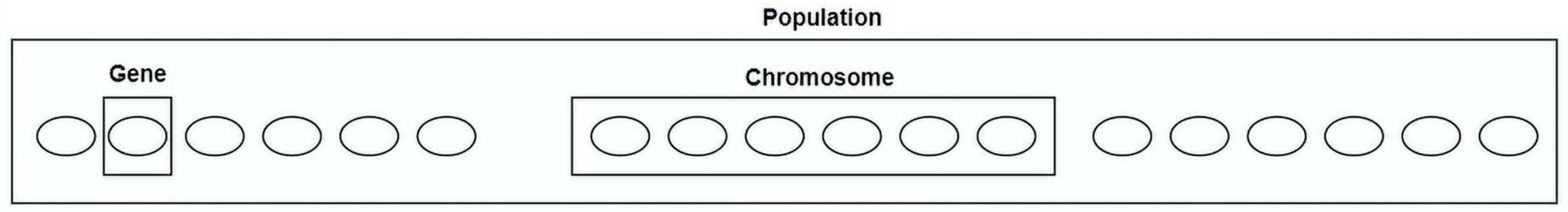
Genetic algorithms [14] are a heuristic search method inspired by biological evolution. As it is shown in Fig. 1, a possible solution to a given problem is coded as a chromosome, which is a sequence of genes that have certain values. For instance, if the problem is to find the shortest route that connects n cities, a chromosome could be used that consists of n genes where each gene refers to one of the n cities. A genetic algorithm operates on a set of chromosomes (hence on a set of possible solutions), where such a set is called a population. The initial population is composed of randomly generated chromosomes. Then, in an iterative process, subsequent generations are generated through operations called mutation and crossover and through fitness-oriented selection of the best chromosomes found so far. Mutation and crossover are applied on the selected chromosomes to create new chromosomes to be contained in the next generation. Various variants of mutation and crossover have been described in the literature (e.g. see [41]).
Figure 1.
An example of a simple population composed of three chromosomes, each consisting of six genes.
Genetic algorithm is used in varied fields. For instance, Thammasiri et al. [27] used 30 individual classifiers and encoded them to a binary chromosome (0: classifier not selected, 1: classifier selected). Finally, it used majority voting on the selected classifiers of the genetic algorithm for the final decision. Canuto et al. [17] proposed a genetic-based approach to select the best set of meta-features in the ensemble system.
3.Proposed method: MEGA
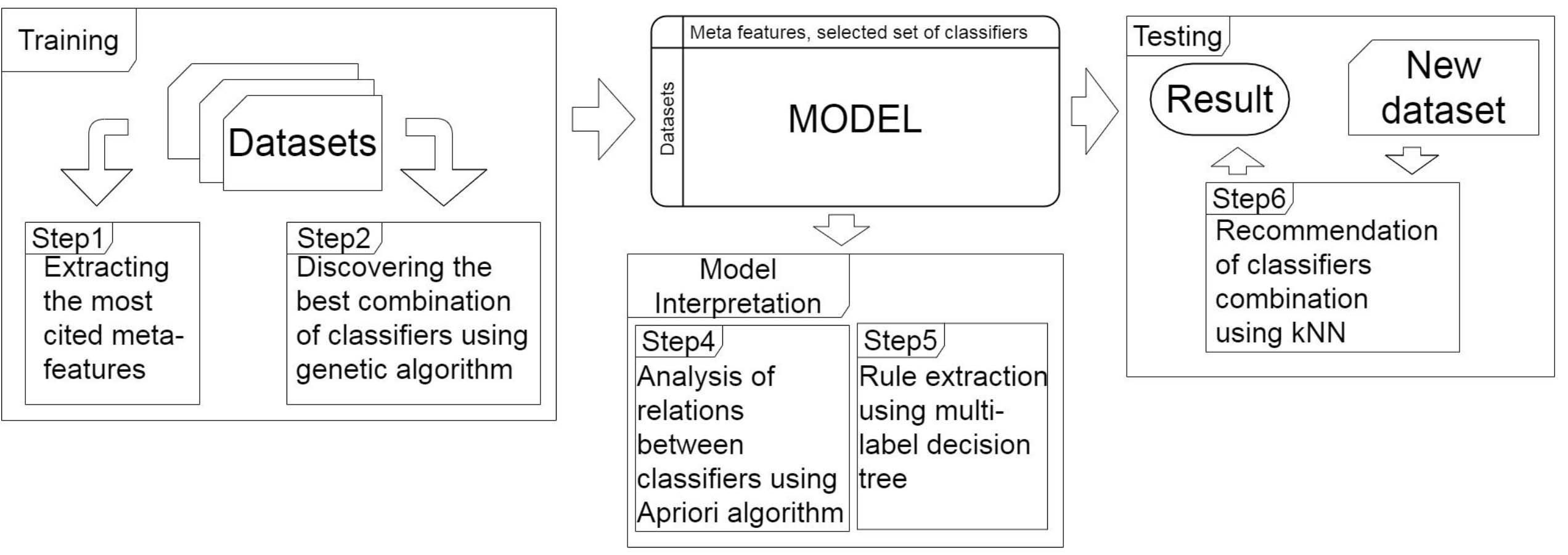
MEGA has three main components: a Training component, a Model Interpretation component and a Testing component. Figure 2 gives an overview of MEGA, including its three components and the main steps they are responsible for. We discuss each of the components in details in the following subsections.
Figure 2.
Overview of MEGA and the main steps executed by its three components. The Training component generates a model from meta-features by applying a genetic algorithm on input datasets. The Model Interpretation component interprets the generated model using a multi-label decision tree and an a priori algorithm. The Testing component recommends a combination of classifiers for an unseen dataset using kNN algorithm.
3.1Training component
The main input of MEGA is given by different datasets. If
Table 1
Set of meta-features in addition to A) list of citations and B) meta-feature group
| # | Meta-features | Group | Citation |
|---|---|---|---|
| 1 | Number of samples | General | [16, 24, 29, 30, 33, 10, 40, 42, 30] |
| [43, 44, 45, 46, 6, 47, 48, 35] | |||
| 2 | Number of classes | [16, 24, 29, 30, 40, 33, 10, 48, 42] | |
| [35, 43, 49, 45, 44, 46, 6, 47] | |||
| 3 | Number of features | [7, 6, 16, 29, 35, 40, 33, 47, 10] | |
| [48, 42, 43, 24, 45, 49, 44, 50] | |||
| 4 | Number of categorical features | [7, 16, 24, 6, 29, 35, 40, 33, 47] | |
| [10, 48, 42, 30, 44, 45, 50] | |||
| 5 | Number of numerical features | [7, 16, 24, 40, 42, 47, 10, 30] | |
| 6 | Dimension | [7, 29, 35, 10, 42, 43, 40, 46] | |
| 7 | Number of missing values | [16, 6, 30, 10, 48, 42, 24, 30] | |
| 8 | Proportion of missing values | [16, 6, 30, 10, 48, 42, 24, 30] | |
| 9 | Number of lines with missing value | [16, 6, 48, 24] | |
| 10 | Proportion of lines with missing value | [16, 6, 24] | |
| 11 | Number of data with noise | [16, 6, 24] | |
| 12 | Mean coefficient | Statistical | [29, 35, 43] |
| 13 | Max coefficient | [29, 35, 43] | |
| 14 | Min coefficient | [29, 35, 43] | |
| 15 | Mean covariance | [7, 48, 49] | |
| 16 | Max covariance | [7, 48, 49] | |
| 17 | Min covariance | [7, 48, 49] | |
| 18 | Mean of mean | [11, 10, 42, 45] | |
| 19 | Max of mean | [11, 10] | |
| 20 | Min of mean | [11, 10] | |
| 21 | Mean STD | [11, 10] | |
| 22 | Max STD | [11, 10] | |
| 23 | Min STD | [11, 10] | |
| 24 | Mean skewness | [11, 10] | |
| 25 | Max skewness | [11, 10] | |
| 26 | Min skewness | [11, 10] | |
| 27 | Mean kurtosis | [11, 10] | |
| 28 | Max kurtosis | [11, 10] | |
| 29 | Min kurtosis | [11, 10] | |
| 30 | Max attribute entropy | Informative | [11, 10] |
| 31 | Min attribute entropy | [10, 43] | |
| 32 | Mean attribute entropy | [29, 33, 11, 40, 16, 24, 6, 42, 43] | |
| [7, 10, 49, 45, 48, 35] | |||
| 33 | Mean mutual information | [7, 6, 29, 30, 43, 40, 11, 33, 49] | |
| [10, 35, 48, 42, 30, 24, 16, 45] | |||
| 34 | Class entropy | [49, 44, 7, 16, 24, 6, 29, 35, 40] | |
| [11, 33, 10, 49, 48, 42, 43, 45] |
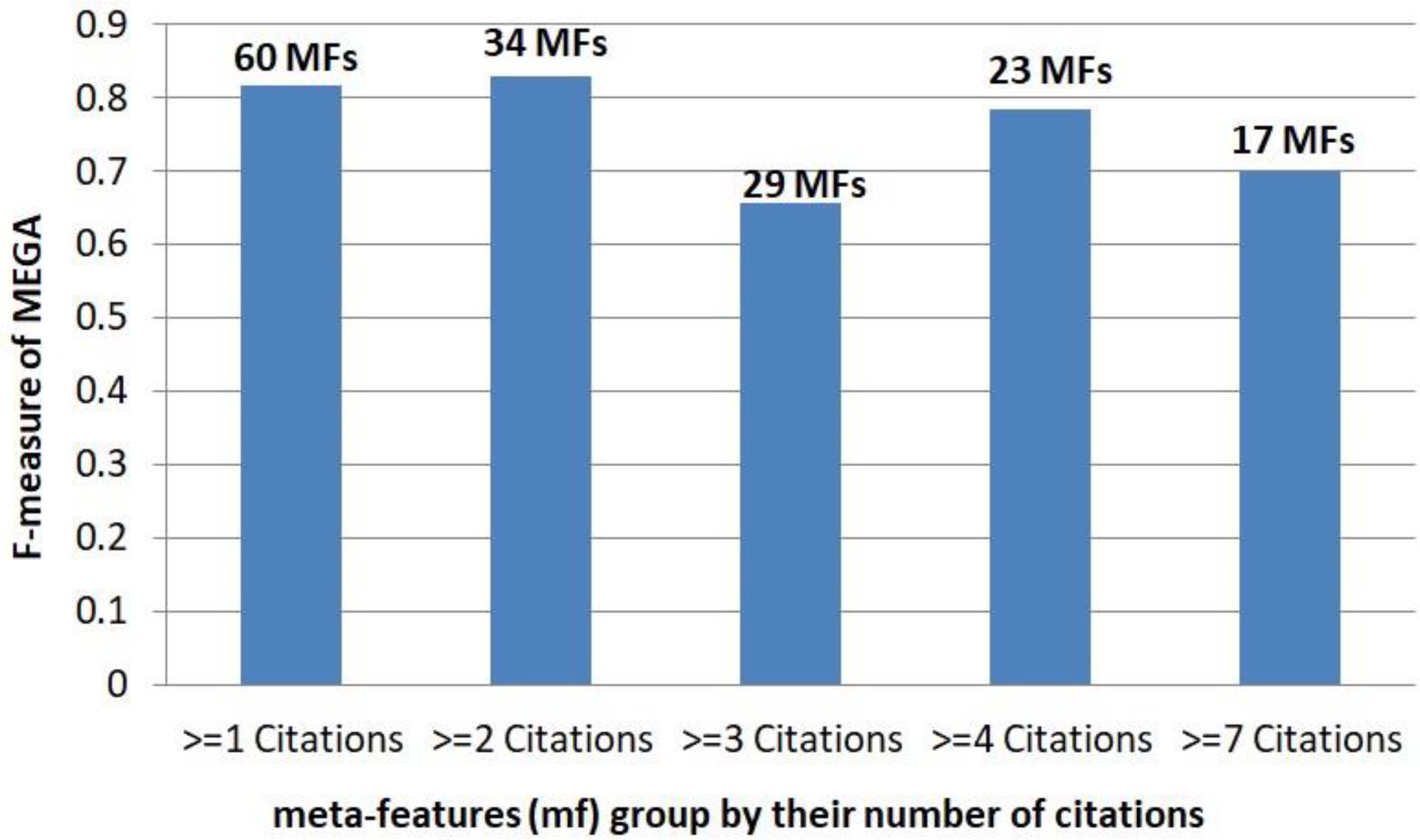
Figure 3.
The comparison of MEGA performance with a different subset of meta-features (mf) based on their number of citations. The performance of MEGA is the best among others when meta-features with at-least two publications are used as the set of meta-features.
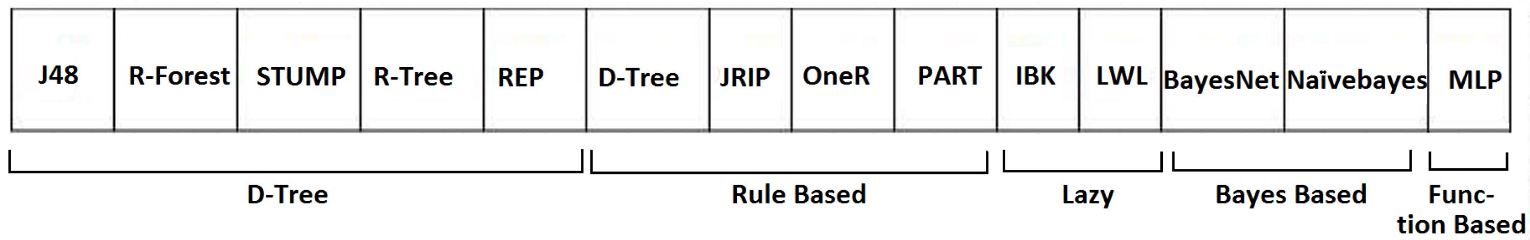
MEGA uses 14 initial classifiers: J48, Random forest, Stump, Random tree, REP, Decision table, JRIP, OneR, PART, IBk, LWL, Bayes net, Naive Bayes and MLP. Table 2 shows these 14 initial classifiers, their families (according to Weka [32] family categorization) and publications cited them in the ensemble systems and meta-learning fields. As it is shown in Table 2, Naive Bayes, MLP and JRIP are the most cited classifiers in the literature. Moreover, in order to discover the best combination of classifiers, MEGA uses a genetic algorithm, in which each gene is the binary representation of 14 individual classifiers existence in the recommended combination (1 means this individual classifier is in the combination and 0 means it is not). Figure 4 shows the chromosome and genes of the genetic algorithm, which is partitioned into the following five groups according to the five classifier families: 1) decision tree, 2) rule based, 3) lazy, 4) bayes based and 5) function based classifiers. After applying the genetic algorithm, MEGA represents the best found combination of classifiers for each dataset
Figure 4.
The chromosome of each individual as used by the genetic algorithm. It is partitioned into five classifier families, including Decision tree, Rule based, Lazy, Bayes based and Function based. Each gene expresses whether or not the respective individual classifier is part of the classifier combination.
The Training component concatenates two one-dimensional vectors,
Figure 5.
The matrix model MFBCC. The model establishes relationships between meta-features and classifier combinations for the training datasets
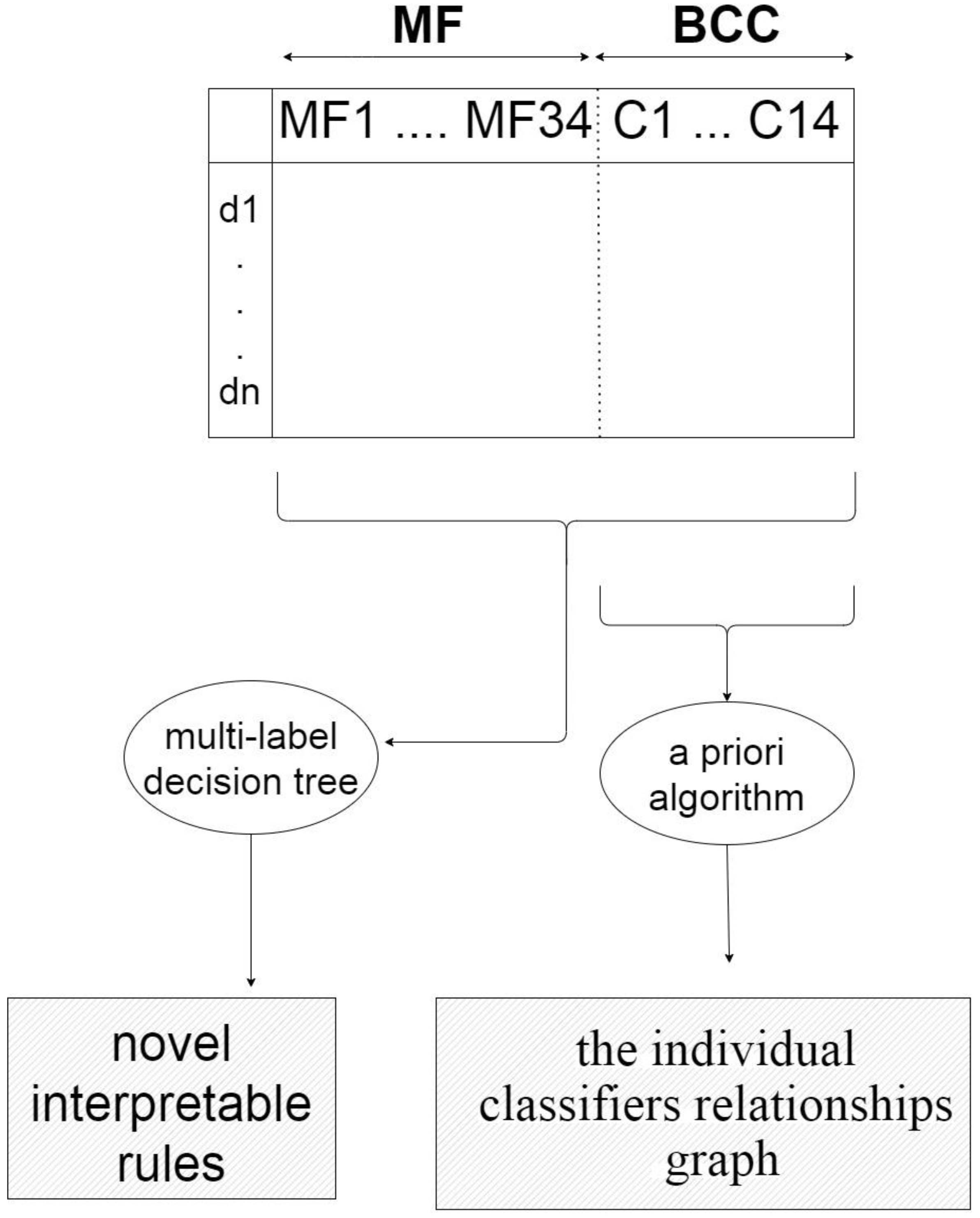
Table 2
The 14 selected classifiers, the families to which they below, publications citing them, and number of citations
| # | Classifier | Family | Citation | Citation count |
|---|---|---|---|---|
| 1 | J48 | Decision tree | [17, 51, 6, 52, 53, 47] | 6 |
| 2 | REP | [17, 51, 6, 53] | 4 | |
| 3 | Stump | [17, 34, 54, 6, 37] | 5 | |
| 4 | Random tree | [51] | 1 | |
| 5 | Random forest | [34, 52, 54, 47, 40] | 5 | |
| 6 | JRIP | Rule based | [6, 51, 10, 42, 55, 56, 34, 48, 57, 53, 30] | 11 |
| 7 | OneR | [17, 48, 40] | 3 | |
| 8 | PART | [17, 29, 51, 53, 6, 43] | 6 | |
| 9 | Decision table | [17, 6] | 2 | |
| 10 | Naive Bayes | Bayes | [7, 17, 29, 47, 16], | 25 |
| [43, 51, 37, 40, 51, 53], | ||||
| [58, 10, 48, 57, 47], | ||||
| [42, 30, 55, 24, 15, 59], | ||||
| [6, 60, 54] | ||||
| 11 | Bayes net | [34, 51, 53, 29, 43, 47] | 6 | |
| 12 | kNN | Lazy | [29, 48, 20, 42, 55, 43, 56, 51] | 8 |
| 13 | LWL | [42, 30] | 2 | |
| 14 | MLP | Function | [16, 24, 37, 40, 33, 53, 30, 55, 60], | 14 |
| [17, 48, 56, 59, 52] |
3.1.1Model interpretation component
This component is responsible for interpreting the matrix
• First, MEGA applies an a priori algorithm [61] to the BCC part of
The applied a priori algorithm is a frequent item sets mining algorithm, which has two main measures, named support and confidence [61, 62, 63, 64]. The support is the probability of transactions that contain both A and B (
• Next, MEGA applies multi-label learning and, specifically, uses MEKA [66] to generate a multi-label decision tree that allows to identify novel interpretable rules for recommending a useful combination of classifiers for an unseen dataset on the basis of its meta-features. Instead of just one label, the Multi-label learning approach predicts a set of labels (the existence of individual classifiers in an ensemble system) for each example (a given problem) [67, 68, 69]. For illustration, as it is indicated in Table 4 and will be discussed in details in Section 4.2.1, in dataset cases where the class entropy meta-feature is more than a threshold, then J48 classifier is recommended to be part of classifier combination in an ensemble system. In other words, class entropy and number of outliers meta-features describe the situations where J48 classifier suits best in ensemble systems.
3.2Testing component
The main task of this component is to predict the set of classifiers for a new dataset
(1)
where
4.Empirical results
In the following, we first introduce our datasets and then we discuss the results of the Training, Model Interpretation and Testing components of MEGA.
4.1Results of the training component
In this subsection, we introduce our selected set of training datasets and describe the configuration of the genetic algorithm used for discovering the best combination of classifiers for each training dataset.
4.1.1Training datasets
Table 3 shows 50 training UCI datasets [70] that are used in at least one of the previous methods discussed in Section 2 (together with their values of three fundamental meta-features “Number of classes”, “Type of features” and “Number of features”). These datasets are related to a number of subjects, including economics, medicine and politics, among others.
Table 3
50 UCI datasets and their characterization in terms of the meta-features “number of features”, “type of features” and “number of classes”
| # | Dataset name | Number of classes | Type of features | Number of features |
|---|---|---|---|---|
| 1 | Audit [71] | 2 | Numerical | 27 |
| 2 | Autism [72] | 2 | Categorical | 20 |
| 3 | Audiology [73] | 24 | Categorical | 69 |
| 4 | Balloons [74] | 2 | Categorical | 4 |
| 5 | Lung-cancer [75] | 3 | Categorical | 56 |
| 6 | Waveform | 3 | Numerical | 40 |
| 7 | kr-vs-kp [77] | 2 | Categorical | 36 |
| 8 | Banknote [78] | 2 | Numerical | 4 |
| 9 | Soybean-large [79] | 19 | Categorical | 35 |
| 10 | Caesarian [80] | 2 | Mix | 6 |
| 11 | Data-User-Modeling [81] | 4 | Numerical | 5 |
| 12 | Wpbc [82] | 2 | Numerical | 33 |
| 13 | Yeast [83] | 2 | Numerical | 3 |
| 14 | Wdbc [84] | 2 | Numerical | 30 |
| 15 | Diagnosis [85] | 2 | Mix | 7 |
| 16 | Fertility [69] | 2 | Numerical | 9 |
| 17 | Hayes-roth [86] | 3 | Categorical | 5 |
| 18 | Mushroom [87] | 2 | Categorical | 22 |
| 19 | Parkinsons [88] | 2 | Numerical | 22 |
| 20 | Healthy [89] | 4 | Numerical | 8 |
| 21 | Bank-additional [90] | 2 | Mix | 20 |
| 22 | AU [91] | 2 | Numerical | 20 |
| 23 | ILPD [92] | 2 | Mix | 10 |
| 24 | Magic04 [93] | 2 | Numerical | 10 |
| 25 | Lymphography [94] | 4 | Categorical | 18 |
| 26 | Lenses [95] | 3 | Categorical | 4 |
| 27 | Primary-tumor [96] | 22 | Categorical | 17 |
| 28 | Mammography [97] | 2 | Numerical | 5 |
| 29 | Pendigits [98] | 10 | Numerical | 16 |
| 30 | Nursery [99] | 4 | Categorical | 8 |
| 31 | Bridges1 [100] | 6 | Mix | 11 |
| 32 | Phishing [101] | 2 | Categorical | 30 |
| 33 | Cmc [102] | 3 | Mix | 9 |
| 34 | Monks-1 [103] | 2 | Categorical | 9 |
| 35 | Qualitative [70] | 2 | Categorical | 6 |
| 36 | Cervical-cancer [104] | 2 | Mix | 36 |
| 37 | HTRU [105] | 28 | Mix | 8 |
| 38 | Abalone [106] | 2 | Mix | 8 |
| 39 | Spam-base [70] | 2 | Numerical | 57 |
| 40 | Post-operative [107] | 3 | Mix | 8 |
| 41 | Transfusion [108] | 8 | Numerical | 7 |
| 42 | Tae [109] | 3 | Numerical | 5 |
| 43 | Thoraric-surgery [110] | 2 | Mix | 16 |
| 44 | Tic-tac-toe [111] | 2 | Categorical | 6 |
| 45 | Shuttle-landing [112] | 2 | Categorical | 6 |
| 46 | Wilt [113] | 2 | Numerical | 5 |
| 47 | Wifi [114] | 4 | Numerical | 7 |
| 48 | Avila [115] | 12 | Numerical | 10 |
| 49 | Wine [116] | 3 | Numerical | 12 |
| 50 | Trains [117] | 2 | Categorical | 3 |
Table 4
The most important rules generated by MEKA that relate the meta-features to the combination of classifiers. As can be seen from this table, these extracted rules use 21 of the 34 selected meta-features (“class entropy”, “number of outliers”, and so forth)
| Name | Rule |
|---|---|
| Rule1 | If “the class entropy” is smaller than 0.99656 and “the number of outliers” is smaller than 0.211099 and “the number of categorical attribute” is more than 0.219178, and “the minimum kurtosis” is smaller or equal to 0.381247 then J48 is recommended. |
| Rule2 | If “the class entropy” is smaller than 0.99656 and “the number of outliers” is more than 0.211099 then J48 is recommended. |
| Rule3 | If “the feature type” is numerical and “the number of outliers” is more than 0.019367 then Random Forest is recommended. |
| Rule4 | If ‘the number of attributes” is equal or smaller than 0.01087 and “the number of examples“ is equal or smaller than 0.005003 then Decision Stump is recommended. |
| Rule5 | If “the maximum kurtosis” is equal to or smaller than 0.244191 and “the mean attribute correlation” is more than 0.576604 then REP is recommended. |
| Rule6 | If “the dimension” is equal to or smaller than 0.000009 and “the maximum STD” is equal to or smaller than 0.000017 and “the mean STD” is more than 0.000013 then JRIP is recommended. |
| Rule7 | If “the dimension” is equal to or smaller than 0.000009 and “the maximum STD” is equal to or smaller than 0.000017 and “the mean STD” is equal to or smaller than 0.000013 and “the mean coefficient” is equal to or smaller than 0.046832 and “the maximum coefficient” is more than 0.000253 then JRIP is recommended. |
| Rule8 | If “the dimension” is equal to or smaller than 0.000009 and “the maximum STD” is equal to or smaller than 0.000017 and “the mean STD” is equal to or smaller than 0.000013 and “the mean coefficient” is equal to or smaller than 0.046832 and “the maximum coefficient” is equal to or smaller than 0.000253 and “the mean mutual information” is equal to or smaller than 0.065948 and “the minimum mean” is equal to or smaller than 0.533838 then JRIP is recommended. |
| Rule9 | If “the maximum STD” is equal to or smaller than 0.000017, and “the mean STD” is equal to or smaller than 0.000013 and “the minimum kurtosis” is equal to or smaller than 0.175639 then IBk is recommended. |
| Rule10 | If “the maximum STD” is equal to or smaller than 0.000017, and “the mean STD” is equal to or smaller than 0.000013 and “the minimum kurtosis” is more than 0.175639 and “the mean skewness” is more than 0.298774 then IBk is recommended. |
| Rule11 | If “the relative outliers” is more than 0.070805 and “the number of attributes” is equal to or smaller than 0.033981 then Bayesnet is recommended. |
| Rule12 | If “the dimension” is equal to or smaller than 0.000009 and “the number of classes” is more than 0.153846 then Naive Bayes is recommended. |
| Rule13 | If “the mean STD” is equal to or smaller than 0.000013 and “the maximum mean” is equal to or smaller than 0.00006 and “the minimum kurtosis” is more than 0.570324, then MLP is recommended. |
| Rule14 | If “the mean STD” is equal to or smaller than 0.000013 and “the maximum mean” is equal to or smaller than 0.00006 and “the minimum kurtosis” is equal to or smaller than 0.570324 and “the minimum coefficient” is equal to or smaller than 0.997901 and more than 0.59512 and “the minimum mutual information” is equal to or smaller than 0.03498 then MLP is recommended. |
4.1.2Model (MFBCC) generation using a genetic algorithm
The
• First, for each
• Second, tuning the hyperparameters for each classifier is interesting and still very challenging task. The optimal value for hyperparameters of each classifier may be different from one dataset to another. As a result we use the default hyperparameters of each classifier in WEKA/MEKA.
• Third, to discover the best combination of classifiers, the genetic algorithm (i) uses an initial population of 1000 with a generation of 100. Each chromosome of the population has the structure shown in Fig. 4, (ii) applies single-point crossover with probability 0.6, (iii) applies bit-string mutation with probability 0.05, and (iv) finally combines the selected individual classifiers by simple majority voting.
4.2Results of the model interpretation component
This subsection describes the interpretation of the
4.2.1Using a multi-label decision tree to extract novel interpretable rules from the MFBCC model
As described above, MEGA reduces the task of predicting the best classifier combination to a multi-label classification task. For this purpose, MEKA [66], uses N binary classifiers for multi-label classification with N labels. Because of the MEKA’s [66] configurations, each extracted rule from MEKA [66] indicates the existence of only one individual classifier. After computing meta-features of each dataset, in order to discover the existence of each individual classifier in the best combination, the set of meta-features must be compared to the “if part” of each extracted rule. Table 4 shows rules generated by MEKA.
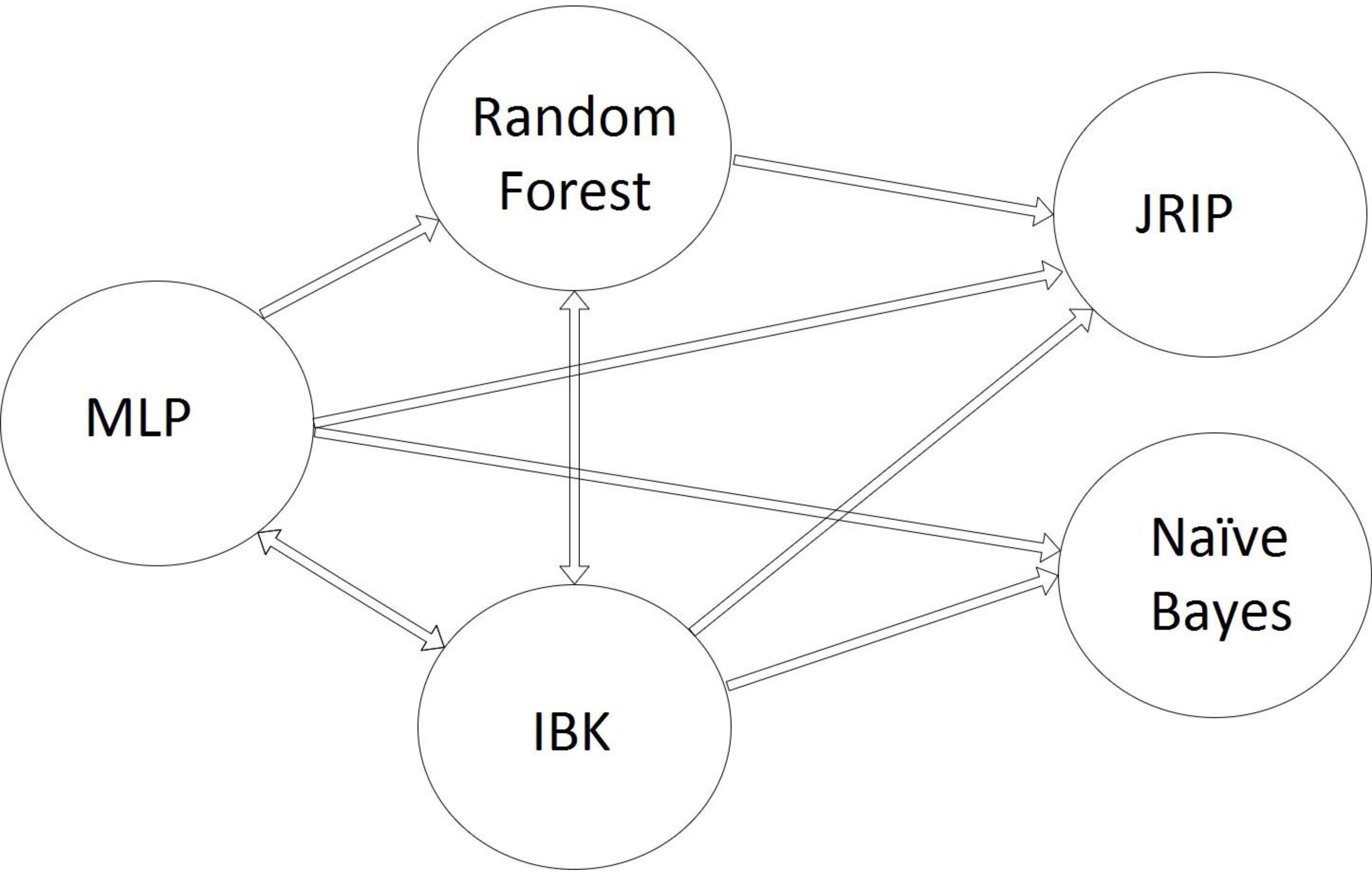
4.2.2Using an a priori algorithm to discover relations among individual classifiers
The BCC part of
• Each node belongs to one of the classifier families indicated in Table 2 and accordingly, the diversity of classifiers in the proposed ensemble is guaranteed.
• IBK classifier with the highest degree (with in-degree
• The cluster classifiers of MLP, Random forest and IBK, are the best set of classifier combinations in ensemble systems. They complement each other in varied perspectives, guaranty more variety in ensemble systems and explore more hypothesis spaces. Additionally, from interpretability point of view, MLP and Random forest are in complete opposite of each other. The results of MLP are more like black-box and Random forest produces easily interpretable results.
Figure 6.
Graph of relationships among the individual classifiers. Each node represents individual classifiers and each edge is the co-occurrence of individual classifiers in the best combination of classifiers.
![Comparison of MEGA and three other standard approaches [16, 7, 17] with respect to the F-measure.](https://content.iospress.com:443/media/ida/2021/25-6/ida-25-6-ida205494/ida-25-ida205494-g007.jpg)
4.3Results of the testing component
As described in Section 2.2, MEGA belongs to G2, that is, the group of meta-learning approaches that aim at combining classifiers. In the following, we present experimental results that compare MEGA with three other established methods from G2, namely, Neto et al. [7], Canuto et al. [17] and Nascimento et al. [16], where the method by Nascimento et al. allows for three variants (kNN, SVM and MLP). For the purpose of a sound comparison, we applied MEGA on the test datasets from these methods as the respective test phase of MEGA. Figure 7 shows the average F-measure of MEGA compared to the mentioned three methods. As it is shown, MEGA succeeded to increase the total average F-measure from 83% to 87%, compared to other methods. This means that MEGA achieves superior results and additionally is able to detect interpretable rules for combining classifiers. This is particularly remarkable because, to the best of our knowledge, there is no other method in G2 offering this desirable ability. It is desirable because it makes the achieved classification human-understandable.
5.Conclusions and future work
Classifier combination is one of the most effective methods for improving the performance of classifications. The most important issue for classifier selection apparently is the selection of the most suitable set of individual classifiers that should be combined. Because of the variety of individual classifiers, this selection can be extremely time-consuming. In this paper, we proposed MEGA, a novel method for classifier combination that exploits meta-learning and genetic algorithms and is composed of components for Training, Model Interpretation and Testing.
Comparing to previous work, the main contributions of MEGA are: (i) Varied range of meta-features and individual classifiers, (ii) automatic guarantee of diversity in the ensemble system and (iii) novel interpretable rules. Numerically, MEGA generates superior results comparing to three methods.
MEGA does not only achieve superior classification results compared to existing methods, but is also able to generate novel, human-interpretable classification rules. This “interpretability feature” makes MEGA particularly valuable for applications in domains (e.g., in the medical sector) that require explainable classification results, be it for legal or ethical reasons. Apart from this, MEGA is unique in that it additionally ensures diversity in the ensemble system and variability of the meta-features as well as the individual classifiers.
MEGA opens several promising avenues for future research. Among them is the exploration of other ensemble architectures such as bagging, boosting and multi-boosting, which can improve the performance of the result combination. As it is known genetic algorithm is an evolutionary algorithm, which its performance and the final result might be differ from one set of configuration to another. So, another avenue worth to investigate concerns the configuration of the genetic algorithm, possibly using different fitness functions such as accuracy and logarithmic loss, among others. A third promising avenue is using different meta-learners, such as SVM and different searching algorithm for finding the best combination of classifier in place of the genetic algorithm.
References
[1] | S.B. Kotsiantis, I. Zaharakis and P. Pintelas, Supervised machine learning: A review of classification techniques, Emerging Artificial Intelligence Applications in Computer Engineering 160: ((2007) ), 3–24. |
[2] | J.R. Rice, The algorithm selection problem, in: Advances in Computers, Elsevier, Vol. 15, (1976) , pp. 65–118. |
[3] | L.I. Kuncheva, Combining pattern classifiers: methods and algorithms, John Wiley & Sons, (2004) . |
[4] | T.G. Dietterich, Ensemble methods in machine learning, in: International Workshop on Multiple Classifier Systems, Springer, (2000) , pp. 1–15. |
[5] | G. Brown, Ensemble learning, in: Encyclopedia of Machine Learning, Springer, (2011) , pp. 312–320. |
[6] | R.R. Parente, A.M. Canuto and J.C. Xavier, Characterization measures of ensemble systems using a meta-learning approach, in: Neural Networks (IJCNN), The 2013 International Joint Conference on, IEEE, (2013) , pp. 1–8. |
[7] | A.A.F. Neto and A.M. Canuto, Meta-learning and multi-objective optimization to design ensemble of classifiers, in: Intelligent Systems (BRACIS), 2014 Brazilian Conference on, IEEE, (2014) , pp. 91–96. |
[8] | H. Guo, A bayesian approach for automatic algorithm selection, in: Proceedings of the International Joint Conference on Artificial Intelligence (IJCAI03), Workshop on AI and Autonomic Computing, Acapulco, Mexico, (2003) , pp. 1–5. |
[9] | J. Vanschoren, Meta-learning, in: Automated Machine Learning, Springer, (2019) , pp. 35–61. |
[10] | B. Bilalli, A. Abello and T. Aluja-Banet, On the predictive power of meta-features in openml, International Journal of Applied Mathematics and Computer Science 27: (4) ((2017) ), 697–712. |
[11] | M. Reif, F. Shafait and A. Dengel, Meta2-features: Providing meta-learners more information, in: 35th German Conference on Artificial Intelligence, Citeseer, (2012) , pp. 91–96. |
[12] | R. Vilalta, C. Giraud-Carrier and P. Brazdil, Meta-learning-concepts and techniques, in: Data Mining and Knowledge Discovery Handbook, Springer, (2009) , pp. 717–731. |
[13] | D. Whitley, A genetic algorithm tutorial, Statistics and Computing 4: (2) ((1994) ), 65–85. |
[14] | H. Holland John, Adaptation in natural and artificial systems, Ann Arbor: University of Michigan Press, (1975) . |
[15] | I. Tanfilev, A. Filchenkov and I. Smetannikov, Feature selection algorithm ensembling based on meta-learning, in: Image and Signal Processing, BioMedical Engineering and Informatics (CISP-BMEI), 2017 10th International Congress on, IEEE, (2017) , pp. 1–6. |
[16] | D.S. Nascimento, A.M. Canuto and A.L. Coelho, An empirical analysis of meta-learning for the automatic choice of architecture and components in ensemble systems, in: 2014 Brazilian Conference on Intelligent Systems (BRACIS), IEEE, (2014) , pp. 1–6. |
[17] | A.M. Canuto and D.S. Nascimento, A genetic-based approach to features selection for ensembles using a hybrid and adaptive fitness function, in: Neural Networks (IJCNN), The 2012 International Joint Conference on, IEEE, (2012) , pp. 1–8. |
[18] | L.I. Kuncheva and C.J. Whitaker, Measures of diversity in classifier ensembles and their relationship with the ensemble accuracy, Machine Learning 51: (2) ((2003) ), 181–207. |
[19] | L. Breiman, Bagging predictors, Machine Learning 24: (2) ((1996) ), 123–140. |
[20] | T.G. Dietterich, An experimental comparison of three methods for constructing ensembles of decision trees: Bagging, boosting, and randomization, Machine Learning 40: (2) ((2000) ), 139–157. |
[21] | D.S. Nascimento and A.L. Coelho, Ensembling heterogeneous learning models with boosting, in: International Conference on Neural Information Processing, Springer, (2009) , pp. 512–519. |
[22] | R.E. Schapire, The strength of weak learnability, Machine Learning 5: (2) ((1990) ), 197–227. |
[23] | Y. Freund, R.E. Schapire et al., Experiments with a new boosting algorithm, in: Icml, Citeseer, Vol. 96, (1996) , pp. 148–156. |
[24] | D. Nascimento, A. Canuto and A. Coelho, Multi-label meta-learning approach for the automatic configuration of classifier ensembles, Electronics Letters 52: (20) ((2016) ), 1688–1690. |
[25] | I. Webb, Idealized models of decision committee performance and their application to reduce committee error, Deakin University, School of Computing and Mathematics, (1998) . |
[26] | G.I. Webb, Multiboosting: A technique for combining boosting and wagging, Machine Learning 40: (2) ((2000) ), 159–196. |
[27] | D. Thammasiri and P. Meesad, Ensemble data classification based on diversity of classifiers optimized by genetic algorithm, in: Advanced Materials Research, Trans Tech Publ, Vol. 433, (2012) , pp. 6572–6578. |
[28] | A. Rivolli, L.P. Garcia, C. Soares, J. Vanschoren and A.C. de Carvalho, Towards reproducible empirical research in meta-learning, arXiv preprint arXiv:1808.10406, (2018) . |
[29] | A. Filchenkov and A. Pendryak, Datasets meta-feature description for recommending feature selection algorithm, in: Artificial Intelligence and Natural Language and Information Extraction, Social Media and Web Search FRUCT Conference (AINL-ISMW FRUCT), 2015, IEEE, (2015) , pp. 11–18. |
[30] | P.B. Brazdil, C. Soares and J.P. Da Costa, Ranking learning algorithms: Using ibl and meta-learning on accuracy and time results, Machine Learning 50: (3) ((2003) ), 251–277. |
[31] | S.Y. Sohn, Meta analysis of classification algorithms for pattern recognition, IEEE Transactions on Pattern Analysis and Machine Intelligence 21: (11) ((1999) ), 1137–1144. |
[32] | M. Hall, E. Frank, G. Holmes, B. Pfahringer, P. Reutemann and I.H. Witten, The weka data mining software: An update; sigkdd explorations, 2009, Software available at http://www.cs.waikato.ac.nz/ml/weka, (2009) . |
[33] | J. Gama and P. Brazdil, Characterization of classification algorithms, in: Portuguese Conference on Artificial Intelligence, Springer, (1995) , pp. 189–200. |
[34] | D. Garcia-Saiz and M. Zorrilla, Metalearning-based recommenders: towards automatic classification algorithm selection, expert systems, (2015) . |
[35] | C. Castiello, G. Castellano and A.M. Fanelli, Meta-data: Characterization of input features for meta-learning, in: International Conference on Modeling Decisions for Artificial Intelligence, Springer, (2005) , pp. 457–468. |
[36] | P. Brazdil, J. Gama and B. Henery, Characterizing the applicability of classification algorithms using meta-level learning, in: European Conference on Machine Learning, Springer, (1994) , pp. 83–102. |
[37] | M. Reif, A. Leveringhaus, F. Shafait and A. Dengel, Predicting classifier combinations, in: ICPRAM, (2013) , pp. 293–297. |
[38] | S. Ali and K.A. Smith, On learning algorithm selection for classification, Applied Soft Computing 6: (2) ((2006) ), 119–138. |
[39] | H. Bensusan and A. Kalousis, Estimating the predictive accuracy of a classifier, in: European Conference on Machine Learning, Springer, (2001) , pp. 25–36. |
[40] | M. Reif, F. Shafait, M. Goldstein, T. Breuel and A. Dengel, Automatic classifier selection for non-experts, Pattern Analysis and Applications 17: (1) ((2014) ), 83–96. |
[41] | H. Bhasin and S. Bhatia, Application of genetic algorithms in machine learning, IJCSIT 2: (5) ((2011) ), 2412–2415. |
[42] | A. Kalousis, Algorithm selection via meta-learning, Ph.D. dissertation, University of Geneva, (2002) . |
[43] | G. Wang, Q. Song, H. Sun, X. Zhang, B. Xu and Y. Zhou, A feature subset selection algorithm automatic recommendation method, Journal of Artificial Intelligence Research 47: ((2013) ), 1–34. |
[44] | C.K. Charles, C. Taylor and J. Keller, Meta-analysis: From data characterisation for meta-learning to meta-regression, in: Proceedings of the PKDD-00 Workshop on Data Mining, Decision Support, Meta-Learning and ILP, Citeseer, (2000) . |
[45] | M. Tripathy and A. Panda, A study of algorithm selection in data mining using meta-learning, Journal of Engineering Science & Technology Review 10: (2) ((2017) ). |
[46] | R.B. Prudencio, M.C. De Souto and T.B. Ludermir, Selecting machine learning algorithms using the ranking meta-learning approach, in: Meta-Learning in Computational Intelligence, Springer, (2011) , pp. 225–243. |
[47] | R. Espinosa, D. Garcia-Saiz, M.E. Zorrilla, J.J. Zubcoff and J.-N. Mazon, Development of a knowledge base for enabling non-expert users to apply data mining algorithms, in: SIMPDA, Citeseer, (2013) , pp. 46–61. |
[48] | G. Lindner and R. Studer, Ast: Support for algorithm selection with a cbr approach, in: European Conference on Principles of Data Mining and Knowledge Discovery, Springer, (1999) , pp. 418–423. |
[49] | K.A. Smith-Miles, Cross-disciplinary perspectives on meta-learning for algorithm selection, ACM Computing Surveys (CSUR) 41: (1) ((2009) ), 6. |
[50] | H. Bensusan, C. Giraud-Carrier and C.J. Kennedy, A higher-order approach to meta-learning, ILP Work-in-Progress Reports 35: ((2000) ). |
[51] | S. Alyahyan and W. Wang, Feature level ensemble method for classifying multi-media data, in: International Conference on Innovative Techniques and Applications of Artificial Intelligence, Springer, (2017) , pp. 235–249. |
[52] | M.A. Firdaus, R. Nadia and B.A. Tama, Detecting major disease in public hospital using ensemble techniques, in: Technology Management and Emerging Technologies (ISTMET), 2014 International Symposium on, IEEE, (2014) , pp. 149–152. |
[53] | M. Molina, J. Luna, C. Romero and S. Ventura, Meta-learning approach for automatic parameter tuning: A case study with educational datasets, International Educational Data Mining Society, (2012) . |
[54] | T. Horvath and J.M. Aldahdooh, Investigating the importance of meta-features for classification tasks in meta-learning, Ph.D. dissertation, Eötvös Loránd University, (2017) . |
[55] | H. Bensusan and C. Giraud-Carrier, Discovering task neighbourhoods through landmark learning performances, in: European Conference on Principles of Data Mining and Knowledge Discovery, Springer, (2000) , pp. 325–330. |
[56] | Y. Peng, P.A. Flach, C. Soares and P. Brazdil, Improved dataset characterisation for meta-learning, in: International Conference on Discovery Science, Springer, (2002) , pp. 141–152. |
[57] | B. Pfahringer, H. Bensusan and C.G. Giraud-Carrier, Meta-learning by landmarking various learning algorithms, in: ICML, (2000) , pp. 743–750. |
[58] | N. Jankowski, Graph-based generation of a meta-learning search space, International Journal of Applied Mathematics and Computer Science 22: (3) ((2012) ), 647–667. |
[59] | K. Gao, T.M. Khoshgoftaar and R. Wald, Combining feature selection and ensemble learning for software quality estimation, in: FLAIRS Conference, (2014) . |
[60] | G. Nakhaeizadeh and A. Schnabl, Development of multi-criteria metrics for evaluation of data mining algorithms, in: KDD, (1997) , pp. 37–42. |
[61] | S. Kotsiantis and D. Kanellopoulos, Association rules mining: A recent overview, GESTS International Transactions on Computer Science and Engineering 32: (1) ((2006) ), 71–82. |
[62] | K. Lai and N. Cerpa, Support vs. confidence in association rule algorithms, in: Proceedings of the OPTIMA Conference, Curicó, (2001) , pp. 1–14. |
[63] | P. Fournier-Viger, J.C.-W. Lin, R.U. Kiran, Y.S. Koh and R. Thomas, A survey of sequential pattern mining, Data Science and Pattern Recognition 1: (1) ((2017) ), 54–77. |
[64] | B. Goethals and M.J. Zaki, Advances in frequent itemset mining implementations: Report on fimi’03, SIGKDD Explorations 6: (1) ((2004) ), 109–117. |
[65] | R. Agrawal, T. Imieliński and A. Swami, Mining association rules between sets of items in large databases, in: Acm Sigmod Record, ACM, Vol. 22, No. 2, (1993) , pp. 207–216. |
[66] | J. Read, P. Reutemann, B. Pfahringer and G. Holmes, MEKA: A multi-label/multi-target extension to Weka, Journal of Machine Learning Research 17: (21) ((2016) ), 1–5. [Online]. Available: http://jmlr.org/papers/v17/12-164.html. |
[67] | M.-L. Zhang and Z.-H. Zhou, A review on multi-label learning algorithms, IEEE Transactions on Knowledge and Data Engineering 26: (8) ((2013) ), 1819–1837. |
[68] | G. Tsoumakas, E. Spyromitros-Xioufis, J. Vilcek and I. Vlahavas, Mulan: A java library for multi-label learning, Journal of Machine Learning Research 12: (Jul) ((2011) ), 2411–2414. |
[69] | E. Gibaja and S. Ventura, A tutorial on multilabel learning, ACM Computing Surveys (CSUR) 47: (3) ((2015) ), 52. |
[70] | D. Dheeru and E. Karra Taniskidou, Uci machine learning repository, (2017) . [Online]. Available: http://archive.ics.uci.edu/ml. |
[71] | N. Hooda, S. Bawa and P.S. Rana, Fraudulent firm classification: A case study of an external audit, Applied Artificial Intelligence 32: (1) ((2018) ), 48–64. |
[72] | F. Thabtah, Autism spectrum disorder screening: machine learning adaptation and dsm-5 fulfillment, in: Proceedings of the 1st International Conference on Medical and Health Informatics 2017, ACM, (2017) , pp. 1–6. |
[73] | Jergen, Standardized audiology database, (1987) , http://archive.ics.uci.edu/ml/datasets/audiology+(standardized). |
[74] | M.J. Pazzani, Influence of prior knowledge on concept acquisition: Experimental and computational results, Journal of Experimental Psychology: Learning, Memory, and Cognition 17: (3) ((1991) ), 416. |
[75] | Z.-Q. Hong and J.-Y. Yang, Lung cancer data, (1991) , https://archive.ics.uci.edu/ml/datasets/lung+cancer. |
[76] | L. Breiman, J.H. Friedman, A. Olshen and J. Stone, Waveform database generator, (1984) , https://archive.ics.uci.edu/ml/machine-learning-databases/waveform. |
[77] | A. Shapiro, Chess end-game – king+rook versus king+pawn on a7, (1989) , https://archive.ics.uci.edu/ml/datasets/Chess+(King-Rook+vs.+King-Pawn). |
[78] | J.R. Quinlan, Credit approval, (1987) , https://archive.ics.uci.edu/ml/datasets/credit+approval. |
[79] | R.S. Michalski and R. Chilausky, Large soybean database, (1988) , https://archive.ics.uci.edu/ml/datasets/Soybean+(Large). |
[80] | M. Amin and A. Ali, Performance evaluation of supervised machine learning classifiers for predicting healthcare operational decisions, Wavy AI Research Foundation: Lahore, Pakistan, (2018) . |
[81] | H.T. Kahraman, S. Sagiroglu and I. Colak, The development of intuitive knowledge classifier and the modeling of domain dependent data, Knowledge-Based Systems 37: ((2013) ), 283–295. |
[82] | W. Wolberg, N. Street and O. Mangasarian, Wisconsin prognostic breast cancer (wpbc), (1995) , https://archive.ics.uci.edu/ml/datasets/Breast+Cancer+Wisconsin+(Prognostic). |
[83] | K. Nakai, Protein localization sites, (1996) , https://archive.ics.uci.edu/ml/datasets/ecoli. |
[84] | W. Wolberg, N. Street and O. Mangasarian, Wisconsin diagnostic breast cancer (wdbc), (1993) , https://archive.ics.uci.edu/ml/datasets/Breast+Cancer+Wisconsin+(Diagnostic). |
[85] | V. Lohweg, F. Paschke, C. Bayer, M. Bator, U. Mönks, A. Dicks and O. Enge-Rosenblatt, Sensorlose zustandsüberwachung an synchronmotoren. |
[86] | G. Melli, A Lazy Model-Based Approach to On-Line Classification, Citeseer, (1998) . |
[87] | A.A. Knopf, Mushroom, (1981) , https://archive.ics.uci.edu/ml/datasets/mushroom. |
[88] | M. Little, Parkinsons disease data set, (2007) , https://archive.ics.uci.edu/ml/datasets/parkinsons. |
[89] | R.L.S. Torres, D.C. Ranasinghe, Q. Shi and A.P. Sample, Sensor enabled wearable rfid technology for mitigating the risk of falls near beds, in: 2013 IEEE International Conference on RFID (RFID), IEEE, (2013) , pp. 191–198. |
[90] | S. Moro, P. Cortez and P. Rita, Bank marketing data set, (2014) , https://archive.ics.uci.edu/ml/datasets/bank+marketing. |
[91] | G.R. Marrs, R.J. Hickey and M. Black, Modeling the example life-cycle in an online classification learner, in: Online Proceedings of HaCDAIS 2010 (First International Workshop on Handling Concept Drift in Adaptive Information Systems), ECML/PKDD 2010, Online Proceedings of HaCDAIS 2010 (First International Workshop on Handling, (2010) . |
[92] | B.V. Ramana, M.S.P. Babu and N. Venkateswarlu, A critical comparative study of liver patients from usa and india: An exploratory analysis, International Journal of Computer Science Issues (IJCSI) 9: (3) ((2012) ), 506. |
[93] | G. Gong, Hepatitis domain, (1988) , https://archive.ics.uci.edu/ml/datasets/hepatitis. |
[94] | M. Zwitter and M. Soklic, Lymphography domain, (1988) , https://archive.ics.uci.edu/ml/datasets/Lymphography. |
[95] | B.A. MacDonald and I.H. Witten, Using concept learning for knowledge acquisition, (1987) . |
[96] | M. Zwitter and M. Soklic, Primary tumor data set, (1988) , https://archive.ics.uci.edu/ml/datasets/primary+tumor. |
[97] | M. Elter, R. Schulz-Wendtland and T. Wittenberg, The prediction of breast cancer biopsy outcomes using two cad approaches that both emphasize an intelligible decision process, Medical Physics 34: (11) ((2007) ), 4164–4172. |
[98] | F. Alimoglu and E. Alpaydin, Pen-based recognition of handwritten digits data set, (1996) , https://archive.ics.uci.edu/ml/datasets/Pen-Based+Recognition+of+Handwritten+Digits. |
[99] | M. Olave, V. Rajkovic and M. Bohanec, An application for admission in public school systems, Expert Systems in Public Administration 1: ((1989) ), 145–160. |
[100] | Y. Reich and S.J. Fenves, Pittsburgh bridges, (1990) , https://archive.ics.uci.edu/ml/datasets/Pittsburgh+Bridges. |
[101] | R.M. Mohammad, F. Thabtah and L. McCluskey, An assessment of features related to phishing websites using an automated technique, in: 2012 International Conference for Internet Technology and Secured Transactions, IEEE, (2012) , pp. 492–497. |
[102] | T.- Lim, Contraceptive method choice, (1987) , https://archive.ics.uci.edu/ml/datasets/Contraceptive+Method+Choice. |
[103] | S. Thrun, The monk’s problems, (1992) , https://archive.ics.uci.edu/ml/datasets/MONK’s+Problems. |
[104] | K. Fernandes, J.S. Cardoso and J. Fernandes, Transfer learning with partial observability applied to cervical cancer screening, in: Iberian Conference on Pattern Recognition and Image Analysis, Springer, (2017) , pp. 243–250. |
[105] | R. Lyon, Htru2, (2017) , https://archive.ics.uci.edu/ml/datasets/HTRU2. |
[106] | W.J. Nash, S.T.L, S.R. Talbot, A.J. Cawthorn and W.B. Ford, Abalone data, (1994) , https://archive.ics.uci.edu/ml/datasets/abalone. |
[107] | L. Woolery and S. Summers, Postoperative patient data, (1991) , https://archive.ics.uci.edu/ml/datasets/Post-Operative+Patient. |
[108] | I.-C. Yeh, K.-J. Yang and T.-M. Ting, Blood transfusion service center data set, (2008) , https://archive.ics.uci.edu/ml/datasets/Blood+Transfusion+Service+Center. |
[109] | W.-Y. Loh and Y.-S. Shih, Split selection methods for classification trees, Statistica sinica, (1997) , 815–840. |
[110] | M. Zikeba, J.M. Tomczak, M. Lubicz and J. Swikatek, Boosted svm for extracting rules from imbalanced data in application to prediction of the post-operative life expectancy in the lung cancer patients, Applied Soft Computing 14: ((2014) ), 99–108. |
[111] | D.W. Aha, Tic-tac-toe endgame database, (1990) , https://archive.ics.uci.edu/ml/datasets/Tic-Tac-Toe+Endgame. |
[112] | NASA, Shuttle landing control data set, (1988) , https://archive.ics.uci.edu/ml/datasets/Shuttle+Landing+Control. |
[113] | B. Johnson, R. Tateishi and N. Thanh Hoan, Wilt, (2013) , http://archive.ics.uci.edu/ml/datasets/wilt. |
[114] | J.G. Rohra, B. Perumal, S.J. Narayanan, P. Thakur and R.B. Bhatt, User localization in an indoor environment using fuzzy hybrid of particle swarm optimization & gravitational search algorithm with neural networks, in: Proceedings of Sixth International Conference on Soft Computing for Problem Solving, Springer, (2017) , pp. 286–295. |
[115] | R.S. Siegler, Balance scale weight & distance database, (1976) , http://archive.ics.uci.edu/ml/datasets/balance+scale. |
[116] | S. Aeberhard, D. Coomans and O. De Vel, Comparative analysis of statistical pattern recognition methods in high dimensional settings, Pattern Recognition 27: (8) ((1994) ), 1065–1077. |
[117] | R.S. Michalski and R. Stepp, Induce trains data set, (1994) , https://archive.ics.uci.edu/ml/datasets/Trains. |
[118] | L. Al Shalabi and Z. Shaaban, Normalization as a preprocessing engine for data mining and the approach of preference matrix, in: 2006 International Conference on Dependability of Computer Systems, IEEE, (2006) , pp. 207–214. |
[119] | J. Han, J. Pei and M. Kamber, Data mining: concepts and techniques, Elsevier, (2011) . |


