Railway alignment optimization in regions with densely-distributed obstacles based on semantic topological maps

Wan, Xinjie; Pu, Hao; Schonfeld, Paul; Song, Taoran; Li, Wei; Peng, Lihui

doi:10.3233/ICA-240739

Railway alignment optimization in regions with densely-distributed obstacles based on semantic topological maps

Article type: Research Article

Authors: Wan, Xinjie^{a; b} | Pu, Hao^{a; b; *} | Schonfeld, Paul^c | Song, Taoran^{a; b} | Li, Wei^{a; b} | Peng, Lihui^d

Affiliations: [a] School of Civil Engineering, Central South University, Changsha, Hunan, China | [b] National Engineering Research Center of High-speed Railway Construction Technology, Changsha, Hunan, China | [c] Department of Civil and Environmental Engineering, University of Maryland, College Park, MD, USA | [d] China Railway Siyuan Survey and Design Group Co. Ltd, Wuhan, Hubei, China

Correspondence: [*] Corresponding author: Hao Pu, National Engineering Research Center of High-speed Railway Construction Technology, Changsha 410075, Hunan, China. E-mail: [email protected].

Keywords: Railway design, alignment optimization, geographic analysis, constrained optimization, semantic topological map

DOI: 10.3233/ICA-240739

Journal: Integrated Computer-Aided Engineering, vol. Pre-press, no. Pre-press, pp. 1-17, 2024

Published: 9 April 2024

Get PDF

Abstract

Railway alignment development in a study area with densely-distributed obstacles, in which regions favorable for alignments are isolated (termed an isolated island effect, i.e., IIE), is a computation-intensive and time-consuming task. To enhance search efficiency and solution quality, an environmental suitability analysis is conducted to identify alignment-favorable regions (AFRs), focusing the subsequent alignment search on these areas. Firstly, a density-based clustering algorithm (DBSCAN) and a specific criterion are customized to distinguish AFR distribution patterns: continuously-distributed AFRs, obstructed effects, and IIEs. Secondly, a study area characterized by IIEs is represented with a semantic topological map (STM), integrating between-island and within-island paths. Specifically, between-island paths are derived through a multi-directional scanning strategy, while within-island paths are optimized using a Floyd-Warshall algorithm. To this end, the intricate alignment optimization problem is simplified into a shortest path problem, tackled with conventional shortest path algorithms (of which Dijkstra’s algorithm is adopted in this work). Lastly, the proposed method is applied to a real case in a mountainous region with karst landforms. Numerical results indicate its superior performance in both construction costs and environmental suitability compared to human designers and a prior alignment optimization method.

1.Introduction

Railway alignment design is a complicated process, which aims to determine the railway geometric profiles [1, 2] and structure configurations [3, 4] between two given points. This process takes into account various factors such as topographic [5, 6] and geologic [7] conditions, alongside numerous hard-to-quantify objectives [8, 9]. Currently, this iterative and time-consuming railway design process is still mainly conducted by human designers. However, due to finite time and resources, several promising alignment alternatives may still be overlooked, especially when alignment-favorable regions (AFRs) are sparse in the study area. Optimizing an alignment in such cases requires substantial time and effort. To enhance the alignment generation efficiency and solution quality, many computer-aided approaches have been proposed for automatically optimizing alignments between two given points [10, 11].

Alignment determination is inherently an optimization problem, comprising three essential components: objective functions, design variables and constraints. The objective function is a mathematical expression of alignment fitness in terms of various factors, such as construction costs, geologic and ecologic conditions [12]. An alignment is typically described as a sequence of points of intersection (PIs) and their corresponding curve sections [13]. Therefore, the geometric parameters of alignment PIs and curves are defined as the design variables [14]. Constraints are imposed for ensuring that alignments adhere to railway design criteria, construction limitations, and their relative positions to other ground features [15].

Most alignment optimization methods can be categorized into two main types: nature-inspired methods and shortest-path methods. These classifications are based on the evolutionary mechanism of the PIs.

(1) In nature-inspired alignment optimization methods, all PIs are generated at the initial stage and iteratively adjusted according to the alignment fitness, considering various costs and impacts. Once the iterative adjustment process converges, the selected PIs determine an optimized alignment. Several effective nature-inspired methods have been applied in optimizing highway and railway alignments, such as genetic algorithms (GA) [16, 17], particle swarm optimization (PSO) [18, 19] and ant colony optimization (ACO) [20, 21]. In addition, hybrid optimization methods that integrate two or more nature-inspired approaches, such as a GA-ACO [22] and a PSO-GA [23], have been proposed for outperforming non-hybrid methods in alignment optimization.
(2) Shortest-path alignment optimization methods involve selecting and accumulating the best PIs within local ranges to form a complete alignment. Various approaches have been used in shortest-path alignment optimization, including grid-based methods using distance transforms (DT) [24, 25], graph-based methods using Dijkstra’s algorithms [26, 27] and sampling-based methods using rapidly exploring random tree algorithms (RRT) [28, 29]. These methods have proven successful in solving alignment optimization problems.

In nature-inspired alignment optimization methods, the fixed number of PIs during the alignment search process limits their application in complex alignment design spaces. This rigidity arises from the need to adjust the number of PIs flexibly, particularly when navigating densely-distributed obstacles. On the other hand, shortest-path algorithms yield outcomes comprising piecewise line segments, necessitating further adjustments into a detailed alignment solution. This involves configuring curve sections and determining structure layouts, thereby deviating from the initially optimized path.

Given the limitations of these methods, researchers have sought to combine them to tackle alignment optimization problems in intricate study areas. Drawing inspiration from the area-corridor-alignment design philosophy employed by human designers, Li et al. [26] customized DT to generate paths, represented as piecewise line segments, during the area-corridor design stage. They then utilized a GA to refine the alignment alternatives in the corridor-alignment design stage. Furthermore, Karlson et al. [8] developed a bi-objective optimization model for railway corridor planning that accounted for ecologic and geologic factors. Mondal et al. [30] adopted a combination approach, utilizing a derivative-free optimization method (NOMAD) along with a parallel search package to generate horizontal alignments within a predefined corridor.

All the alignment optimization methods mentioned above are based on some iterative process, where constraints are checked and handled during the search process in which an alignment is deemed infeasible if it violates any considered constraints [31]. However, these methods face challenges in study areas with densely-distributed obstacles, where feasible alignment regions are significantly squeezed and fragmented by multiple obstacles. This results in inefficient exploration of alignment-unfavorable regions, consuming substantial computing resources and time.

Several obstacle preprocessing methods have been developed in the motion planning field to address these challenges. Li et al. [32] abstracted obstacles as hexagons, constructing a feasible path network by connecting selected vertexes from these hexagons. Paths were considered infeasible if the line connecting adjacent vertexes intersected obstacles. Hu et al. [33] developed a Voronoi Diagram (VD) based on obstacles and subsequent path optimization was applied to this VD. While these methods shed new light on obstacle handling strategies, generating satisfactory solutions in areas with densely-distributed obstacles remained challenging, particularly if all obstacles were treated as forbidden regions.

To address this problem, Pu et al. [34] have abstracted the study area as a grid set and performed environmental suitability evaluation on these grid cells. Afterward, the AFRs are identified, and the subsequent alignment search process focuses on these regions. In Pu et al. [34], a connecting patch of AFRs envelops the start and end points, creating a pattern characterized by continuously-distributed AFRs across the study area. In this case, the existing alignment optimization methods can efficiently produce optimized alignments with the assistance of the environmental suitability analysis [34].

As China’s railway construction environment grows increasingly complex and research progresses, the authors’ team has found that in regions characterized by undulating terrains, AFRs include obstructions such as high mountains or deep valleys [35]. This poses a significant challenge in devising optimized layouts for dominating structures (i.e., deep-buried long tunnels and large-span high bridges) using traditional alignment optimization methods. Thus, Wan et al. [35] developed a bi-level optimization model for determining dominating structures at the upper level and optimizing the complete alignments at the lower-level. According to the characteristics of the distribution pattern of AFRs, study areas with the above-mentioned conditions are referred to as obstructed effects in this paper.

In recent years, as China’s railway network continued to expand and improve, several real-world railway scenarios have presented substantial challenges to alignment design. For example, in a section of the Shanghai-Chongqing-Chengdu High-speed Railway, karst hazards dominate almost 90% of the study area. This widespread presence of geo-hazards, coupled with ecologically sensitive regions, creates an alignment search space densely packed with obstacles. Moreover, urban high-speed railways increasingly contend with complex networks, such as existing roads and rivers, along with planar constraints such as existing buildings and water conservation zones. These constraints result in severe fragmentation of feasible regions available for traversing alignments.

Given this landscape, existing computer-aided alignment optimization methods face considerable difficulties in efficiently generating satisfactory alignment solutions. Ensuring solution quality while accommodating numerous constraints becomes a daunting task within such intricate and constrained environments.

Given the increasing complexity of China’s railway construction environment and the prevalence of study areas with densely-distributed obstacles, there is a growing need to overcome the limitations imposed on alignment optimization efficiency and quality by IIEs. Consequently, this paper introduces a completely new alignment optimization framework tailored to address the intricate alignment optimization challenges encountered in study areas with IIEs. Notably, given the complexity of this challenge, this study primarily focuses on generating alignment corridor alternatives during the area-corridor design stage. These alternatives serve as initial optimized corridors for subsequent stages, particularly the corridor-alignment stage. It is important to highlight that while the existing alignment optimization methods can efficiently address the optimization problems at the corridor-alignment stage, this paper does not focus on this aspect.

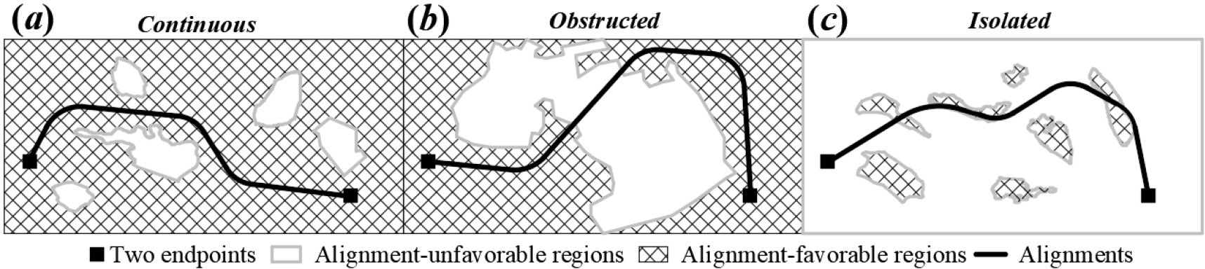
Figure 1.

Three different land parcel distribution patterns: AFRs are (a) continuous; (b) obstructed and (c) isolated.

The main contributions of this work are summarized as follows:

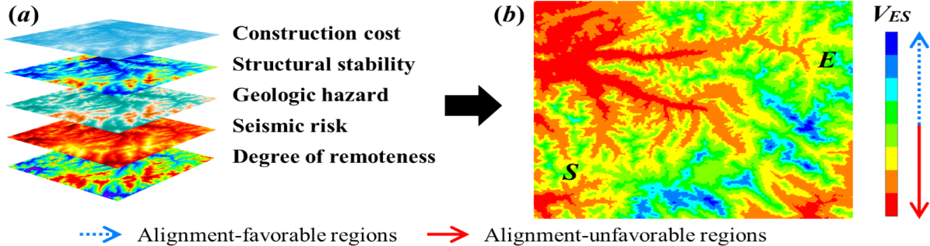
Figure 2.

(a) Environmental suitability influential factors and (b) environmental suitability map for alignments.

(1) An environmental suitability analysis and a DBSCAN clustering algorithm are performed on the study area before alignment search process for capturing the distribution characteristics of AFRs, as shown in Fig. 1. Subsequently, a specific criterion is developed to differentiate between IIEs and the other two AFRs distribution patterns, namely continuously-distributed AFRs and obstructed effects.
(2) The IIEs in the study area are abstracted as a semantic topological map (STM) for facilitating a subsequent path generation stage. Specifically, between-island paths are generated based on the relative locations of AFRs and through a designed multi-directional scanning process. Meanwhile within-island paths are determined using the endpoints of between-island paths and a conventional Floyd-Warshall algorithm. To this end, alignment optimization problem in the study area with densely-distributed obstacles is transformed into a shortest path problem on a graph. Consequently, this can efficiently generate optimized paths using conventional shortest path algorithms, such as Dijkstra’s, which is adopted in this paper.

The remainder of this work is organized as follows: Section 2 presents the land parcel preprocessing procedures. Section 3 introduces the construction process of the STM. Section 4 shows the alignment optimization method. Section 5 provides a realistic case study and Section 6 concludes this study.

2.Land parcel preprocessing

2.1Environmental suitability analysis for alignments

First, according to the resolution of the digital elevation model (DEM) used at the area-corridor railway design stage [36, 37], the study area is abstracted into a set of grid cells. Ground elevations, geo-hazard regions and unit structural costs are then stored in each grid cell, forming the essential railway design data. Subsequently, an environmental suitability analysis for alignments is conducted on this grid set [37]. In Pu et al. [37], multiple topographic and geologic factors are integrated to determine an environmental suitability value (V𝐸𝑆) for each grid cell. The evaluation of a grid cell’s environmental suitability accounts for the impacts of construction cost, stability, geologic hazard and seismic risk for different railway structures, as well as the degree of remoteness:

(1)

V𝐸𝑆=∑i=15(ωi⋅xi)

where xi is the nondimensionalized value (i.e., ranging from 0 to 1) for the construction cost, stability, geologic hazard, seismic risk or degree of remoteness for the grid cell and ωi is the criterion weight for the ith influencing factor. It is noteworthy that the relative significance of different indicators is determined using a multi-criteria decision-making method known as CRITIC (criteria importance through inter-criteria correlation). This method involves assigning weights to various indicators based on their values across the entire study area. Indicators exhibiting higher variance and lower correlation are assigned higher weights. Detailed formulations can be found in Pu et al. [37].

Figure 2 displays an environmental suitability map for alignments, where grid cells with higher V𝐸𝑆 values are considered preferable for traversing alignments. To distinguish between alignment-favorable and unfavorable regions, an environmental suitability threshold for alignments (T𝐸𝑆) is assigned. Grid cells with V𝐸𝑆 values exceeding the T𝐸𝑆 are classified as alignment-favorable grid cells (AFGs), while the remaining grid cells constitute alignment-unfavorable grid cells (AUGs). The threshold value assigned to AFGs and AUGs plays a critical role in establishing the distribution pattern of AFGs. In this paper, the threshold is determined based on the environmental suitability value corresponding to the inflection point (Pi⁢n) of the cumulative probability distribution curve (F⁢(x)). The curve F⁢(x) is constructed by fitting the cumulative frequency of each distinct V𝐸𝑆 value in ascending order. The frequency (F⁢(xi)) of the ith V𝐸𝑆 value is formulated according to Eq. (2).

(2)

F⁢(xi)=∑j=1iF𝐸𝑆𝑗N

where F𝐸𝑆𝑗= the number of jth environmental suitability value (j⩽i); N= the total number of grid cells in the entire study area.

From a statistical standpoint, P𝑖𝑛 signifies a discontinuous change in F⁢(x), depicted as a distinct bend or steep turn in the curve as illustrated in Fig. 3. Notably, at P𝑖𝑛, there is a marked alteration in the distribution of V𝐸𝑆 values, indicating a clear boundary between two sides of V𝐸𝑆 values. Hence, the V𝐸𝑆 value corresponding to P𝑖𝑛 is designated as the T𝐸𝑆, demarcating between AFGs and AUGs. The precise position of P𝑖𝑛 is determined where the second-order derivative of F⁢(x) equals 0, as specified in Eq. (3).

(3)

f⁢(T𝐸𝑆)=d2⁢F⁢(x)d⁢x2=0

Figure 3.

Demonstration of the cumulative probability distribution curve of environmental suitability values.

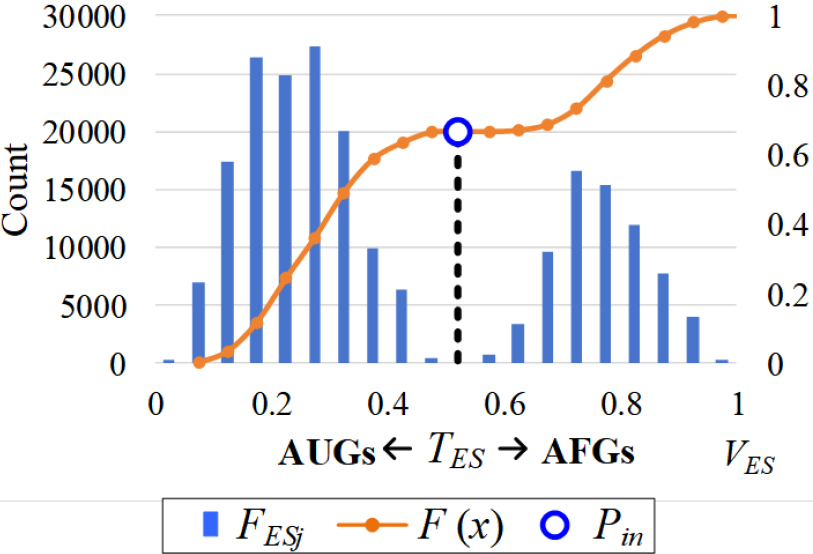
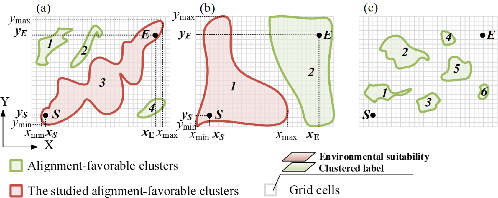
Figure 4.

Alignment-favorable clusters are (a) continuous; (b) obstructed and (c) isolated.

2.2Land parcel distribution pattern recognition

After deriving the alignment environmental suitability values of each grid cell, AFGs must be clustered into a set of AFRs with various shapes and scales for the subsequent construction of a STM. Spatial clustering approaches play a crucial role in identifying different AFR patches by grouping similar grid cells based on both their environmental suitability values and spatial relative locations into clusters.

However, AFRs often have irregular shapes, presenting challenges in accurately locating and determining their scales. Traditional clustering algorithms, such as the commonly used k-mean clustering algorithm [38], may require a predetermined cluster number and prove ineffective for clustering irregularly shaped groups. To address this challenge, a density-based clustering algorithm known as DBSCAN (Density-Based Spatial Clustering of Applications with Noise) is employed. DBSCAN can identify clusters of arbitrary shapes without requiring prior knowledge of the number and centers of clusters [39, 40]. In the DBSCAN algorithm, a point is classified as a core point if the number of neighboring points, called seed points, within a specified radius (ε) exceeds a certain threshold. This algorithm requires two key parameters: the radius (ε) and the minimum number of points (Nmin). A customized flow of the DBSCAN algorithm for identifying the distribution pattern of AFRs is presented below:

Step 1: Initialize all grid cells as unclassified and set T= 1.
Step 2: Starting from the top left and moving towards the bottom right, examine each unclassified grid cell to determine if it qualifies as a core point using the parameters ε and Nmin. A grid cell is designated as a core point (GP) and assigned to cluster CT if the number of alignment-favorable grid cells within a circle centered at the grid cell with a radius ε exceeds the predefined threshold N𝑚𝑖𝑛. Its seed points (GS) are recorded accordingly in a set called Ω. Otherwise, proceed to the next grid cell.
Step 3: Select GS from Ω, add it to cluster CT, mark it as classified, and remove it from Ω.
Step 4: Check if GS qualifies as a core point with the parameters ε and Nm⁢i⁢n. If it does, add its unclassified seed points to Ω. If it does not, return to Step 3.
Step 5: Repeat Steps 3 and 4 until all grid cells in Ω are classified.
Step 6: Increase the value of T by 1 (T=T + 1), and repeat Steps 2 to 5 until no more core points remain.
Step 7: Assign grid cells that do not belong to any cluster as noise.

After implementing the DBSCAN algorithm, the AFRs are grouped into clusters, and each grid cell is assigned a cluster label (CT) accordingly. Subsequently, the distribution pattern of AFRs is determined by the relative locations of the clusters with respect to the start and end points. The specific identification formulas are:

(4)

xmin⩽min⁡(xS,xE);xmax⩾max⁡(xS,xE)

(5)

ymin⩽min⁡(yS,yE);ymax⩾max⁡(yS,yE)

where xmin, ymin, xmax, ymax= the minimum and maximum boundaries of each alignment-favorable cluster and xS, yS, xE, yE= the coordinates of the start and end points.

If a cluster of AFRs satisfies the criteria stated in both Constraints (2) and (3), the AFRs are continuous throughout the study area (Fig. 3a). However, if none of the alignment-favorable clusters satisfy Constraint (2) but at least one cluster satisfies Constraint (3), the AFRs are concentrated within the study area (Fig. 4b). Otherwise, AFRs’ distribution pattern presents an IIEs, as shown in Fig. 4c.

The purpose of clustering AFRs is to efficiently generate paths within and between AFRs using specific strategies in the following path development process. However, the shape of AFRs is extremely irregular, and can be generally divided into convex and concave polygons. The complex shape of the convex polygons is very detrimental to efficient connection between them. Therefore, to facilitate subsequent separated path generation procedures, AFRs are unified as convex polygons by identifying and transforming concave polygons into convex polygons [41]. The specific steps are listed as follows:

Step 1. Connect the vertexes (A, A1, …, An) of an AFR in a clockwise direction. Then, identify whether the shape of this AFR is a concave polygon with the following formulas:

(6)
{A0⁢A1¯×A1⁢A2¯<0A1⁢A2¯×A2⁢A3¯<0⋯An-2⁢An-1¯×An-1⁢An¯<0

where An-2⁢An-1¯×An-1⁢An¯= the vector cross product of the vector at An-2 and An-1 with the vector at An-1 and An. If the value of this vector cross product exceeds 0, this polygon is concave at An-1, as shown in Fig. 5b. Otherwise, this AFR presents a convex shape as shown in Fig. 5a.
Step 2. Extend An-2⁢An-1¯ in the direction of this vector to split this polygon into two sub-polygons (i.e., PP⁢1 and PP⁢2 in Fig. 5c).
Step 3. Repeat Steps 1 and 2 to check whether these are convex polygons, until all the sub-polygons are convex.

3.Isolated island effect representation

3.1Structure of semantic topological map

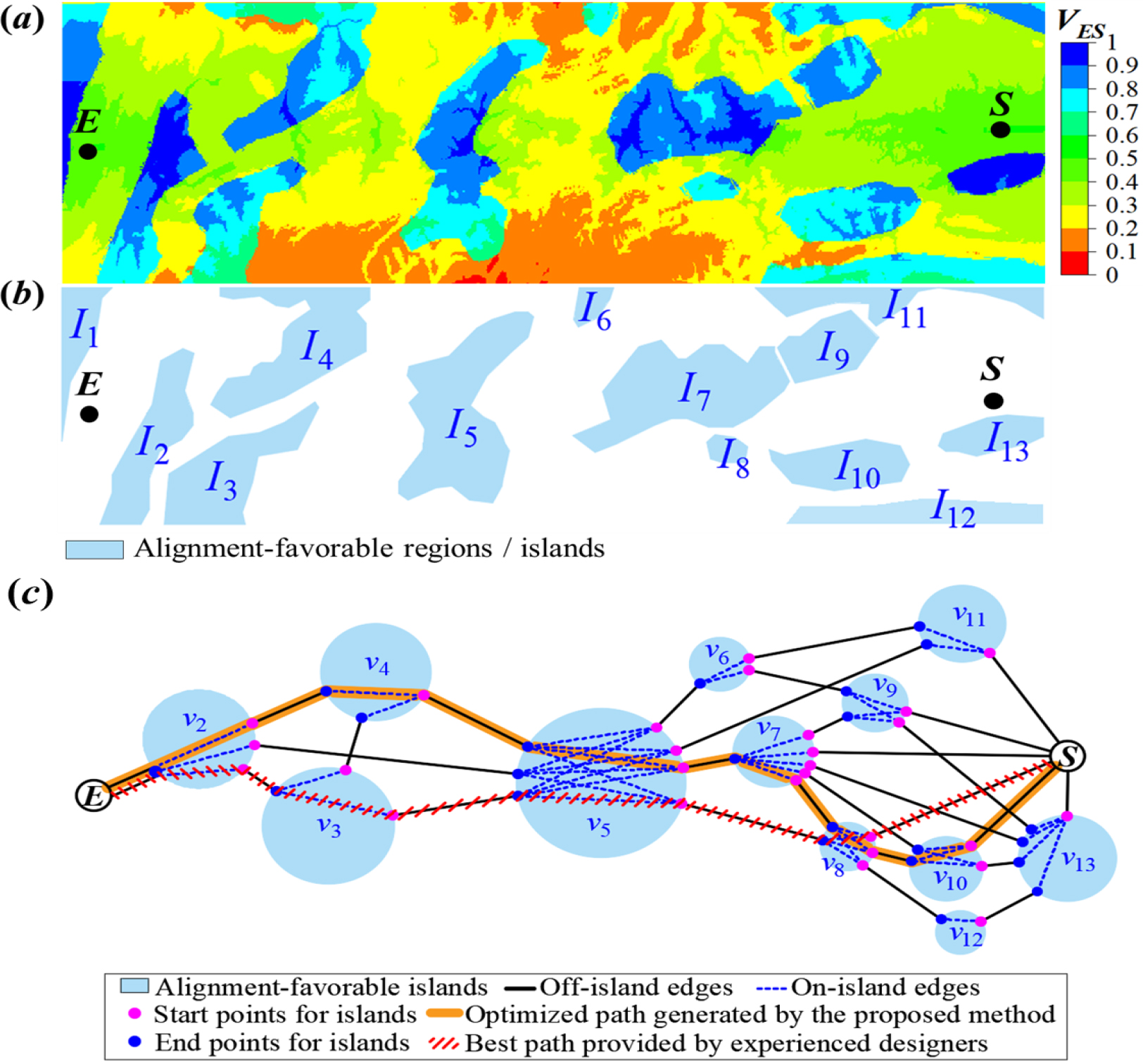
In this study, the focus is on alignment development in a study area exhibiting an IIE, where each alignment-favorable cluster is called an island. To effectively utilize the island distribution features and assist the alignment optimization process, a specific data structure is required to represent these features. A semantic topological map (STM), which comprises nodes and edges, can provide an intuitive and easily understandable visualization of the complex system under investigation [42]. Therefore, the island distribution features are abstracted and represented as an STM, denoted as G. The topology structure of this STM can be expressed as:

(7)

G=(V,PS,PE,Eo⁢f⁢f,Eo⁢n,WE⁢o⁢f⁢f,WE⁢o⁢n)

where V= {v1, v2, …, vn} denotes a set of temporary nodes that store the locations and scales of islands, n= the number of islands; PS= {ps⁢1, ps⁢2, …, p𝑠𝑛} and PE= {pe⁢1, pe⁢2, …, p𝑒𝑛} represent the start and end nodes set for every island; E𝑜𝑓𝑓= {e12, e13, …, ei⁢j} indicates a set of off-island edges, where ei⁢j⁢(vi,vj) is the off-island edge connecting vi and vj (among which, vi and vj represent two temporary nodes directly connected, vi is a former node and vj is a latter node); E𝑜𝑛= {eo⁢n⁢1, eo⁢n⁢2, …, e𝑜𝑛𝑖} denotes on-island edges, where e𝑜𝑛𝑖(p𝑠𝑖, p𝑒𝑖)= the on-island edges connecting each pair of start and end points of vi; W𝐸𝑜𝑓𝑓,W𝐸𝑜𝑛= the alignment suitability costs set for the off-island edges and on-island edges, respectively.

For the STM, a graph adjacent matrix (AM) is used for describing the adjacency relations between every island pair:

AM={ai⁢j}n×n

(8)

ai⁢j={1, if ⁢ei⁢j⁢(vi,vj)∈Eo⁢f⁢f0, if ⁢ei⁢j⁢(vi,vj)∉Eo⁢f⁢f

where ai⁢j is the element in the ith row and jth column for AM, while n is the number of islands. It is noted that ai⁢j= 1 means vi and vj are adjacent in an STM.

In the STM representing the island distribution features, it is important to consider that an island may have multiple start and end nodes. To capture the connectivity information among these nodes, the connecting conditions of each start and end node pair are stored in on-island edges specific to that particular island. Each edge represents the connection between a start node and an end node, and there can be multiple such connections within the island. Therefore, to fully represent the connectivity within the island, p×q on-island edges are required for an island with p start nodes and q end nodes.

3.2Constructing a semantic topological map

The construction of a STM involves two key procedures: between-island connectivity and within-island path determination.

3.2.1Between-island connectivity

In this procedure, alignment-favorable clusters are treated as temporary nodes, and their adjacency relations are recorded in off-island edges. The temporary nodes are assigned numbers based on the coordinates of their centers of gravity. To assign these numbers, the centers of gravity of all nodes are projected onto an x-axis, and the nodes are numbered sequentially from left to right, starting from 1. If there are multiple nodes with the same x-coordinate, their numbers increase as the y-coordinate increases. After the temporary nodes are numbered (as shown in Fig. 6a), the locations of the off-island edges and their alignment suitability costs are determined using a devised multi-directional scanning process. This scanning process involves systematically scanning the study area with line segments in different directions, as shown in Fig. 7. These scanning line segments, denoted as L, can be expressed as follows:

𝑳=Y2∪Y3

(9)

{Y1=YE-YSXE-XS⋅X+XE⋅YS-XS⋅YEXE-XSY2=Y1+N⋅WY3=R⁢(Y2)

X∈[XL,XR];

N∈[-YU-YD2⋅W,⋯,0,1,⋯⁢YU-YD2⋅W]

where Y1= the base scanning line crossing the start and end points; Y=2 the translational scanning line set derived by translating Y1 upwards and downwards at the spacing of the grid cell width; Y=3 the rotational scanning line set obtained by rotating Y 2n times (i.e., 36) with rotation angles 5^∘, 10^∘, …, 180^∘; X, Y= the design variables of L, representing the coordinates of the points located on the scanning lines; XL, XR= the left and right boundaries of X; YU, YD= the upper and lower boundaries of Y; N= the number of translational lines; W= the width of a grid cell and R= the rotation transformation of a line, whose rotation angle (α) ranges from 0^∘ to 180^∘ at 5^∘ intervals in this study.

Figure 5.

AFRs in the shape of (a) a convex polygon; (b) concave polygon and (c) division of concave polygon into convex polygons.

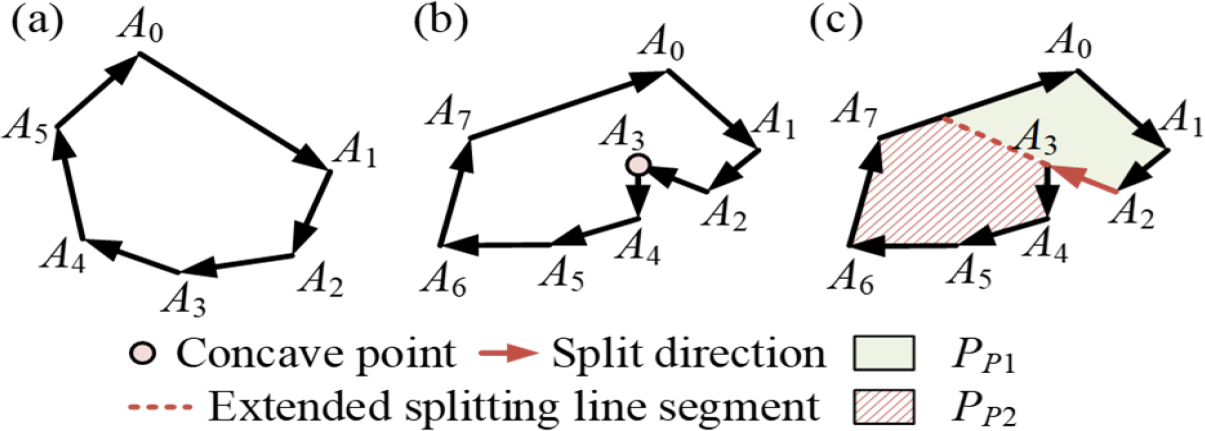
Figure 6.

(a) The AFRs distribution in a study area with an IIE; (b) temporary nodes decomposition and (c) the finial topology structure of the STM.

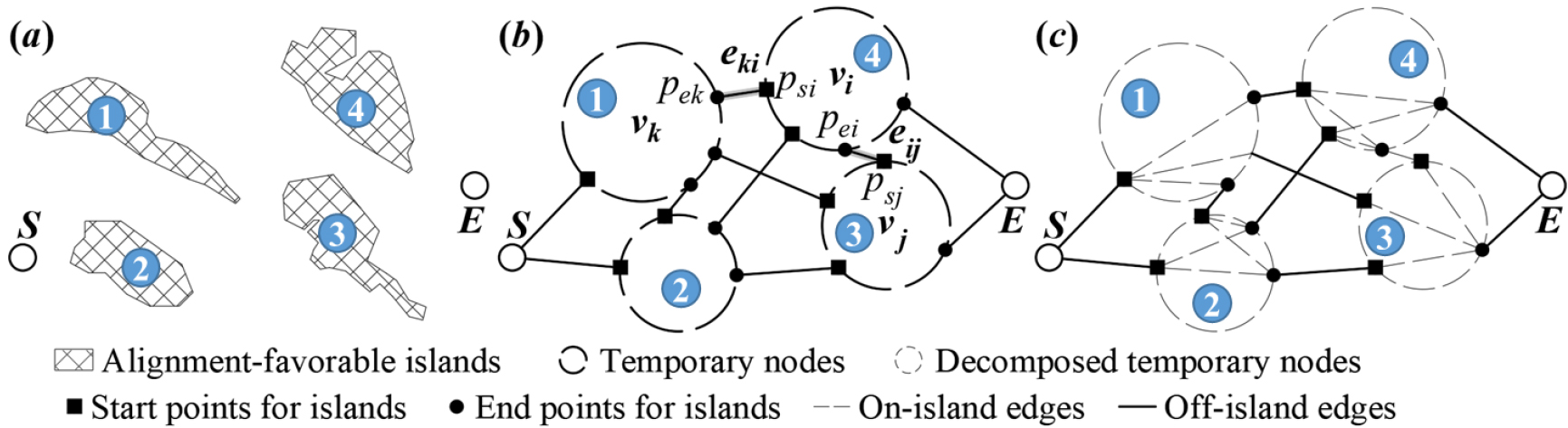
Figure 7.

Scanning lines and the line segments between two alignment-favorable regions (i.e., temporary nodes).

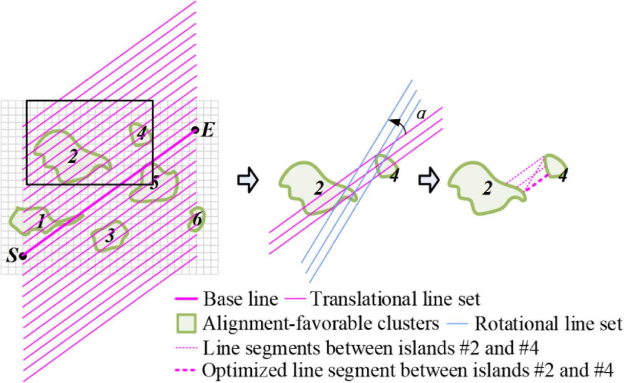
By implementing this multi-directional scanning strategy, the optimized connection between any two AFRs islands can be derived with the following procedures:

Step 1. Determine the former and latter nodes:
Intercept the line segments connecting islands vi and vj from the previously mentioned set of multi-directional scanning lines (L). Define the endpoints of these line segments located on island vi (or vj) as Pe⁢i (or Ps⁢j).
Compute the distances of Pe⁢i and Ps⁢j from the start point.
If Pe⁢i is closer to the start point, it is designated as the former node.
Pe⁢j is defined as the latter node.
Step 2. Record the directed line segments:
The directed line segments connecting vi and vj is recorded in the line segments set Φi⁢j
Step 3. Compute the environmental suitability cost (CL) of line segments in Φi⁢j. Specifically, CL is computed by accumulating the difference between the maximum V𝐸𝑆 (V𝐸𝑆𝑚𝑎𝑥) in the study area and the V𝐸𝑆 value of every grid cell traversed by this line segment. Assuming that the line segment traverses N grid cells the environmental suitability cost, CL is computed as:

(10)
CL=∑k=1N(V𝐸𝑆⁢max-V𝐸𝑆𝑘)

Afterward, the line segment with the minimum CL value is designated as the edge (ei⁢j) between vi and vj. Then, ai⁢j of ei⁢j is assigned as 1, and W𝐸𝑜𝑓𝑓 for ei⁢j is:

(11)

W𝐸𝑜𝑓𝑓⁢(ei⁢j)=min⁡CL⁢(xi,yi,xj,yj)

where xi, yi⁢xj, yj, are the coordinates of two endpoints (pe⁢i, ps⁢j) of the line segment with the minimum environmental suitability cost. These endpoints are stored in the variable ei⁢j, which provides the start and end points for generating subsequent paths within each temporary node. It is important to note that for an edge ei⁢j, pe⁢i represents an endpoint of vi, while ps⁢j represents a start point of vj, as shown in Fig. 6b.

3.2.2Within-island path determination

To generate paths within a temporary node (vi) that has multiple start and end points, the node is further decomposed based on these points. Each start and end point is treated as a separate node, and all pairs of start and end points are connected to determine the on-island edges. The weight of each on-island edge (W𝑜𝑛𝑖) is assigned as the minimum accumulating environmental suitability cost of the paths between the corresponding endpoints. Handling multiple start and end points within a temporary node can be viewed as a Multi-Source Shortest-Path (MSSP) problem. The Floyd-Warshall algorithm [43] is a typical MSSP algorithm that can find the shortest paths between all pairs of nodes in a graph. It is both intuitive and easy to implement. Thus, it is used in this work for efficiently determining the optimized paths. To apply the Floyd-Warshall algorithm to the optimization of on-island paths, two adaptations are made, addressing the study area and the traditional Floyd-Warshall algorithm separately.

1. Regarding the study area, a sub-graph representing the study area within each temporary node is constructed. Using a circular-shaped window mask, as proposed by Song et al. [3], every grid cell within the temporary node is scanned. Grid cells satisfying the design constraints, including the center grid cell and its boundary grid cells, are designated as nodes in the sub-graph. The lines connecting the center grid cell with the boundary grid cells are considered as edges in the sub-graph.
2. Simultaneously, the Floyd-Warshall algorithm is parallelized for the optimization of on-island paths within each node. In more detail, during the between-island paths determination procedure, the start and end points of each node are obtained and designated as the input for the Floyd-Warshall algorithm. Consequently, all optimized within-island paths can be derived through a single loop of the Floyd-Warshall algorithm, eliminating the need to sequentially traverse every node.

Figure 8.

Path generation process of Dijkstra’s algorithm.

Afterward, the Floyd-Warshall algorithm is applied to each sub-graph until the costs from the start points to the end points are stabilized, ensuring the optimized paths are determined.

By following these procedures, an STM is generated (as shown in Fig. 6c), representing the distribution characteristics of islands. Additionally, environmental suitability costs are assigned to each node and edge within the map, providing valuable information for further alignment search processes.

4.Alignment optimization method

4.1Alignment search process

In the alignment optimization process, the STM with determined edge suitability is used. Dijkstra’s algorithm, known for its effectiveness in path optimization problems, has been successfully applied in various contexts, including alignment optimization [3, 44]. It is also employed in this paper. Dijkstra’s algorithm, as applied to alignment optimization, is outlined below:

Step 1: Add all the nodes in the STM to a node set, NS.
Step 2: Designate two arrays for each node: one for storing the environmental suitability cost (dis[v]), and another for storing its former adjacent node in the optimized path from the start point (for[v]). Initialize dis[v] as infinity for all nodes, except for the start point which is assigned a value of 0. The former adjacent node for the start point is itself, while the values in for[v] for other nodes are undefined.
Step 3: Choose the node, vi, with the minimum dis[vi] value from NS and remove it from NS. Find all the latter adjacent nodes (VL) of vi from NS. Latter adjacent nodes refer to nodes that are farther from the start point than vi, as stated in Section 3.2 of the paper.
Step 4: Compute the environmental suitability cost (WE⁢(ei⁢j)) from a latter adjacent node (vj) to vi. If dis[vi] +WE⁢(ei⁢j) is less than the current dis[vj] value, update dis[vj] as dis[vi] +WE⁢(ei⁢j) and set for[vj] as vi
Step 5: Repeat Step 4 until the dis[v] and for[v] values of all the latter adjacent nodes have been updated.
Step 6: Repeat Steps 3 to 5 until there are no elements left in NS.

By following these steps, Dijkstra’s algorithm computes the distance (environmental suitability cost) from each node to the start point, while also storing the predecessor (former adjacent node) in the optimized path. This process continues until all nodes have been visited and processed, resulting in an optimized alignment that considers environmental suitability costs between nodes. Specifically, an optimized path development process between an observed node and the start point is shown in Fig. 8.

4.2Constraints

In the process of generating a railway alignment, it is necessary to consider multiple constraints related to geometric, structural, and locational aspects. These constraints ensure that the alignment satisfies the necessary design criteria and construction limitations, while avoiding sensitive or forbidden regions.

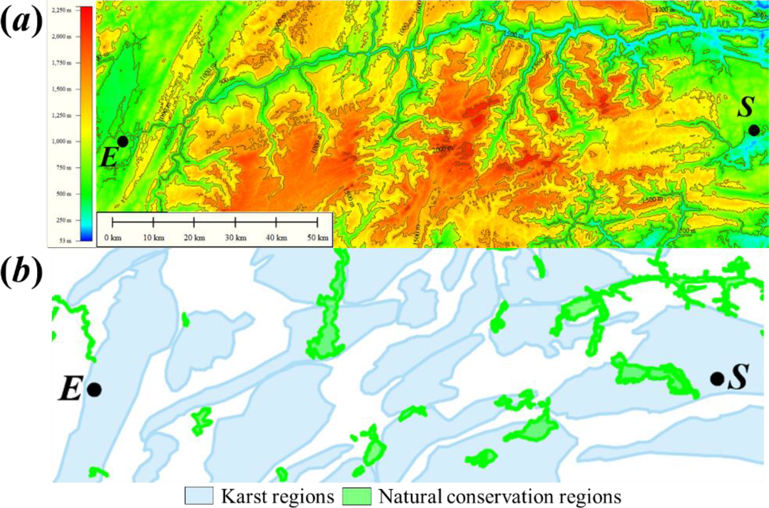
Figure 9.

(a) The terrain and (b) the geology maps of the study area.

(1) The geometric constraints focus on ensuring that the alignment profile adheres to the specific design criteria for railways. These criteria may include considerations such as vertical and horizontal clearances, minimum curve radius (Rm⁢i⁢n), and maximum gradient.
(2) Structural constraints take into account the limitations of the available construction techniques. They consider factors such as the type of terrain, soil conditions, and construction equipment capability. These constraints ensure that the alignment can be constructed safely and efficiently.
(3) Locational constraints primarily revolve around avoiding environmentally sensitive areas and forbidden regions. This includes areas with protected flora and fauna, cultural heritage sites, residential areas, and other designated areas that should be avoided due to legal or social reasons.

As outlined in Section 1, the primary contribution of the proposed method lies in generating an optimized alignment corridor during the area-corridor stage, intended to provide an initial alternative for the subsequent corridor-alignment optimization stage.

The corridor-alignment optimization typically involves two steps:

Step 1: The initial output, representing the optimized path solution from the proposed method, is subjected to a fitting process. This process involves configuring curves with a minimum allowable radius (Rmin) to points of intersection (PIs) along the optimized path. Detailed procedures, as described in Li et al. [45], are followed to check the corresponding minimum allowable tangent lengths.
Step 2: To ensure alignment re-optimization after deviations from the initial optimized path, nature-inspired optimization methods such as genetic algorithms (GA) and particle swarm optimization (PSO) are employed. These methods iteratively adjust the locations of PIs within a specific corridor, defined by the optimized path as the centerline and a designated width as a buffer zone. The adjustment process continues until the objective function of the alignment optimization converges to an optimized value.

It is noted that the generated alignment alternatives must adhere to the aforementioned alignment design constraints.

Table 1

Unit costs

Item	Value	Item	Value
Rail track (10⁴¥/m)	0.46	Right-of-way (¥/m²)	13.4
Fill earthwork (¥/m³)	65	Cut earthwork (¥/m³)	32
(100 m < h < 150 m) Bridge (10⁴ ¥/m)	15	(h < 100 m) Bridge (10⁴¥/m)	14
(L < 1 km) Tunnel (10⁴¥/m)	11.5	(1 km < L < 4 km) Tunnel (10⁴¥/m)	10.5
(L > 4 km) Tunnel (10⁴¥/m)	13.5	One bridge abutment/tunnel portal (10⁴¥)	20

5.Case study

5.1Case profile

In this study, the focus is on the W-E High-Speed Railway (HSR), which is a railway under construction. The railway has a maximum design speed of 350 km/h and spans a distance of 153 km. It is located in the southwest region of Hubei Province, where there is a significant presence of karst landforms in the undulating mountainous areas [46]. Karst landforms are formed due to the long-term effects of groundwater and surface water on soluble rocks, resulting in unique features such as gullies, funnels, and caves. These landforms pose potential risks to railway alignments, particularly in tunnel sections [47, 48]. Karst geological disasters like collapses, water invasion, and mud gushing can severely impact tunnel construction, causing damage to equipment and even casualties [49, 50]. The YiChang-Wanzhou railway, which is a section of the HSR in this study area, has already been constructed and faced significant challenges in dealing with karst hazards along its route [49]. Therefore, it is desirable to completely bypass karst landforms when planning the alignment for the W-E HSR. However, when the railway is situated in a mountainous region with undulating terrain and dense karst landforms, it becomes highly likely that the alignment will encounter karst areas. In such situations, it is important to ensure that there is sufficient clearance between the alignment and karst regions, satisfying the required safety standards, considering topologic and geologic conditions. Moreover, the study area also includes multiple natural conservation areas, which must be traversed using bridges or tunnels in order to minimize environmental impact. In total, there are 19 karst regions and 14 natural conservation areas within the study area, covering a significant fraction of the terrain. Terrain and geology maps for the study area, as well as unit costs for railway construction, are obtained from the China Railway Siyuan Survey and Design Group Co. Ltd., as demonstrated in Fig. 9 and Table 1, respectively.

It is notable that the terrain in this area is characterized by significant undulations, with a maximum elevation difference of 2,197m. Therefore, the maximum allowable gradient (Gmax) for the railway is set at 30‰ taking into account the steepness of slopes. Considering the topography in optimizing the design, it is advisable to create vertical alignments that follow the natural undulations of the terrain. This approach helps to reduce tunnel lengths and control bridge heights, thus minimizing construction costs and potential environmental impacts. The karst landforms are densely distributed throughout the entire study area, leaving only narrow and irregular non-karst areas. Thus, the railway alignment is highly likely to encounter karst regions along its route. Given the potential risks associated with karst hazards, it is essential to plan the alignment carefully in order to avoid or mitigate these challenges. Bypassing karst areas entirely and ensuring a sufficient clearance between the alignment and the karst regions should be a priority for ensuring the safety and stability of the railway construction.

Figure 10.

(a) Environmental suitability map for alignments; (b) the distribution of AFRs; (c) semantic topological map of the study area.

5.2Results

5.2.1Land parcel treatment

(1) Environmental suitability distribution

The environmental suitability map of the study area is generated using Eq. (1) and presented in Fig. 10a. Subsequently, the cumulative probability distribution curve, as illustrated in Fig. 11, is obtained for all environmental suitability (V𝐸𝑆) values by applying the second derivative to Eq. (2). The threshold V𝐸𝑆 value (T𝐸𝑆) demarcating AFRs and AURs is then computed using Eq. (3), and in this case, the threshold value is set at 0.5.

In this regard, the grid cells with a V𝐸𝑆 value exceeding T𝐸𝑆 are identified as AFRs for the railway. It is observed that approximately 33.4% of the study area consists of AFRs, but most of them are isolated and surrounded by AURs.

(2) Alignment-favorable regions clustering

The radius (ε) and the minimum number of points (Nmin) are two crucial parameters in the DBSCAN algorithm, significantly influencing the scales and number of clusters. In this scenario, opting for a smaller ε is preferred to prevent different obstacles from being clustered into the same group. Accordingly, ε is set as the minimum distance between two obstacles, and the value of Nmin is set to 90% of the result obtained by dividing the area of a circle with ε as the radius by the area of the grid cell. Once these key parameters are established, the DBSCAN clustering algorithm is applied to identify distinct AFRs. This algorithm accurately pinpoints the locations and scales of these regions, referred to as islands in this study. In the present case, 13 islands are identified, as depicted in Fig. 10b.

(3) Construction of semantic topological map

Through the specific multi-directional scanning process and the implementation of the Floyd-Warshall algorithm, a STM is constructed, including the sequential generation of between-island and within-island paths, as shown in Fig. 10c.

5.2.2Alignment solutions

Following the construction of the STM, an alignment optimization process is carried out based on this map. It turns out that the path optimized in this process traverses islands 10, 8, 7, 5, 4, and 2, as determined by the proposed method. In comparison, the alignment provided by human designers traverses islands 8, 5, 3, and 2. It is noteworthy that the proposed method selects additional islands (10, 7, and 4) that were not considered in the human-designed alignment. This result highlights that the constructed STM offers diverse alignment alternatives for railway design. The proposed method provides an expanded range of options by considering additional islands, thereby allowing for a more comprehensive exploration of possible alignments.

Figure 11.

Cumulative probability distribution curve of V𝐸𝑆 values.

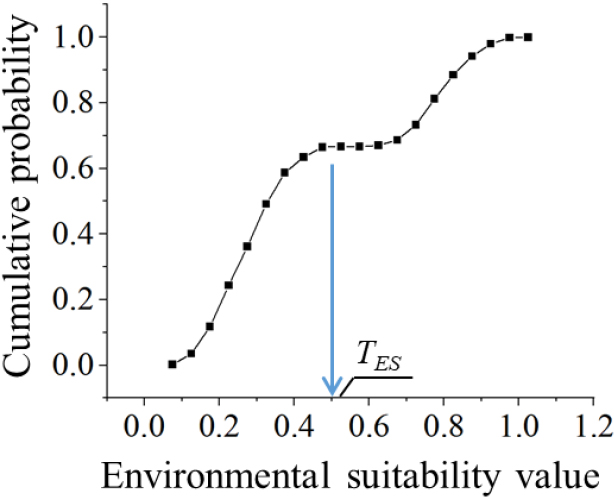
Figure 12.

Horizontal alignments of AM, AD and AS.

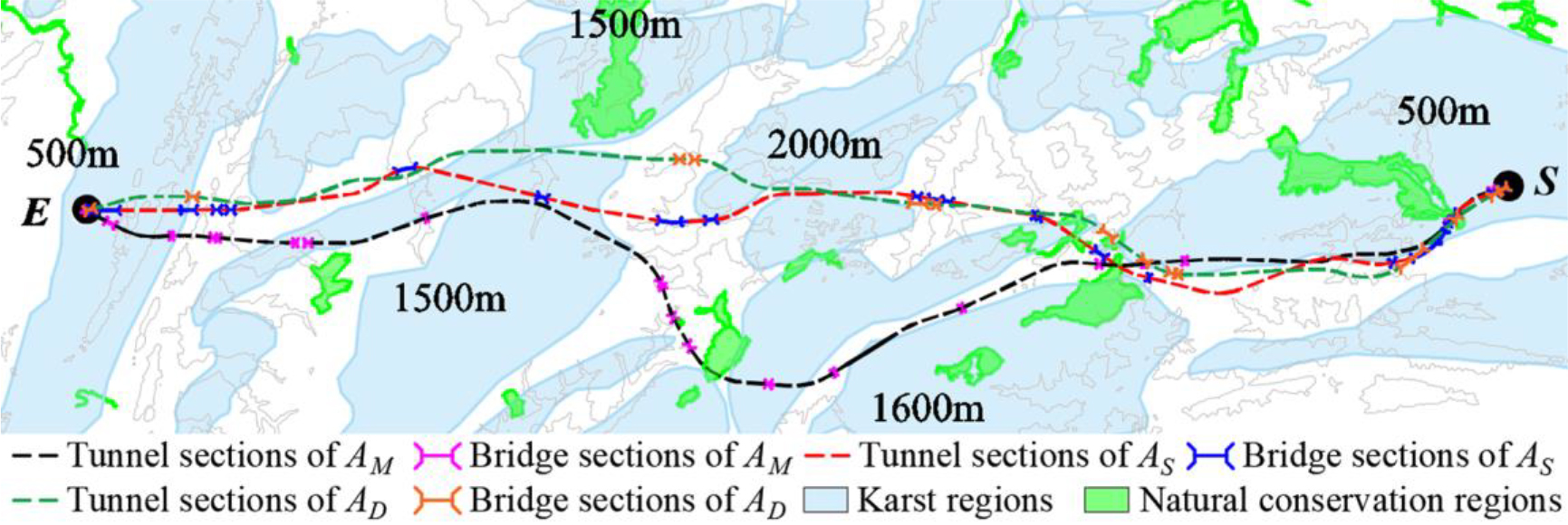
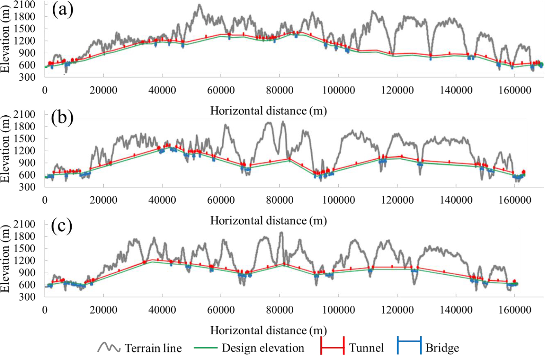
Figure 13.

Vertical alignments of (a) AM (b) AD and (c) AS.

Subsequently, the optimized path is fitted using the method described in Section 4.2, and the derived initial alignment alternative serves as input to a previously established PSO method [23] for generating the detailed alignment solution.

In this paper, a previous environmental suitability analysis-assisted 3D-DT (ES-3D-DT) algorithm from Pu et al. [34] is taken as a benchmark method to showcase the effectiveness of the proposed method in solving alignment optimization problems within study areas characterized by densely-distributed obstacles.

In the ES-3D-DT method, the study area is represented as a set of voxels, and the V𝐸𝑆 values for all feasible voxels is computed using Eq. (1). Subsequently, environmental suitability grades (Grade I, II, and III) are assigned based on the derived V𝐸𝑆. During the alignment search, voxels with Grade III environmental suitability, indicating unfavorable for alignments, are excluded from consideration. The detailed flow chart of the ES-3D-DT method can be found in Pu et al. [34].

Table 2

Numerical comparisons of AM, AD and AS

Item	A_M	A_D	A_S
Railway length (m)	168,739	163,311	160,974
Right-of-way area (m²)	357,903	347,691	352,962
Filling/Cutting volume (m³)	24,949/151,751	25,638/163,522	25,093/161,305
Number of bridges (100 m < h < 150 m)-Total length (m)	25–19,573	22-20,219	14–11,852
Number of bridges (h < 100 m)-Total length (m)	3–2,461	4–5,873	10–13,159
Total number-length of bridges (m)	28–22,034	26–26,092	24–25,011
Number of tunnels (L < 1 km)-Total length (m)	13–7,396	6–3,819	8–3,449
Number of tunnels (1 km < L < 4 km)-Total length (m)	15–35,265	10–19,930	4–8,481
Number of tunnels (L > 4 km)-Total length (m)	10–103,881	10–109,047	11–117,729
Total number-length of tunnels (m)	38–146,542	26–132,796	23–129,659
Total bridge length in karst regions (m)	8,909	6,530	10,685
Total tunnel length in karst regions (m)	75,628	54,960	42,899
Total alignment length in karst regions (m)	84,537	61,490	53,584
Total alignment length in natural conservation regions (m)	3,386	2,355	3,135
Total construction cost (million ¥)	22,530	21,780	21,618
Improvement	N/A	3.3%	4.0%
Alignment suitability cost	2,690	2,548	2,415
Improvement	N/A	5.3%	10.2%

Both the ES-3D-DT and the proposed method are executed on a computer with Intel Core i7-7700 CPU @ 3.60 GHz, with the grid resolution of the study area set at 30 m. The ES-3D-DT method requires 135 minutes to produce the optimized alignment corridor. In contrast, the proposed method leverages Dijkstra’s algorithm to generate the optimized path based on the derived STM within a significantly reduced time frame of 113 seconds. Considering that the time to construct the STM is 621 seconds for this case, the proposed method notably enhances the efficiency of the alignment corridor optimization process. Afterward, the best corridors derived from both ES-3D-DT and the proposed method are refined with the customized PSO for obtaining the detailed alignment solutions, designated as AD and AS, derived from the corridors created by ES-3D-DT and the proposed method, respectively. AD and AS are further compared with the best alignment (AM) provided by experienced designers from the China Railway Siyuan Survey and Design Group Co. Ltd. Their horizontal and vertical alignments are shown in Figs 12–13, and detailed comparison data are provided in Table 2.

Based on the observations and comparisons, several key findings can be highlighted:

(1) Both AD and AS result in shorter railways (i.e., 5,428m and 7,765m for AD and AS, respectively) compared to AM. These reductions contribute to a smoother geometric profile of the HSR, which is advantageous for subsequent railway operation and maintenance stages.
(2) In comparison with AM, the total tunnel lengths decreased significantly by 13,746m and 16,883m, while the total bridge lengths increased slightly by 4,058m and 2,977m for AD and AS, respectively. By shortening the expensive tunnels, the construction costs for AD and AS are reduced by 3.3% and 4.0%, respectively.
(3) In terms of the karst hazard avoidance, AD decreases the length of alignment sections that traverse karst hazard regions, including shortening most karst-sensitive tunnels compared to AM. AS performs even better than AD by further reducing alignment and tunnel lengths in karst regions.
(4) Concerning natural conservation regions, AD exhibits the best performance by reducing the length of alignment traversing sections to 2,355m compared to AM’s 3,386m. It can be found that AD effectively bypasses sparsely-distributed natural conservation regions, but struggles with densely-distributed karst regions compared to AS. Therefore, AS achieves the best performance, improving alignment environmental suitability cost by 10.2% compared to AM.

In summary, the analyses demonstrate that the proposed model and method (AS) outperform both the optimized alignment (AD) generated by the ES-3D-DT and the manually-designed alignment (AM) in terms of reduced karst coverage, lower construction cost, and improved environmental suitability. AS effectively optimizes the alignment by minimizing tunnel lengths and overall railway footprint. These findings highlight the potential value of using the proposed model and method to generate alignment alternatives that offer both cost efficiency and environmental benefits.

6.Conclusion

In the context of highly-constrained study areas, where alignment-favorable regions (AFRs) are isolated and alignment design is a challenging task, a novel approach is proposed here for addressing this problem. In this approach, environmental suitability analysis is employed to identify AFRs, while an STM is used to depict the distribution pattern of these AFRs. Through this process, the complicated alignment optimization problem is simplified into a shortest path problem, which can be effectively solved using conventional shortest path algorithms. The application of the proposed method in a realistic railway case has demonstrated several key findings:

(1) The method significantly enhances the efficiency of generating optimized alignment corridors within a densely-distributed karst alignment search space. Despite requiring several minutes (i.e., 621s) for land parcel treatment, the subsequent search process only takes 113 seconds, marking a substantial improvement compared to the 135 minutes needed for the ES-3D-DT method.
(2) Comparisons of alignment solutions highlight the effectiveness of the ES-3D-DT-generated alignment (AD) in outperforming the best manually designed alignment (AM). AD notably reduces construction and environmental suitability costs by 3.3% and 5.3%, respectively, underscoring the significance of environmental suitability analysis in ensuring the quality of alignments derived from computer-aided optimization methods. Moreover, the best alignment (AS) generated by the proposed method surpasses AD’s performance. AS achieves a reduction of 4.0% in construction costs and an improvement of 10.2% in environmental suitability costs compared to AM.

It is noted that the paper specifically focuses on a study area featuring multiple karst regions as an illustrative example. However, the proposed method is adaptable and applicable to all alignment search spaces characterized by IIEs.

Above all, the proposed method is effective in alignment optimization in a study area with densely-distributed obstacles in terms of computational efficiency and solution quality.

The limitations of this work include the following:

(1) In this paper, the threshold value of AFRs and RURs is set to the environmental suitability value corresponding to the inflection point of the cumulative probability distribution curve (which is a representation of distribution features of all the environmental suitability values across the study area). However, it becomes necessary to dynamically adjust this threshold value to ensure the aggregation of AFR patches, thereby expanding the applicability of the proposed method across a wider range of study areas. This issue warrants dedicated and specific studies, which the authors intend to undertake in their future research endeavors.
(2) Some existing methods are adopted in this work, such as the DBSCAN clustering algorithm as well as the Floyd-Warshall Dijkstra’s and PSO algorithms. It is important to highlight that these methods form part of a novel alignment optimization framework introduced in this paper. This framework involves three sequential steps: land parcel preprocessing, STM construction, and optimized path generation based on the derived STM. While these methods are integral to this framework, alternative approaches can be substituted that achieve similar functionalities. For example, other nature-inspired optimization methods such as a neural dynamic model [51], a harmony search algorithm [52], a simulated annealing [53] and a spider monkey optimization method [54] can also be explored for further confirming the effectiveness of the proposed optimization framework.
(3) Besides, other factors that affect railway alignment design, such as ecologic impacts and social influence, should also be specially-studied and integrated into the alignment traversing suitability analyses.

Acknowledgments

This work is partially funded by the National Key R&D Program of China with award number 2021 YFB2600403; National Science Foundation of China: 52078497; Science and Technology Research and Development Program Project of China railway group limited (2022-Major-20); the Fundamental Research Funds for the Central Universities of Central South University (2023ZZTS0378).

References

[1]	Vázquez-Méndez ME, Casal G, Castro A, Santamarina D. An algorithm for random generation of admissible horizontal alignments for optimum layout design. Computer-Aided Civil and Infrastructure Engineering. (2021) ; 36: (8): 1056-72. doi: 10.1111/mice.12682.
[2]	Shi J, Zhang Y, Chen Y, Wang Y. A smoothness optimization method for horizontal alignment considering ballasted track maintenance. Computer-Aided Civil and Infrastructure Engineering. (2023) ; 38: (6): 739-61. doi: 10.1111/mice.12884.
[3]	Song T, Pu H, Schonfeld P, Liang Z, Zhang M, Hu J, et al. Mountain railway alignment optimization integrating layouts of large-scale auxiliary construction projects. Computer-Aided Civil and Infrastructure Engineering. (2023) ; 38: (4): 433-53. doi: 10.1111/mice.12839.
[4]	Song T, Pu H, Schonfeld P, Zhang H, Li W, Hu J. Simultaneous optimization of 3D alignments and station locations for dedicated high-speed railways. Computer-Aided Civil and Infrastructure Engineering. (2021) ; 37: (4): 405-26. doi: 10.1111/mice.12739.
[5]	Hirpa D, Hare W, Yves Lucet, Yasha Pushak, Tesfamariam S. A bi-objective optimization framework for three-dimensional road alignment design. Transportation Research Part C-Emerging Technologies. (2016) ; 65: : 61-78. doi: 10.1016/j.trc..
[6]	Zhang H, Song T, Schonfeld P, Pu H, Li W, Hu J, et al. Vertical alignment optimization of mountain railways with terrain-driven greedy algorithm improved by Monte Carlo tree search. Computer-Aided Civil and Infrastructure Engineering. (2023) ; 38: (7): 873-91. doi: 10.1111/mice.12923.
[7]	Song T, Pu H, Schonfeld P, Zhang H, Li W, Hu J, et al. Mountain railway alignment optimization considering geological impacts: A cost-hazard bi-objective model. Computer-Aided Civil and Infrastructure Engineering. (2020) ; 35: (12): 1365-86. doi: 10.1111/mice.12571.
[8]	Karlson M, Karlsson CSJ, Mörtberg U, Olofsson B, Balfors B. Design and evaluation of railway corridors based on spatial ecological and geological criteria. Transportation Research Part D: Transport and Environment. (2016) ; 46: : 207-28. doi: 10.1016/j.trd.2016.03.012.
[9]	Zhu Z, Xiao J, Li JQ, Wang F, Zhang Q. Global path planning of wheeled robots using multi-objective memetic algorithms. Integrated Computer-Aided Engineering. (2015) ; 22: (4): 387-404. doi: 10.3233/ica-150498.
[10]	Jong JC, Jha MK, Schonfeld P. Preliminary highway design with genetic algorithms and geographic information systems. Computer-Aided Civil and Infrastructure Engineering. (2000) ; 15: (4): 261-71. doi: 10.1111/0885-9507.00190.
[11]	Song T, Schonfeld P, Pu H. A review of alignment optimization research for roads, railways and rail transit lines. IEEE Transactions on Intelligent Transportation Systems. (2023) ; 24: (5): 4738-57. doi: 10.1109/tits.2023.3235685.
[12]	Maji A, Jha MK. Multi-objective highway alignment optimization using a genetic algorithm. Journal of Advanced Transportation. (2009) ; 43: (4): 481-504. doi: 10.1002/atr.5670430405.
[13]	Zhang T, Gao Y, Gao T, Schonfeld P, Wu Y, Zhu Y, et al. A sequential exploration algorithm for the design optimization of horizontal road alignment. Computer-Aided Civil and Infrastructure Engineering. (2023) ; 38: (15): 2049-71. doi: 10.1111/mice.12990.
[14]	Gao T, Li Z, Gao Y, Schonfeld P, Feng X, Wang Q, et al. A deep reinforcement learning approach to mountain railway alignment optimization. Computer-Aided Civil and Infrastructure Engineering. (2021) ; 37: (1): 73-92. doi: 10.1111/mice.12694.
[15]	Pushak Y, Hare WL, Lucet Y. Multiple-path selection for new highway alignments using discrete algorithms. European Journal of Operational Research. (2016) ; 248: (2): 415-27. doi: 10.1016/j.ejor.2015.07.039.
[16]	Jong JC, Schonfeld P. An evolutionary model for simultaneously optimizing three-dimensional highway alignments. Transportation Research Part B: Methodological. (2003) ; 37: (2): 107-28. doi: 10.1016/s0191-2615(01)00047-9.
[17]	Babapour R, Naghdi R, Ghajar I, Mortazavi Z. Forest road profile optimization using meta-heuristic techniques. Applied Soft Computing. (2018) ; 64: : 126-37. doi: 10.1016/j.asoc.2017.12.015.
[18]	Shafahi Y, Bagherian M. A customized particle swarm method to solve highway alignment optimization problem. Computer-Aided Civil and Infrastructure Engineering. (2012) ; 28: (1): 52-67. doi: 10.1111/j.1467-8667.2012.00769.x.
[19]	Ma Z, Chen J. Adaptive path planning method for UAVs in complex environments. International Journal of Applied Earth Observation and Geoinformation. (2022) ; 115: : 103133. doi: 10.1016/j.jag.2022.103133.
[20]	Roy S, Maji A. Sampling-based modified ant colony optimization method for high-speed rail alignment development. Computer-Aided Civil and Infrastructure Engineering. (2022) ; 37: (11): 1417-33. doi: 10.1111/mice.12809.
[21]	Sushma MB, Roy S, Maji A. Exploring and exploiting ant colony optimization algorithm for vertical highway alignment development. Computer-Aided Civil and Infrastructure Engineering. (2022) ; 37: (12). doi: 10.1111/mice.12814.
[22]	Lee ZJ, Su SF, Chuang CC, Liu KH. Genetic algorithm with ant colony optimization (GA-ACO) for multiple sequence alignment. Applied Soft Computing. (2008) ; 8: (1): 55-78. doi: 10.1016/j.asoc.2006.10.012.
[23]	Pu H, Song T, Schonfeld P, Li W, Zhang H, Hu J, et al. Mountain railway alignment optimization using stepwise & hybrid particle swarm optimization incorporating genetic operators. Applied Soft Computing. (2019) ; 78: : 41-57. doi: 10.1016/j.asoc.2019.01.051.
[24]	de Smith MJ. Determination of gradient and curvature constrained optimal paths. Computer-Aided Civil and Infrastructure Engineering. (2006) ; 21: (1): 24-38. doi: 10.1111/j.1467-8667.2005.00414.x.
[25]	Li W, Pu H, Schonfeld P, Yang J, Zhang H, Wang L, et al. Mountain railway alignment optimization with bidirectional distance transform and genetic algorithm. Computer-Aided Civil and Infrastructure Engineering. (2017) ; 32: (8): 691-709. doi: 10.1111/mice.12280.
[26]	Deng Y, Chen Y, Zhang Y, Mahadevan S. Fuzzy Dijkstra algorithm for shortest path problem under uncertain environment. Applied Soft Computing. (2012) ; 12: (3): 1231-7. doi: 10.1016/j.asoc.2011.11.011.
[27]	Lee J, Yang J. A fast and scalable re-routing algorithm based on shortest path and genetic algorithms. International Journal of Computers Communications & Control. (2014) ; 7: (3): 482. doi: 10.15837/ijccc.2012.3.1389.
[28]	Sushma MB, Maji A. A modified motion planning algorithm for horizontal highway alignment development. Computer-Aided Civil and Infrastructure Engineering. (2020) ; 35: (8): 818-31. doi: 10.1111/mice.12534.
[29]	Yang D, He Q, Yi S. Underground metro interstation horizontal-alignment optimization with an augmented rapidly exploring random-tree connect algorithm. Journal of Transportation Engineering Part A Systems. (2020) ; 146: (11). doi: 10.1061/jtepbs.0000454.
[30]	Mondal S, Lucet Y, Hare W. Optimizing horizontal alignment of roads in a specified corridor. Computers & Operations Research. (2015) ; 64: : 130-8. doi: 10.1016/j.cor.2015.05.018.
[31]	Pu H, Wan X, Song T, Schonfeld P, Peng L. A 3D-RRT-star algorithm for optimizing constrained mountain railway alignments. Engineering Applications of Artificial Intelligence. (2024) ; 130: : 107770-0. doi: 10.1016/j.engappai.2023.107770.
[32]	Li J, Deng G, Luo C, Lin Q, Yan Q, Ming Z. A hybrid path planning method in Unmanned Air/Ground Vehicle (UAV/ UGV) cooperative systems. IEEE Transactions on Vehicular Technology. (2016) ; 65: (12): 9585-96. doi: 10.1109/tvt.2016.2623666.
[33]	Hu J, Hu Y, Lu C, Gong J, Chen H. Integrated path planning for unmanned differential steering vehicles in off-road environment with 3D terrains and obstacles. IEEE Transactions on Intelligent Transportation Systems. (2021) ; 23: (6): 1-11. doi: 10.1109/tits.2021.3054921.
[34]	Pu H, Wan X, Song T, Schonfeld P, Li W, Hu J. A geographic information model for 3-D environmental suitability analysis in railway alignment optimization. Integrated Computer-aided Engineering. (2023) ; 30: (1): 67-88. doi: 10.3233/ica-220692.
[35]	Wan X, Pu H, Schonfeld P, Song T, Li W, Peng L, et al. Mountain railway alignment optimization based on landform recognition and presetting of dominating structures. Computer-Aided Civil and Infrastructure Engineering. (2023) ; 39: : 242-63. doi: 10.1111/mice.13073.
[36]	Code for design of railway line. China Ministry of Railways, TB 10098-2017; (2017) .
[37]	Quality requirement for digital surveying and mapping achievements. Beijing: Standardization Administration of China; (2008) .
[38]	Ismkhan H. I-k-means-+: An iterative clustering algorithm based on an enhanced version of the k-means. Pattern Recognition. (2018) ; 79: : 402-13. doi: 10.1016/j.patcog.2018.02.015.
[39]	Nasibov EN, Ulutagay G. Robustness of density-based clustering methods with various neighborhood relations. Fuzzy Sets and Systems. (2009) ; 160: (24): 3601-15. doi: 10.1016/j.fss.2009.06.012.
[40]	Bryant A, Cios K. RNN-DBSCAN: A density-based clustering algorithm using reverse nearest neighbor density estimates. IEEE Transactions on Knowledge and Data Engineering. (2018) ; 30: (6): 1109-21. doi: 10.1109/tkde.2017.2787640.
[41]	Hearn D. Computer graphics with OpenGL. New Delhi: Dorling Kindersley India; (2014) .
[42]	Kostavelis I, Charalampous K, Gasteratos A, Tsotsos JK. Robot navigation via spatial and temporal coherent semantic maps. Engineering Applications of Artificial Intelligence. (2016) ; 48: : 173-87. doi: 10.1016/j.engappai.2015.11.004.
[43]	Aini A, Salehipour A. Speeding up the Floyd–Warshall algorithm for the cycled shortest path problem. Applied Mathematics Letters. (2012) ; 25: (1): 1-5. doi: 10.1016/j.aml.2011.06.008.
[44]	Pradhan A, Mahinthakumar G. Finding all-pairs shortest path for a large-scale transportation network using parallel Floyd-Warshall and parallel Dijkstra algorithms. Journal of Computing in Civil Engineering. (2013) ; 27: (3): 263-73. doi: 10.1061/(asce)cp.1943-5487.0000220.
[45]	Li W, Pu H, Schonfeld P, Zhang H, Zheng X. Methodology for optimizing constrained 3-dimensional railway alignments in mountainous terrain. Transportation Research Part C-emerging Technologies. (2016) ; 68: : 549-65. doi: 10.1016/j.trc.2016.05.010.
[46]	Cui QL, Wu HN, Shen SL, Xu YS, Ye GL. Chinese karst geology and measures to prevent geohazards during shield tunnelling in karst region with caves. Natural Hazards. (2015) ; 77: (1): 129-52. doi: 10.1007/s11069-014-1585-6.
[47]	Alija S, Torrijo FJ, Quinta-Ferreira M. Geological engineering problems associated with tunnel construction in karst rock masses: The case of Gavarres tunnel (Spain). Engineering Geology. (2013) ; 157: : 103-11. doi: 10.1016/j.enggeo.2013.02.010.
[48]	Zheng Y, He S, Yu Y, Zheng J, Zhu Y, Liu T. Characteristics, challenges and countermeasures of giant karst cave: A case study of Yujingshan tunnel in high-speed railway. Tunnelling and Underground Space Technology. (2021) ; 114: : 103988. doi: 10.1016/j.tust.2021.103988.
[49]	Fan H, Zhang Y, He S, Wang K, Wang X, Wang H. Hazards and treatment of karst tunneling in Qinling-Daba mountainous area: overview and lessons learnt from Yichang-Wanzhou railway system. Environmental Earth Sciences. (2018) ; 77: (19). doi: 10.1007/s12665-018-7860-1.
[50]	Kaufmann G, Romanov D. Modelling long-term and short-term evolution of karst in vicinity of tunnels. Journal of Hydrology. (2020) ; 581: : 124282. doi: 10.1016/j.jhydrol.2019.124282.
[51]	Park HS, Adeli H. Distributed neural dynamics algorithms for optimization of large steel structures. Journal of Structural Engineering. (1997) ; 123: (7): 880-8. doi: 10.1061/(asce)0733-9445(1997)123:7(880).
[52]	Siddique N, Hojjat A. Harmony search algorithm and its variants. International Journal of Pattern Recognition and Artificial Intelligence. (2015) ; 29: (08): 1539001-1. doi: 10.1142/s0218001415390012.
[53]	Siddique N, Adeli H. Simulated annealing, its variants and engineering applications. International Journal on Artificial Intelligence Tools. (2016) ; 25: (06): 1630001. doi: 10.1142/s0218213016300015.
[54]	Akhand MAH, Ayon SI, Shahriyar SA, Siddique N, Adeli H. Discrete spider monkey optimization for travelling salesman problem. Applied Soft Computing. (2020) ; 86: : 105887. doi: 10.1016/j.asoc.2019.105887.