
Gap imputation in related multivariate time series through recurrent neural network-based denoising autoencoder
Abstract
Technological advances in industry have made it possible to install many connected sensors, generating a great amount of observations at high rate. The advent of Industry 4.0 requires analysis capabilities of heterogeneous data in form of related multivariate time series. However, missing data can degrade processing and lead to bias and misunderstandings or even wrong decision-making. In this paper, a recurrent neural network-based denoising autoencoder is proposed for gap imputation in related multivariate time series, i.e., series that exhibit spatio-temporal correlations. The denoising autoencoder (DAE) is able to reproduce input missing data by learning to remove intentionally added gaps, while the recurrent neural network (RNN) captures temporal patterns and relationships among variables. For that reason, different unidirectional (simple RNN, GRU, LSTM) and bidirectional (BiSRNN, BiGRU, BiLSTM) architectures are compared with each other and to state-of-the-art methods using three different datasets in the experiments. The implementation with BiGRU layers outperforms the others, effectively filling gaps with a low reconstruction error. The use of this approach is appropriate for complex scenarios where several variables contain long gaps. However, extreme scenarios with very short gaps in one variable or no available data should be avoided.
1.Introduction
In the novel paradigm proposed by Industry 4.0, analyzing heterogeneous data from industrial processes has become crucial for achieving differentiation and innovation, providing added value for companies [1]. The increasing number of connected sensors in the industry has made it possible to have massive amounts of data, which are generated at high rate from multiple and diverse sources [2]. These data contain valuable information about industrial processes, so modern companies try to exploit and analyze it. Therefore, storing, processing and monitoring data have become key tasks to provide added value to the companies [1].
A first need is high-quality data, free of noise, outliers or gaps, which can degrade their quality and lead to bias and misunderstandings or even wrong decision making. Therefore, reliable and accurate observations from sensors are required. However, multiple sources of errors can be found in the measurement process [3]. Some examples of these sources of errors are inadequate sensor precision and accuracy, power cuts, environmental conditions or electrostatic and electromagnetic interferences. There can also be errors caused by data acquisition systems and communication networks, due to packet drops or unsuccessful connections [4]. As a result, different types of errors are found in sensor data, including outliers, missing data, bias, drift, noise, constant values, uncertainties and stuck-at-zero faults [3]. Missing data or gaps are among the most common problems in industrial applications. Generally, a preprocessing step is required to cope with this kind of error by filling gaps in data to guarantee more explainable and consistent results.
It must be noted that data from multiple industrial sensors often constitute a related multivariate time series, where time is a shared dimension for sensor data with a common structure [5]. Relations among sensors can appear since these sensors usually measure variables in the same process. Therefore, there likely exist close dependencies among some of them, in addition to the temporal relations among sequential observations. As a result, spatio-temporal correlations are usually exhibited by multivariate time series and diverse patterns can be discovered according to trend, periodicity and seasonality [6].
Patterns of missing data in multivariate time series can be grouped into several classes: random missing, temporally correlated missing, spatially correlated missing and block missing data [7, 8]. Thus, the problem of filling gaps in multivariate time series is not trivial. Indeed, filling gaps in related multivariate time series is an arduous challenge, since gaps could appear in many or all variables at almost the same time. In this sense, numerous consecutive samples (varying gap lengths) in several variables (varying number of variables with gaps) might have to be filled. It then requires to reconstruct the whole variable structure, instead of dealing with each variable independently.
Different approaches have been proposed to address the missing data problem in multivariate time series, ranging from simple methods based on linear combinations of the neighbor contemporary observations [9] to state-of-the-art machine learning and deep learning methods [10, 11, 12], which are able to extract further information from data to gain insights about the process. Missing data in multivariate time series has been tackled in diverse domains, but, due to the criticality of process monitoring, it has attracted the attention of many researchers in the industry, specially in the field of energy systems and electricity consumption [5, 13]. Related works will be reviewed in depth in Section 2.
In this paper, an approach with the aim of gap imputation in related multivariate time series is proposed, based on a denoising autoencoder (DAE) architecture that uses recurrent neural networks (both unidirectional and bidirectional RNNs) in the hidden layers. A multi-feature implementation, processing all variables as a whole, instead of independently, will be deployed. The proposed approach is able to reconstruct input missing data, considering both temporal patterns and relations among variables. This paper extends the approach first presented in [14] and introduces novelties in several directions:
• An extended study of the related work, referring to reconstruction of time series in the industry but also in other domains.
• The analysis of different state-of-the-art recurrent neural networks, such as a simple RNN or a LSTM, as an alternative to GRU that could provide lower reconstruction errors with shorter training and inference times.
• The introduction of bidirectional recurrent layers in order to consider information from past and future states simultaneously.
• The comparison and discussion of the results obtained using different recurrent neural networks (both unidirectional and bidirectional) in the hidden layers of the proposed approach, and other state-of-the-art methods.
• The use of two public datasets, together with the own dataset, in order to allow scientific community to access to data, reproduce the results and exchange ideas and findings, increasing the efficiency in the research.
• The assessment of the proposed approach in several real scenarios, considering both shorter and longer gaps, and from one to even all the variables of the related multivariate time series.
This paper is structured as follows: Section 2 reviews the state of the art. Section 3 explains the methodology. Section 4 describes the experiments and presents the results. Section 5 discusses the results. Finally, Section 6 exposes the conclusions and future work.
2.Related work
The large amount of data available has encouraged active research on analysis techniques that extract knowledge in different settings [15, 16]. These techniques are able to perform different tasks in diverse fields such as the estimation of variables like the strain of a structural member in buildings [17] or the evaporation in cooling towers [18]. Regarding energy systems, there are general surveys in the literature [19, 20] as well as more focused reviews on specific aspects, e.g., machine learning techniques for power systems [21], clustering methods for electrical load pattern grouping [22], network state estimation [23, 10] or load classification in smart grids environments [24].
Other works [4] have reviewed methods for non-technical losses (NTL) in power distribution systems due to external actions. Challenges and methodologies to address them were also identified and suggested in [25]. Whereas smart metering can help recognize losses, it also implies additional costs and a reduction of the reliability. Recent machine learning techniques for the energy systems reliability management are reviewed in [26]. However, although they show a great potential, there are still open challenges in terms of interpretability and practical application to systems that are continuously changing.
Understanding the structure of energy systems can help obtain knowledge and plan better strategies. Submetering systems have become popular, since they provide detailed information, not only as a whole but also at the intermediate and appliance level. In this context, prediction of the electricity load based on support vector machine with submetering devices was proposed in [27]. Another cooling load prediction model was developed for commercial buildings, using a thermal network model and a submetering system [28]. A study of relevant features based on deep learning was presented in [29] using data from a submetering system in a hospital facility. Furthermore, energy disaggregation techniques, such as non-intrusive load monitoring (NILM), were applied [30, 31] to recognize individual measurements from aggregated data [32, 33, 34].
The understanding of energy dynamics is also decisive for modeling. In this sense, energy consumption forecasting can be addressed using time series techniques, and accurate models have provided advances in real-time monitoring and optimization [5]. In addition, deep learning architectures have been used for developing time series prediction models [35]. A performance comparison of different networks was evaluated in [36], showing the best accuracy with bidirectional and encoder-decoder long short-term memory (LSTM) networks. A method for big data forecasting was also developed for electricity consumption, with scalability as its purpose [37].
Deep recurrent neural networks (RNN) were assessed for short-term building energy predictions [38], and a LSTM-based framework was proposed for residential load forecasting [39]. Furthermore, a RNN-based architecture using Gated Recurrent Units (GRUs) was explored in [40], as online monitor for predicting instability of a power system. An anomaly detection method was also developed in a smart metering system using a bidirectional LSTM-based autoencoder [41]. Additionally, a structural response prediction model of large structures is proposed in [42], using a NARX-based RNN method.
Autoencoder (AE) neural networks have been used as an alternative to perform missing data imputation and compared to other methods [43]. They have also been applied to pattern discovery [44], structural condition diagnosis [45] and time series reconstruction of indoor conditions [46, 47]. Their results have shown significant reconstruction (up to 80% of missing daily values) of temperature measurements for different buildings and, therefore, a potential use in real-time building control. A denoising autoencoder (DAE) also showed good results in missing smart meter imputation [13] filling in multiple values of daily load profile at once. The proposed framework is compared to linear interpolation, historical average method, and two generative methods: denoising variational autoencoder and denoising Wasserstein autoencoder. Another method based on stacked denoising autoencoders was proposed in [48] showing low errors compared to well-known methods such as multiple imputation technique (MICE) and random forest imputation (RF) model. A modification that enhances cross-correlations was introduced in the tracking-removed autoencoder [49] with the presence of missing values in network training. Furthermore, bidirectional RNNs were used for reconstructing missing gaps in time series [50, 12]. A DAE with GRU layers was proposed to reconstruct electricity profiles with missing values in a submetering system [14]. This paper extends the study of these methods for effective signal reconstruction in large submetering systems.
Finally, it should be noted that signal reconstruction approaches have also been applied to other domains. For instance, missing frames in 3D human motion data were filled with natural transitions using a convolutional autoencoder [51]. A deep-learning model, called BiLSTM-I, was proposed to fill long interval gaps in meteorological data [11]. An LSTM convolutional autoencoder was studied for filling gaps in satellite retrieval [52]. Various autoencoders-based models, including convolutional and Bi-LSTM, were also evaluated to generate missing traffic flow data [53].
3.Methodology
Different gap patterns can appear in multivariate time series, such as time-correlated gaps, variable-correlated gaps, completely random gaps, etc. [8]. Therefore, the problem of filling gaps in multivariate time series is not trivial. The reconstructed data should match the input missing data for each variable. This requires the reconstruction of numerous consecutive samples (varying gap lengths), in one or several variables (varying number of variables with gaps). On the one hand, consecutive samples are likely to depend on each other, i.e., there are temporal relations among sequential samples. Furthermore, missing samples could appear at different positions of the time series. Thus, it is necessary to consider temporal information both before and after the gap. On the other hand, some variables are also usually related to each other, i.e., there are dependencies between them, such as aggregation, correlation, or association.
With these requirements in mind, a recurrent neural network-based denoising autoencoder (RNN-DAE) is proposed for gap imputation in related multivariate time series. The denoising autoencoder (DAE) attempts to reproduce input missing data, matching it to the output filled data. It is trained by corrupting the original input data by randomly zeroing some samples to create the gaps [54].
As a result, DAE learns the input features, preserves the input encoding, and tries to remove the noise (missing samples) added to the input data, resulting in an overall improved extraction of latent information.
Additionally, a recurrent neural network (RNN) is used for capturing temporal dependencies. As discussed in section 2, different RNNs can be found in the literature, such as a Simple RNN [55], GRU [56], and LSTM [57]. Basic RNNs are simpler but suffer from vanishing/exploding gradient problems, especially when handling long-term dependencies. Furthermore, they become difficult to train as the number of parameters increase, leading to convergence problems. In contrast, GRU and LSTM can handle the vanishing/exploding gradient problem. GRU, being simpler, trains faster and performs better with fewer training data than LSTM [58].
Unidirectional RNNs learn temporal patterns by considering only past samples, whereas bidirectional RNN learn temporal dependencies by considering both past and future samples. Bidirectional RNNs introduce an additional hidden layer, allowing connections to flow in the opposite temporal direction. Both forward and backward temporal directions are traversed. In this work, three bidirectional RNNs (BiSRNN, BiGRU, and BiLSTM) and three unidirectional RNNs (SRNN, GRU, and LSTM) are evaluated to determine the optimal choice for capturing temporal dependencies and variable relationships.
Joining the previous ideas, the proposed approach consists of a denoising autoencoder (DAE) architecture with the incorporation of different RNN layers in the hidden layers. While both multi-head and multi-feature implementations are possible, we focus on the multi-feature implementation in this work, due to its lower training and inference times with a high number of variables [14]. The architecture of the recurrent neural network-based denoising autoencoder (RNN-DAE) can be seen in Fig. 1.
Figure 1.
Architecture of the recurrent neural network-based denoising autoencoder.
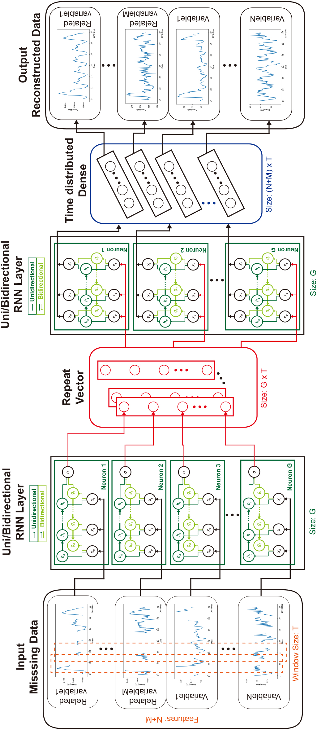
In the multi-feature implementation, each variable corresponds to a feature of the input. The time series is characterized by
Two widely used missing imputation methods, k-Nearest Neighbor Imputation (k-NN) [59] and Multiple Imputation by Chained Equation (MICE) [60], are used for comparing with the proposed RNN-DAE architecture. k-NN imputation method uses k-Nearest Neighbors algorithm for completing missing values in the dataset, which are imputed using the mean value from
The model validation can be divided into several steps. Data from three datasets are used. First, data preprocessing, which includes resampling and scaling of data, is then carried out. Then, a train-test split is performed. Additionally, input data is corrupted by introducing gaps in one or more variables, covering all possible combinations. Next, the models are trained and a cross-validation stage is performed to set the hyperparameters.
Then, the trained models are applied to the test data, which contains known missing data. The quality of reconstructed data is assessed using reconstruction error metrics, which provide insights into how well the models have captured the missing data. The performance is analyzed in different scenarios considering mean values of these errors, as well as the fitting and inference times. Last, scalability and efficiency are studied for specific situations, varying the corruption rate (gap length) and the number of variables with gaps, to determine the feasibility of deploying the best models in a real scenario. More detailed information about model validation and evaluation can be found in Section 4.
4.Experiments and results
4.1Experimental setup
Figure 2.
Electricity supply and submetering system (Module 10) at the Hospital of León.
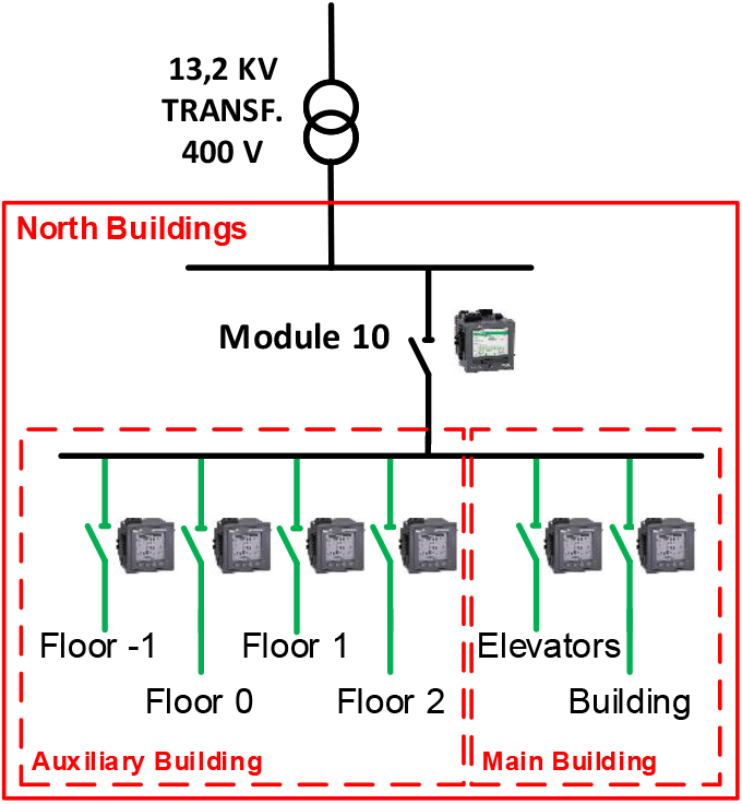
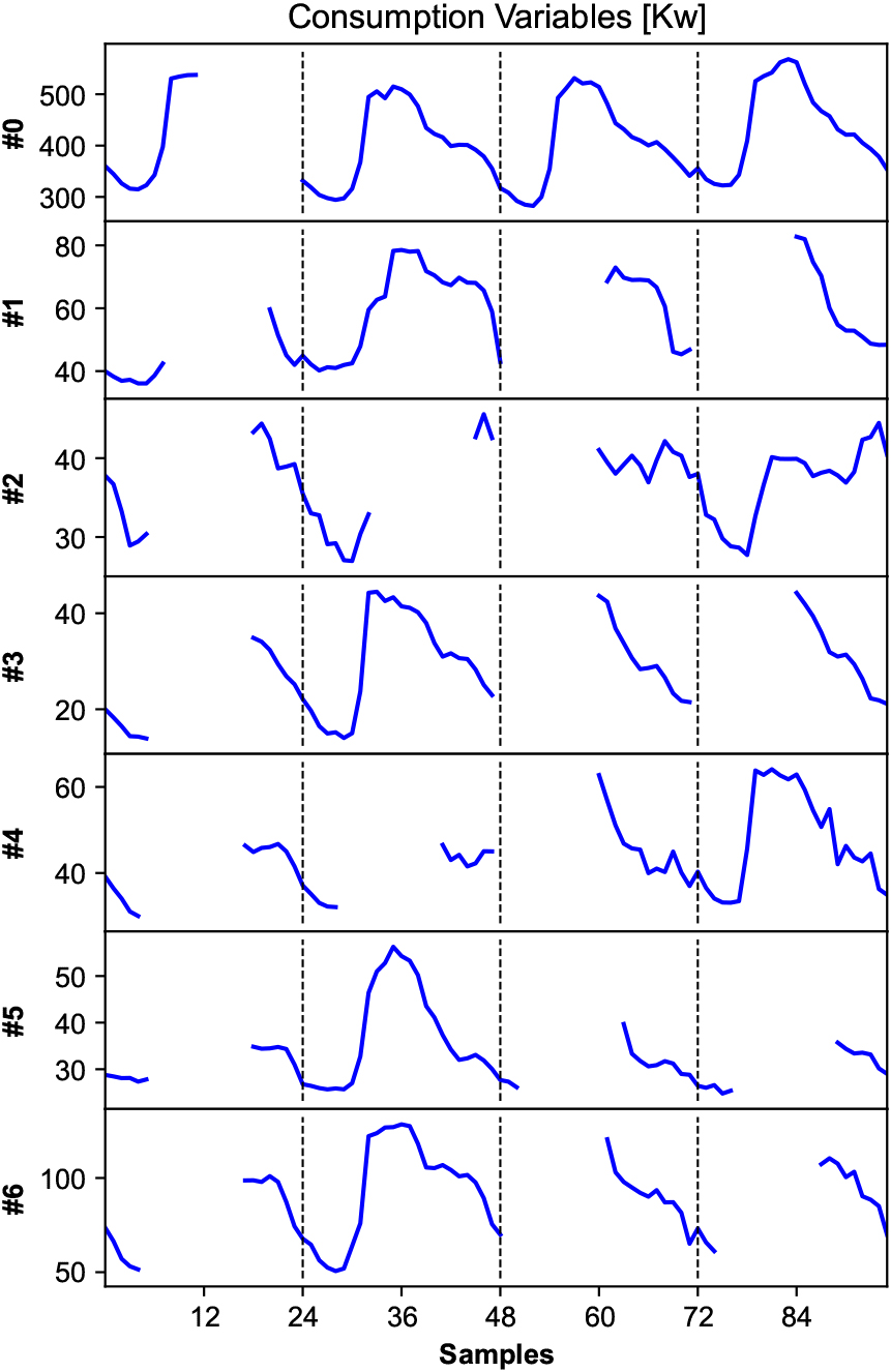
Three datasets have been used in the experiments. The first one, Hospital (Module 10) electricity consumption dataset, contains 508 daily load curves (electricity consumption for 24 hours) from 7 meters located at Module 10 of the submetering system at the Hospital of León. A schema is shown in Fig. 2, including the electricity supply and the submetering system. Module 10 serves as the electricity provider for the north buildings at the hospital, which include a main and an auxiliary building A transformer reduces voltage (13.2KV/400V) to supply electricity to 6 different zones in the north buildings. A main meter measures the overall electricity consumption of these north buildings. In addition, four submeters measure the electricity consumption of each floor in the auxiliary building. Other two submeters are installed in the main building to measure the electricity consumption of the elevators and other facilities in that building. All these meters measure electricity loads each 1 minute, but data are resampled to 1 hour to obtain the daily load curves. The values in the dataset range from 11 to 599 kilowatts. In Table 1, consumption variables corresponding to the mentioned 7 meters in the north buildings (Module 10) are listed.
Table 1
Consumption variables corresponding to meters located in the north buildings at the Hospital of León (Module 10)
| Id | Variable | Building |
|---|---|---|
| #0 | Overall consumption | North buildings |
| #1 | Consumption of floor | Auxiliary |
| #2 | Consumption of floor 0 | Auxiliary |
| #3 | Consumption of floor 1 | Auxiliary |
| #4 | Consumption of floor 2 | Auxiliary |
| #5 | Consumption of the elevators | Main |
| #6 | Consumption of the rest | Main |
In order to perform the experiments, the dataset was standardized in the [
The recurrent neural network-based denoising autoencoder requires noisy data as input, so empty values are intentionally introduced into the training subset. For that purpose, gaps are generated randomly by setting to
Gaps are also introduced into the test subset randomly, again by setting some values in the daily load curves to
Figure 3.
A pattern of gaps used in the test subset (Hospital dataset).
Additionally, to assess the range of applicability of the proposed approach, two public datasets are used in the experiments. UCI individual household electric power consumption dataset [61] contains measurements of electric power consumption in one household during a period of almost 4 years. The following variables were selected: Global active power and Submetering 1, 2 and 3. Data have been preprocessed and resampled at 1 hour intervals. Values range from 0 to 109 watts. On the other hand, REFIT electrical load measurements dataset [62] consists of cleaned electrical consumption data for 20 households at the aggregate level plus the consumption of 9 appliances (fridge, washing machine, dishwasher, microwave, television, etc.). For this study, data from house 18 (H18) during 1 year (starting in May 2014) were selected, preprocessed and resampled at 1 hour intervals. The values, in this case, range from 0 to 4960 watts.
Both the UCI and REFIT datasets were also standardized in the [
Table 2 summarizes the main characteristics of the three datasets used in this work.
Table 2
Description of the datasets
| Datasets | |||
| UCI | REFIT | Hospital | |
| [61] | (H18) [62] | (M10) | |
| Samples (24-long) | 1440 | 366 | 508 |
| Variables | 4 | 10 | 7 |
| Minimum value | 0.0 | 0.0 | 10.67 |
| Maximum value | 109.34 | 4960.54 | 599.46 |
| Units | Watts | Watts | Kilowatts |
A 10-fold cross-validation is carried out to tune the hyperparameters of the proposed method. The results from the cross-validation process determine the optimal number of neurons of each type of RNN (unidirectional and bidirectional ones). Considering that electricity consumption is generally periodic, the possible number of neurons ranges from 24 hours (1 day) to 168 hours (7 days). Test experiments are performed using the hyperparameters that yielded the best results in the validation step for each method and dataset.
The size of the training subsets (batch size) is set to 32 and input data are shuffled. The learning curves show that increasing the number of epochs produces overfitted models, so this parameter has been set to 8.
Table 3
Reconstruction errors (mean value) using state-of-the-art methods and datasets
| Methods | Datasets | ||||||
|---|---|---|---|---|---|---|---|
| UCI [61] | REFIT (H18) | Hospital (M10) | |||||
| [62] | |||||||
| RMSE | MAE | RMSE | MAE | RMSE | MAE | MAPE | |
| k-NN | 6.94 | 4.91 | 63.51 | 32.10 | 9.63 | 7.55 | 9.46 |
| MICE | 5.67 | 4.00 | 61.14 | 30.83 | 8.64 | 6.88 | 8.56 |
| SRNN-DAE | 5.63 | 3.63 | 59.07 | 25.32 | 6.77 | 4.99 | 6.28 |
| GRU-DAE | 5.61 | 3.61 | 58.20 | 26.08 | 5.41 | 4.22 | 5.47 |
| LSTM-DAE | 5.55 | 3.62 | 62.82 | 26.25 | 5.45 | 4.17 | 5.43 |
| BiSRNN-DAE | 5.57 | 3.68 | 60.69 | 25.82 | 5.38 | 4.09 | 5.60 |
| BiGRU-DAE | 5.33 | 3.34 | 61.40 | 26.51 | 5.07 | 3.82 | 5.21 |
| BiLSTM-DAE | 5.42 | 3.35 | 61.94 | 26.56 | 5.47 | 4.12 | 5.47 |
Table 4
Fitting and inference times
| Methods | Datasets | |||||||||||
|---|---|---|---|---|---|---|---|---|---|---|---|---|
| UCI [61] | REFIT (H18) [62] | Hospital (M10) | ||||||||||
| Fitting [s] | Inference [s] | Fitting [s] | Inference [s] | Fitting [s] | Inference [s] | |||||||
| k-NN | 0. | 01 | 2249. | 86 | 0. | 09 | 1316039 | 0. | 04 | 26065. | 34 | |
| MICE | 1. | 63 | 0. | 12 | 144. | 12 | 7. | 92 | 11. | 94 | 0. | 72 |
| SRNN-DAE | 44. | 64 | 1. | 40 | 706. | 11 | 19. | 27 | 122. | 19 | 3. | 42 |
| GRU-DAE | 77. | 24 | 2. | 15 | 1235. | 34 | 35. | 41 | 215. | 32 | 5. | 44 |
| LSTM-DAE | 122. | 44 | 3. | 21 | 2018. | 51 | 66. | 68 | 341. | 15 | 8. | 22 |
| BiSRNN-DAE | 55. | 29 | 1. | 88 | 856. | 20 | 28. | 28 | 148. | 68 | 4. | 63 |
| BiGRU-DAE | 199. | 60 | 3. | 74 | 3209. | 82 | 87. | 12 | 556. | 24 | 9. | 44 |
| BiLSTM-DAE | 248. | 77 | 4. | 68 | 3659. | 56 | 95. | 43 | 669. | 07 | 12. | 07 |
In the case of the k-NN, the number of neighbors is chosen to be
The experiments have been executed on a PC equipped with an Intel Core i7-6700 3.40GHz CPU and 16GB RAM. No GPU memory is used. The implementation was done using Python 3.6.7 programming language and the following libraries Keras 2.2.2 [63], Tensorflow 1.12 [64] and scikit-learn 0.20.1 [65].
Reconstruction errors are computed only based on missing samples. Root Mean Square Error (RMSE), Mean Absolute Error (MAE) and Mean Absolute Percentage Error (MAPE) have been chosen as evaluation metrics. Note that both UCI and REFIT datasets contain many zero values (35% and 31%, respectively), so that MAPE error would be undefined and, therefore, will not be computed.
4.2Results
The first experiment compares the mean reconstruction errors of the state-of-the-art and proposed approaches as a global metric for the overall submetering system in the three datasets. Table 3 shows the results obtained in each case. Additionally, computational times for both training and test subsets are presented in Table 4 as a secondary measure for the comparison.
The proposed method with BiGRU layers (BiGRU-DAE) achieved the lowest errors (highlighted in bold) using two datasets (UCI and Hospital). According to the mean values shown in Table 3, BiGRU-DAE provides a RMSE of 5.33 and a MAE of 3.34 for the UCI dataset, and it gives the following errors when using the Hospital dataset: 5.07 (RMSE), 3.82 (MAE), and 5.21 (MAPE). On the contrary, the proposed method with GRU and SRNN layers obtained the best values for the REFIT dataset. GRU-DAE provides the lowest RMSE (58.20), whereas SRNN-DAE gives the lowest MAE (25.32). In order to choose one of these two recurrent layers for the proposed method using the REFIT dataset, fitting and inference times could also be considered. As you can see in Table 4, SRNN is slightly faster than GRU in both the fitting and inference phases (1.75 and 1.84 times faster, respectively). It is worth noting that bidirectional RNNs generally take more time due to the need to process input data in both the forward and backward directions. Therefore, BiGRU-DAE and SRNN-DAE will be used in a further analysis of the results. However, GRU-DAE has also proven to give outstanding reconstruction errors.
Table 5
Reconstruction errors for each variable of the best-performing method in each dataset
| Methods | Errors | Variable Id | |||||||||
| #0 | #1 | #2 | #3 | #4 | #5 | #6 | #7 | #8 | #9 | ||
| UCI dataset [61] | |||||||||||
| BiGRU-DAE | RMSE | 8.93 | 3.17 | 3.74 | 5.50 | – | – | – | – | – | – |
| MAE | 6.26 | 1.62 | 1.60 | 3.88 | – | – | – | – | – | – | |
| REFIT (H18) dataset [62] | |||||||||||
| SRNN-DAE | RMSE | 252.57 | 22.76 | 31.81 | 19.40 | 30.56 | 44.86 | 122.57 | 18.72 | 17.98 | 29.42 |
| MAE | 136.17 | 12.47 | 17.97 | 13.42 | 8.18 | 13.56 | 26.53 | 9.36 | 10.37 | 5.17 | |
| Hospital (M10) dataset | |||||||||||
| BiGRU-DAE | RMSE | 14.79 | 6.55 | 1.82 | 1.88 | 3.33 | 1.73 | 5.39 | – | – | – |
| MAE | 10.79 | 4.96 | 1.43 | 1.39 | 2.63 | 1.35 | 4.19 | – | – | – | |
| MAPE | 2.85 | 8.28 | 4.19 | 5.71 | 6.61 | 4.02 | 4.81 | – | – | – | |
These results reveal two findings: first, bidirectional RNNs provide similar or slightly lower errors than unidirectional RNNs for the extraction of temporal information and relations among variables in this data reconstruction problem; second, considering data both before and after the gap and introducing GRU (unidirectional or bidirectional) in the hidden layers of a denoising autoencoder (DAE) results in a useful architecture for missing data imputation in related multivariate time series.
Comparing the state-of-the-art methods (kNN and MICE) with the proposed approach, it can be seen that k-NN yields the worst performance (RMSE, MAE and MAPE) using the three datasets. It also has a very high computational cost in the inference phase whenever the dataset is large (e.g., k-NN required several days for the REFIT dataset). On the other hand, MICE provides slightly higher errors (except for the RMSE in the REFIT dataset) but, in turn, is the fastest data imputation method.
In order to analyze the performance reported in Table 3 in further detail, Table 5 presents the reconstruction errors for each variable of the best-performing methods in the three datasets, i.e., BiGRU-DAE and SRNN-DAE. For all datasets, variable id. #0 corresponds to the aggregated power consumption value, and the remaining ones (#1–#9) are the variables of the lower metering level.
For the UCI dataset, BiGRU-DAE yields the lowest errors in variables id. #1 and #2, corresponding to the consumption at the kitchen and the laundry room. On the contrary, aggregated consumption (#0), together with the consumption of the water-heater and the air-conditioner (#3), presents the highest errors.
For the REFIT dataset, variables id. #0 (Aggregated) and #6 (Dishwasher) have the highest RMSE (252.57 and 122.57, respectively) and MAE (136.17 and 26.53, respectively) errors when using SRNN-DAE, whereas the remaining variables are reconstructed by SRNN-DAE with low errors. RMSE ranges from 17.98 (#8-TV) to 44.86 (#5-Washing machine) and MAE varies from 5.17 (#9-Microwave) to 17.97 (#2-Freezer).
For the Hospital (M10) dataset, BiGRU-DAE yields the highest RMSE and MAE errors in four variables (#0, #1, #4, #6). RMSE fluctuates from 14.79 (#0-Aggregated) to 3.33 (#4-Floor 2) and MAE ranges from 10.79 (#0-Aggregated) to 2.63 (#4-Floor 2). On the contrary, BiGRU-DAE provides low values in three variables (#2, #3, #5), ranging the RMSE from 1.88 (#3-Floor 1) to 1.73 (#5-Elevators) and MAE from 1.43 (#2-Floor 0) to 1.35 (#5-Elevators). Variable #0 (Aggregated) can be reconstructed by the BiGRU-DAE with a MAPE of 2.85 while variables #1 (Floor
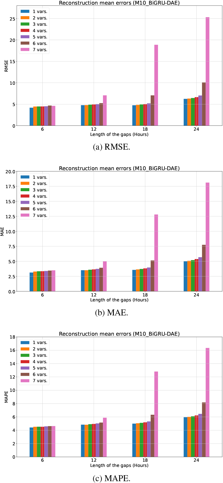
Finally, in order to understand the behavior of the proposed approach under different scenarios, we have conducted experiments where the corruption rate and the number of variables containing gaps are controlled parameters. Figures 4–6 show the results obtained from the best performing methods, BiGRU-DAE and SRNN-DAE, using the UCI, REFIT and Hospital datasets, under different scenarios. Using the corresponding test subsets, mean errors for the overall submetering system are computed considering four specific corruption rates (25%-6 hours, 50%-12 hours, 75%-18 hours, 100%-24 hours) and a varying number of variables with gaps (from 1 to all variables which contain each dataset), regardless of which variables are included. This approach allows for the examination of multiple data loss scenarios and a better understanding of the performance of the proposed method.
Figure 4.
Reconstruction errors (mean value) using BiGRU-DAE in the UCI dataset.
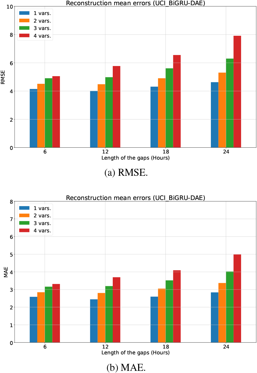
Figure 5.
Reconstruction errors (mean value) using SRNN-DAE in the REFIT (H18) dataset.
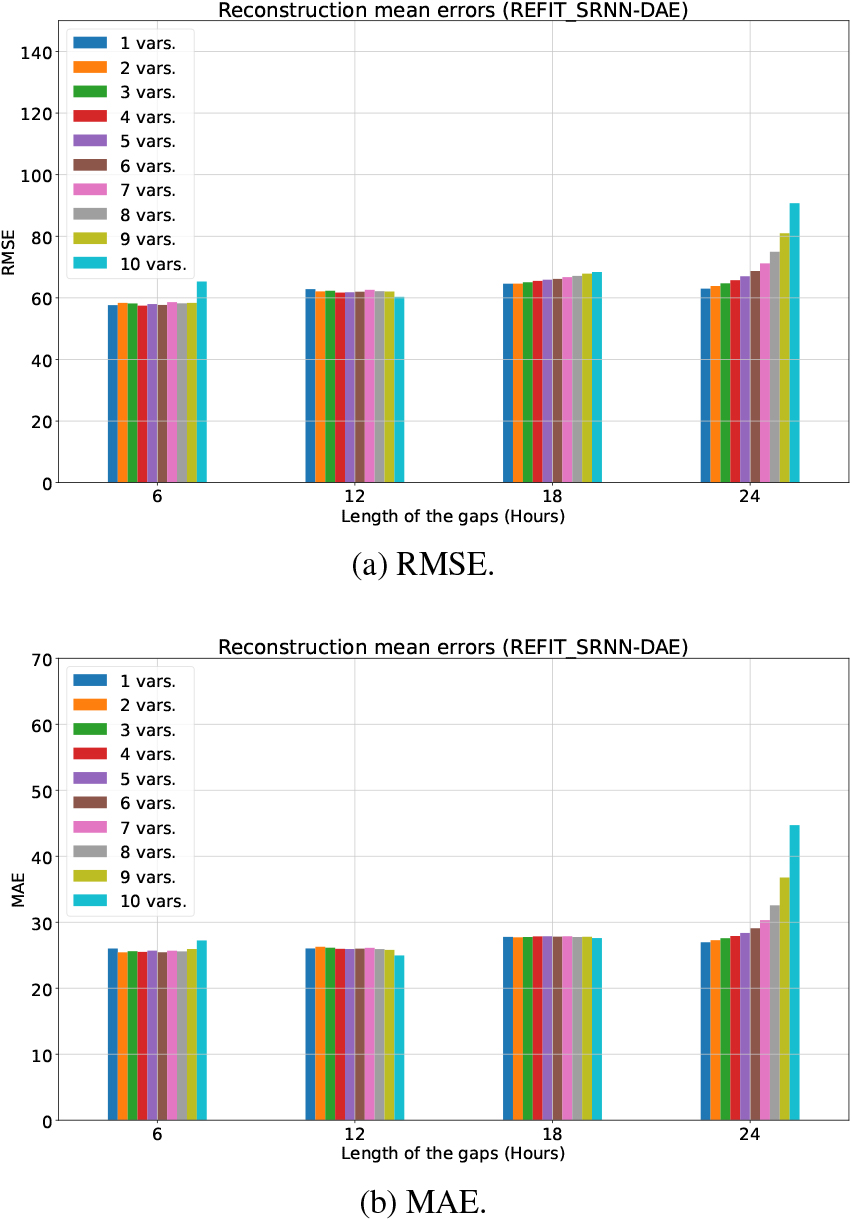
Figure 6.
Reconstruction errors (mean value) using BiGRU-DAE in the Hospital (M10) dataset.
For the UCI dataset, a total of 16 different scenarios are studied, corresponding to four gap lengths (6, 12, 18 and 24 hours) and the number of variables with gaps (from 1 to 4 variables). Figure 4 shows the reconstruction errors (RMSE and MAE), using bidirectional GRUs in the hidden layers of DAE (BiGRU-DAE). At a glance, similar errors (RMSE and MAE) are obtained for the four different gap lengths. However, as expected, both RMSE and MAE are higher for corruption rates of 75% and 100%, regardless of the number of variables with missing samples. Furthermore, it should be pointed out that RMSE and MAE errors for a corruption rate of 25% (a gap length of 6 hours) are slightly higher than errors for a corruption rate of 50% (a gap length of 12 hours). Although counter-intuitive, it is likely due to the great number of zeros this dataset has in the submetering variables, because longer gaps with more zeros will be easier to impute. It can be seen that the more variables contain missing samples, the higher RMSE and MAE errors are. Nevertheless, BiGRU-DAE is able to impute gaps successfully (being RMSE and MAE errors lower than 8 and 5, respectively) if all variables comprise missing samples, even for a corruption rate of 100%.
For the REFIT dataset, a total of 1024 different scenarios are studied, corresponding to four gap lengths (6, 12, 18 and 24 hours) and the varying number of variables with gaps (from 1 to 10 variables). Figure 5 shows the reconstruction errors (RMSE and MAE) using unidirectional simple RNNs in the hidden layers of DAE (SRNN-DAE). As expected, RMSE error increases for the four different gap lengths, regardless of the number of variables with missing samples. On the contrary, the MAE error for a corruption rate of 25% (a gap length of 6 hours) is higher or equal than the one for a corruption rate of 50% (a gap length of 12 hours). This dataset also comprises a great number of zeros related to the consumption of appliances, so that shorter gaps with few zeros will be harder to impute. It should be highlighted that RMSE and MAE errors provided by SRNN-DAE are stable when the corruption rate is 50% and 75%, independently of the number of variables with missing samples. Moreover, errors are even lower when the 10 variables comprise missing samples (a gap length of 12 hours). On the contrary, when the corruption rate is 100%, both errors increase exponentially with the number of variables comprising missing samples. SRNN-DAE performs successfully the gap imputation (being RMSE and MAE errors lower than 70 and 30, respectively), except if all or many variables comprise missing samples for a corruption rate of 100%.
For the Hospital dataset, a total of 28 different scenarios are studied, corresponding to four gap lengths (6, 12, 18 and 24 hours) and the number of variables with gaps (from 1 to 7 variables). Figure 6 shows the reconstruction errors (RMSE, MAE and MAPE) using bidirectional GRUs in the hidden layers of DAE (BiGRU-DAE). It can be seen that the lowest errors (RMSE, MAE and MAPE) are achieved with a gap length of 6 hours (corruption rate of 25%) regardless of the number of variables containing missing samples. In this case, data can be reconstructed with certain of accuracy, as the errors are limited. As expected, the longer the gap length is, the higher reconstruction errors are, especially if many variables include gaps simultaneously. However, errors are reasonably stable for gap lengths of 12 and 18 hours (corruption rates of 50% and 75%), except in the case where all variables contain gaps (in this case, the errors increase notably). Even for a gap length of 24 hours (corruption rate of 100%), BiGRU-DAE is able to fill gaps with errors lower or equal than 10, but it requires that at least one variable contains complete data. However, if all variables have gaps, the errors rise sharply, revealing BiGRU-DAE is not able to reconstruct data in this adverse scenario.
5.Discussion
Summarizing the results, denoising autoencoders (DAEs) are able to recreate satisfactorily input missing data, filling the gaps deliberately added to the input data. Indeed, the use of recurrent layers outperforms previous methods such as K-NN and MICE. Furthermore, GRUs are found to be interesting recurrent neural networks for capturing temporal patterns in time series. Compared to other RNNs, GRUs are simpler, have shorter training and inference times, require fewer parameters adjustments, and provide better results. Only simple RNNs could achieve comparable results with shorter times for a specific dataset. The introduction of bidirectional GRUs improves the results by leveraging data both before and after the gap. However, it increases the computational cost and times compared to unidirectional GRU.
In the adverse scenario where most or all variables contain long gaps, the proposed approach is not able to reconstruct data with accuracy due to the absence of past or future information and the limited possibility of establishing connection among variables. In scenarios where no data are available, the reconstruction problem should then be reformulated as a prediction problem, considering regressor variables and periodicity. On the other extreme, applying the proposed approach in a friendlier, much simpler scenario, e.g., with a gap length of 1 hour in one or a few variables, is not advisable, since simpler methods such as a linear interpolation would competently solve this straightforward problem.
Thus, the proposed approach based on a denoising autoencoder (DAE) with unidirectional GRU (GRU-DAE), simple RNN (SRNN-DAE) or bidirectional GRU layers (BiGRU-DAE) is promising for imputing missing samples and reconstructing related multivariate time series in a wide range of scenarios. In this work, three varied datasets comprising electricity consumption variables have been used. Electricity consumption in households is mainly due to appliances which are controlled using an on-off switching mode. Therefore, these consumption profiles are irregular with two defined states and contain zeros. On the contrary, consumption variables in large buildings present gradual changes (increases or decreases) with minimum values greater than zero and the relationships among variables are closer, so missing samples are easier to impute. The proposed method could also be applied to fill gaps in multiple domains.
The multi-feature implementation, comprising an uni- or bidirectional GRU encoding the features (variables) and another uni- or bidirectional GRU decoding the encoded vector, and thus providing complete output data, possesses a bounded computational cost when the number of variables is high. On the other hand, the drawbacks of the proposed approach are, in short: that it requires complete data for training; its acceptable, but still not negligible, computational cost when bidirectional RNNs are used; and that it is not recommended in extreme scenarios, in which other approaches could perform better.
Considering related works, missing imputation performance was evaluated in [13] for daily load profiles of residential data, where a DAE model showed better results than other models such as linear interpolation, historical average or variational and Wasserstein autoencoders. Feedforward, convolutional and LSTM autoencoders were also analyzed for the reconstruction of indoor environment [46]. They outperformed polynomial interpolation and the best results were shown by the LSTM architecture for non-corrupted and forecasting data, but the convolutional configuration was the best one for reconstructing sub-daily data gaps. In our case, the comparison is performed using DAE with different recurrent layers including bidirectional networks that help to capture temporal relationships by considering both forward and backward information.
Bidirectional RNN as generative models were proposed [50] for time series with probabilistic approaches using text data, showing their effectiveness in cases where Bayesian inference of a unidirectional RNN was impracticable. The robustness of simple, convolutional and Bi-LSTM autoencoders was also considered, with Bi-LSTM showing the best performance even with a high missing rate, despite its higher computational cost. A long interval gap-filling model, BiLSTM-I [11], was applied to meteorological temperature observation data reaching high accuracy for half-hourly temperature observations including imputation error into the model convergence. It uses a bidirectional LSTM in the encoder and a unidirectional LSTM in the decoder. These works demonstrated the suitability of bidirectional architectures in other domains, especially in challenging cases with high rates of missing data or irregular values of the variables.
6.Conclusions
In this paper, an approach (RNN-DAE) is proposed for gap imputation in related multivariate time series, specifically in the context of energy submetering. The approach uses a denoising autoencoder (DAE) architecture with recurrent neural networks (RNNs) in the hidden layers. The DAE is in charge of filling input missing data, removing the gaps added intentionally to the input data as noise. The RNN aims to capture temporal patterns and relationships among variables in the time series. Various recurrent neural networks have been assessed in the experiments, including unidirectional models such as Simple RNN, GRU, and LSTM, as well as bidirectional models like BiSRNN, BiGRU, and BiLSTM. The use of bidirectional RNNs allows for the consideration of data both before and after the gap, unlike unidirectional models.
The experiments used three different datasets, a real dataset comprising 7 related electricity consumption variables from the Hospital of León, as well as two public datasets comprising consumption variables. For that purpose, daily load curves (24 samples long) have been built. A multi-feature implementation of the proposed approach with unidirectional GRUs (GRU-DAE) or simple RNNs (SRNN-DAE) has proven to be an outstanding method for filling potential gaps in the daily load curves. The implementation with bidirectional GRU layers (BiGRU-DAE) has also provided excellent results, albeit with increased computational cost.
The proposed approach with bidirectional GRU layers (BiGRU-DAE) is able to fill gaps efficiently with low reconstruction errors in a wide range of scenarios. It is able to reconstruct related multivariate time series with high corruption rates (up to 75%), as long as at least one of the variables contains complete data. The performance of the proposed approach is consistently better than the ones obtained by MICE and k-NN.
The use of this approach is appropriate in complex scenarios, in which there are several variables containing long gaps, because its application in straightforward scenarios (very short gaps in one variable) is unnecessary. Additionally, the approach should not be applied in extremely adverse scenarios where no data from any variable are available, as it lacks prediction capabilities.
As future work, the introduction of nonlinear activation functions and additional stacked layers could be explored in order to consider latent relations among variables. One-dimensional CNNs are promising alternatives, especially separable CNNs that align with the structure of related multivariate time series. Furthermore, the impact of the gap position in the time series (at the beginning, in the middle or at the end) should be studied in detail. The performance of the proposed approach should also be analyzed with long sequences of input data, longer than 24 hours or sampled at higher rates. Finally, the consideration of alternative machine learning techniques, including ensemble learning or self-supervised learning, can be interesting to address the problem.
Funding
Grant PID2020-117890RB-I00 funded by MCIN/ AEI/10.13039/ 501100011033.
References
[1] | Klingenberg CO, Borges MAV, Antunes JAV Jr. Industry 4.0 as a data-driven paradigm: A systematic literature review on technologies. Journal of Manufacturing Technology Management. (2021) ; 32: (3): 570–592. doi: 10.1108/JMTM-09-2018-0325. |
[2] | Yan J, Meng Y, Lu L, Li L. Industrial Big Data in an Industry 4.0 Environment: Challenges, schemes, and applications for predictive maintenance. IEEE Access. (2017) ; 5: : 23484–23491. doi: 10.1109/ACCESS.2017.2765544. |
[3] | Teh HY, Kempa-Liehr AW, Wang KI-K Sensor data quality: A systematic review. Journal of Big Data. (2020) ; 7: (1). doi: 10.1186/s40537-020-0285-1. |
[4] | Ahmad T. Non-technical loss analysis and prevention using smart meters. Renewable and Sustainable Energy Reviews. (2017) ; 72: : 573–589. |
[5] | Deb C, Zhang F, Yang J, Lee SE, Shah KW. A review on time series forecasting techniques for building energy consumption. Renewable and Sustainable Energy Reviews. (2017) ; 74: : 902–924. |
[6] | Li D, Li L, Li X, Ke Z, Hu Q. Smoothed LSTM-AE: A spatio-temporal deep model for multiple time-series missing imputation. Neurocomputing. (2020) ; 411: : 351–363. |
[7] | Little RJA, Rubin DB. Statistical analysis with missing data (Vol. 793). John Wiley & Sons. (2019) . |
[8] | Liang Y, Zhao Z, Sun L. Memory-augmented dynamic graph convolution networks for traffic data imputation with diverse missing patterns. Transportation Research Part C: Emerging Technologies. (2022) ; 143: : 103826. doi: 10.1016/j.trc.2022.103826. |
[9] | Parrella ML, Albano G, La Rocca M, Perna C. Reconstructing missing data sequences in multivariate time series: An application to environmental data. Statistical Methods & Applications. (2019) ; 28: (2): 359–383. doi: 10.1007/s10260-018-00435-9. |
[10] | Al-Wakeel A, Wu J, Jenkins N. K-means based load estimation of domestic smart meter measurements. Applied Energy. (2017) ; 194: , 333–342. |
[11] | Xie C, Huang C, Zhang D, He W. BiLSTM-I: A deep learning-based long interval gap-filling method for meteorological observation data. International Journal of Environmental Research and Public Health. (2021) ; 18: (19): 10321. |
[12] | Cao W, Wang D, Li J, Zhou H, Li L, Li Y. Brits: Bidirectional recurrent imputation for time series. Advances in Neural Information Processing Systems. (2018) ; 31: . |
[13] | Ryu S, Kim M, Kim H. Denoising autoencoder-based missing value imputation for smart meters. IEEE Access. (2020) ; 8: : 40656–40666. |
[14] | Alonso S, Morán A, Pérez D, Prada MA, Fuertes JJ, Domínguez M. Reconstructing Electricity Profiles in Submetering Systems Using a GRU-AE Network. In L. Iliadis, C. Jayne, A. Tefas and E. Pimenidis (Eds.), Engineering Applications of Neural Networks. Cham: Springer International Publishing. (2022) . pp. 247–259. doi: 10.1007/978-3-031-08223-8_21. |
[15] | Avola D, Cascio M, Cinque L, Foresti GL, Pannone D. Machine learning for video event recognition. Integrated Computer-Aided Engineering. (2021) ; 28: (3): 309–332. |
[16] | Martins GB, Papa JP, Adeli H. Deep learning techniques for recommender systems based on collaborative filtering. Expert Systems. (2020) ; 37: (6): 12647. |
[17] | Oh BK, Yoo SH, Park HS. A measured data correlation-based strain estimation technique for building structures using convolutional neural network. Integrated Computer-Aided Engineering. (2023) ; 30: (4): 395–412. doi: 10.3233/ICA-230714. |
[18] | Alonso S, Morán A, Pérez D, Prada MA, Fuertes JJ, Domínguez M. Virtual sensor for probabilistic estimation of the evaporation in cooling towers. Integrated Computer-Aided Engineering. (2021) ; 28: (4): 369–381. |
[19] | Alahakoon D, Yu X. Smart electricity meter data intelligence for future energy systems: A survey. IEEE Transactions on Industrial Informatics. (2016) ; 12: (1): 425–436. doi: 10.1109/TII.2015.2414355. |
[20] | Wang Y, Chen Q, Hong T, Kang C. Review of smart meter data analytics: Applications, methodologies, and challenges. IEEE Transactions on Smart Grid. (2018) ; 10: (3): 3125–3148. |
[21] | Miraftabzadeh SM, Longo M, Foiadelli F, Pasetti M, Igual R. Advances in the application of machine learning techniques for power system analytics: A survey. Energies. (2021) ; 14: (16): 4776. |
[22] | Chicco G. Overview and performance assessment of the clustering methods for electrical load pattern grouping. Energy. (2012) ; 42: (1): 68–80. |
[23] | Al-Wakeel A, Wu J, Jenkins N. State estimation of medium voltage distribution networks using smart meter measurements. Applied Energy. (2016) ; 184: : 207–218. |
[24] | Yang S-l, Shen C, et al. A review of electric load classification in smart grid environment. Renewable and Sustainable Energy Reviews. (2013) ; 24: : 103–110. |
[25] | Glauner P, Meira JA, Valtchev P, Bettinger F, et al. The challenge of non-technical loss detection using artificial intelligence: A survey. International Journal of Computational Intelligence Systems. (2017) ; 10: (1): 760. |
[26] | Duchesne L, Karangelos E, Wehenkel L. Recent developments in machine learning for energy systems reliability management. Proceedings of the IEEE. (2020) ; 108: (9): 1656–1676. |
[27] | Fu Y, Li Z, Zhang H, Xu P. Using support vector machine to predict next day electricity load of public buildings with sub-metering devices. Procedia Engineering. (2015) ; 121: : 1016–1022. doi: 10.1016/j.proeng.2015.09.097. |
[28] | Ji Y, Xu P, Duan P, Lu X. Estimating hourly cooling load in commercial buildings using a thermal network model and electricity submetering data. Applied Energy. (2016) ; 169: : 309–323. doi: 10.1016/j.apenergy.2016.02.036. |
[29] | Morán A, Alonso S, Pérez D, Prada MA, Fuertes JJ, Domínguez M. Feature extraction from building submetering networks using deep learning. Sensors. (2020) ; 20: (13). doi: 10.3390/s20133665. |
[30] | Hart GW. Nonintrusive appliance load monitoring. Proceedings of the IEEE. (1992) ; 80: (12): 1870–1891. |
[31] | Zeifman M, Roth K. Nonintrusive appliance load monitoring: Review and outlook. IEEE Transactions on Consumer Electronics. (2011) ; 57: (1): 76–84. |
[32] | Zoha A, Gluhak A, Imran MA, Rajasegarar S. Non-intrusive load monitoring approaches for disaggregated energy sensing: A survey. Sensors. (2012) ; 12: (12): 16838–16866. |
[33] | Kelly J, Knottenbelt W. Neural nilm: Deep neural networks applied to energy disaggregation. In Proceedings of the 2nd ACM International Conference on Embedded Systems for Energy-Efficient Built Environments. (2015) . pp. 55–64. |
[34] | García-Pérez D, Pérez-López D, Díaz-Blanco I, González-Muñiz A, Domínguez-González M, Cuadrado Vega AA. Fully-convolutional denoising auto-encoders for NILM in large non-residential buildings. IEEE Transactions on Smart Grid. (2021) ; 12: (3), 2722–2731. doi: 10.1109/TSG.2020.3047712. |
[35] | Lara-Benítez P, Carranza-García M, Riquelme JC. An experimental review on deep learning architectures for time series forecasting. International Journal of Neural Systems. (2021) ; 31: (03): 2130001. |
[36] | Chandra R, Goyal S, Gupta R. Evaluation of deep learning models for multi-step ahead time series prediction. IEEE Access. (2021) ; 9: : 83105–83123. doi: 10.1109/ACCESS.2021.3085085. |
[37] | Torres JF, Galicia A, Troncoso A, Martínez-Álvarez F. A scalable approach based on deep learning for big data time series forecasting. Integrated Computer-Aided Engineering. (2018) ; 25: (4): 335–348. |
[38] | Fan C, Wang J, Gang W, Li S Assessment of deep recurrent neural network-based strategies for short-term building energy predictions. Applied Energy. (2019) ; 236: : 700–710. doi: 10.1016/j.apenergy.2018.12.004. |
[39] | Kong W, Dong ZY, Jia Y, Hill DJ, Xu Y, Zhang Y. Short-term residential load forecasting based on LSTM recurrent neural network. IEEE Transactions on Smart Grid. (2017) ; 10: (1): 841–851. |
[40] | Gupta A, Gurrala G, Sastry PS. Instability Prediction in Power Systems using Recurrent Neural Networks. In IJCAI. (2017) . pp. 1795–1801. |
[41] | Lee S, Jin H, Nengroo SH, Doh Y, Lee C, Heo T, Har D. Smart Metering System Capable of Anomaly Detection by Bi-directional LSTM Autoencoder. In 2022 IEEE International Conference on Consumer Electronics (ICCE). (2022) . pp. 1–6. |
[42] | Perez-Ramirez CA, Amezquita-Sanchez JP, Valtierra-Rodriguez M, Adeli H, Dominguez-Gonzalez A, Romero-Troncoso RJ. Recurrent neural network model with Bayesian training and mutual information for response prediction of large buildings. Engineering Structures. (2019) ; 178: : 603–615. |
[43] | Pereira RC, Santos MS, Rodrigues PP, Abreu PH. Reviewing autoencoders for missing data imputation: Technical trends, applications and outcomes. Journal of Artificial Intelligence Research. (2020) ; 69: : 1255–1285. |
[44] | Noering FK-D, Schroeder Y, Jonas K, Klawonn F. Pattern discovery in time series using autoencoder in comparison to nonlearning approaches. Integrated Computer-Aided Engineering. (2021) ; 28: (3): 237–256. |
[45] | Jiang K, Han Q, Du X, Ni P. A decentralized unsupervised structural condition diagnosis approach using deep auto-encoders. Computer-Aided Civil and Infrastructure Engineering. (2021) ; 36: (6): 711–732. |
[46] | Liguori A, Markovic R, Dam TTH, Frisch J, van Treeck C, Causone F. Indoor environment data time-series reconstruction using autoencoder neural networks. Building and Environment. (2021) a; 191: : 107623. doi: 10.1016/j.buildenv.2021.107623. |
[47] | Liguori A, Markovic R, Frisch J, Wagner A, Causone F, van Treeck C. A gap-filling method for room temperature data based on autoencoder neural networks. In Proceedings of Building Simulation 2021: 17th Conference of IBPSA. Building Simulation. Bruges, Belgium: IBPSA. Vol. 17, (2021) b. pp. 2427–2434. doi: 10.26868/25222708.2021.30232. |
[48] | Abiri N, Linse B, Edén P, Ohlsson M. Establishing strong imputation performance of a denoising autoencoder in a wide range of missing data problems. Neurocomputing. (2019) ; 365: : 137–146. |
[49] | Lai X, Wu X, Zhang L, Lu W, Zhong C. Imputations of missing values using a tracking-removed autoencoder trained with incomplete data. Neurocomputing. (2019) ; 366: : 54–65. |
[50] | Berglund M, Raiko T, Honkala M, Kärkkäinen L, Vetek A, Karhunen JT. Bidirectional recurrent neural networks as generative models. Advances in Neural Information Processing Systems. (2015) ; 28: . |
[51] | Kaufmann M, Aksan E, Song J, Pece F, Ziegler R, Hilliges O. Convolutional autoencoders for human motion infilling. In 2020 International Conference on 3D Vision (3DV). IEEE. (2020) . pp. 918–927. |
[52] | Daniels J, Bailey CP, Liang L. Filling Cloud Gaps in Satellite AOD Retrievals Using an LSTM CNN-Autoencoder Model. In IGARSS 2022-2022 IEEE International Geoscience and Remote Sensing Symposium. IEEE. (2022) . pp. 2758–2761. |
[53] | Jiang B, Siddiqi MD, Asadi R, Regan A. Imputation of missing traffic flow data using denoising autoencoders. Procedia Computer Science. (2021) ; 184: : 84–91. |
[54] | Vincent P, Larochelle H, Lajoie I, Bengio Y, Manzagol P-A. Stacked denoising autoencoders: Learning useful representations in a deep network with a local denoising criterion. Journal of Machine Learning Research. (2010) ; 11: : 3371–3408. |
[55] | Rumelhart D, Hinton G, Williams R. Learning representations by back-propagating errors. Nature. (1986) ; 323: : 533–536. |
[56] | Cho K, van Merrienboer B, Gulcehre C, Bahdanau D, Bougares F, Schwenk H, Bengio Y. Learning Phrase Representations using RNN Encoder-Decoder for Statistical Machine Translation. arXiv preprint. (2014) . doi: 10.48550/ARXIV.1406.1078. |
[57] | Hochreiter S, Schmidhuber J. Long short-term memory. Neural Computation. (1997) ; 9: (8): 1735–1780. doi: 10.1162/neco.1997.9.8.1735. |
[58] | Yang S, Yu X, Zhou Y. LSTM and GRU Neural Network Performance Comparison Study: Taking Yelp Review Dataset as an Example. In 2020 International Workshop on Electronic Communication and Artificial Intelligence (IWECAI). (2020) . pp. 98–101. doi: 10.1109/IWECAI50956.2020.00027. |
[59] | Troyanskaya O, Cantor M, Sherlock G, Brown P, Hastie T, Tibshirani R, Botstein D, Altman RB. Missing value estimation methods for DNA microarrays. Bioinformatics. (2001) ; 17: (6): 520–525. doi: 10.1093/bioinformatics/17.6.520. |
[60] | Azur MJ, Stuart EA, Frangakis C, Leaf PJ. Multiple imputation by chained equations: What is it and how does it work? International Journal of Methods in Psychiatric Research. (2011) ; 20: (1): 40–49. doi: 10.1002/mpr.329. |
[61] | Hebrail G, Berard A. Individual household electric power consumption. UCI Machine Learning Repository. (2012) . doi: 10.24432/C58K54. |
[62] | Murray D, Stankovic L, Stankovic V. An electrical load measurements dataset of United Kingdom households from a two-year longitudinal study. Scientific Data. (2017) ; 4: (1): 160122. doi: 10.1038/sdata.2016.122. |
[63] | Chollet F, et al. Keras. (2015) . https://keras.io. |
[64] | Abadi M, Agarwal A, et al. TensorFlow: Large-Scale Machine Learning on Heterogeneous Systems. Software available from tensorflow.org. (2015) . https://www.tensorflow.org/. |
[65] | Pedregosa F, Varoquaux G, Gramfort A, Michel V, Thirion B, Grisel O, Blondel M, Prettenhofer P, Weiss R, Dubourg V, Vanderplas J, Passos A, Cournapeau D, Brucher M, Perrot M, Duchesnay E. Scikit-learn: Machine learning in python. Journal of Machine Learning Research. (2011) ; 12: : 2825–2830. |


