Neuro-distributed cognitive adaptive optimization for training neural networks in a parallel and asynchronous manner

Michailidis, Panagiotis; Michailidis, Iakovos T.; Gkelios, Sokratis; Karatzinis, Georgios; Kosmatopoulos, Elias B.

doi:10.3233/ICA-230718

Neuro-distributed cognitive adaptive optimization for training neural networks in a parallel and asynchronous manner

Article type: Research Article

Authors: Michailidis, Panagiotis^{a; b} | Michailidis, Iakovos T.^{a; b} | Gkelios, Sokratis^{a; b} | Karatzinis, Georgios^{a; b} | Kosmatopoulos, Elias B.^{a; b; *}

Affiliations: [a] Department of Electrical and Computer Engineering, Democritus University of Thrace, Xanthi, Greece | [b] Information Technologies Institute, Centre for Research and Technology Hellas (ITI-CERTH), Thessaloniki, Greece

Correspondence: [*] Corresponding author: Elias B. Kosmatopoulos, Department of Electrical and Computer Engineering, Democritus University of Thrace, Xanthi, Greece. E-mail: [email protected].

Keywords: Neural networks, cognitive adaptive optimization, gradient free training, distributed learning, model parallelism, asynchronous training, asynchronous training of neural networks

DOI: 10.3233/ICA-230718

Journal: Integrated Computer-Aided Engineering, vol. 31, no. 1, pp. 19-41, 2024

Published: 16 November 2023

Get PDF

Abstract

Distributed Machine learning has delivered considerable advances in training neural networks by leveraging parallel processing, scalability, and fault tolerance to accelerate the process and improve model performance. However, training of large-size models has exhibited numerous challenges, due to the gradient dependence that conventional approaches integrate. To improve the training efficiency of such models, gradient-free distributed methodologies have emerged fostering the gradient-independent parallel processing and efficient utilization of resources across multiple devices or nodes. However, such approaches, are usually restricted to specific applications, due to their conceptual limitations: computational and communicational requirements between partitions, limited partitioning solely into layers, limited sequential learning between the different layers, as well as training a potential model in solely synchronous mode. In this paper, we propose and evaluate, the Neuro-Distributed Cognitive Adaptive Optimization (ND-CAO) methodology, a novel gradient-free algorithm that enables the efficient distributed training of arbitrary types of neural networks, in both synchronous and asynchronous manner. Contrary to the majority of existing methodologies, ND-CAO is applicable to any possible splitting of a potential neural network, into blocks (partitions), with each of the blocks allowed to update its parameters fully asynchronously and independently of the rest of the blocks. Most importantly, no data exchange is required between the different blocks during training with the only information each block requires is the global performance of the model. Convergence of ND-CAO is mathematically established for generic neural network architectures, independently of the particular choices made, while four comprehensive experimental cases, considering different model architectures and image classification tasks, validate the algorithms’ robustness and effectiveness in both synchronous and asynchronous training modes. Moreover, by conducting a thorough comparison between synchronous and asynchronous ND-CAO training, the algorithm is identified as an efficient scheme to train neural networks in a novel gradient-independent, distributed, and asynchronous manner, delivering similar – or even improved results in Loss and Accuracy measures.

1.Introduction

1.1General

Highly advanced Artificial Intelligence (AI), along with its associated sub-disciplines like machine learning (ML), paved the way for a wide range of real-world applications in sectors such as visual recognition systems, language understanding, automated translation techniques, and robotic innovations [1, 2, 3, 4, 5, 6, 7, 8, 9, 10, 11, 12, 13, 14, 15, 16, 17, 18]. In recent years, the most prominent sub-field of machine learning (ML), Artificial Neural Networks (ANNs), have been widely and effectively utilized to transform technological advancements and elevate both businesses and daily life towards a new stage of AI sophistication [19, 20, 21, 22, 23, 24, 25].

ANNs are layered mathematical models capable of extracting semantic meaning and patterns from complex data. By simulating the biological nervous system through algorithmic training, these computational structures excel at learning, identifying hidden patterns, detecting interrelations, clustering, classifying, and uncovering anomalies. DNNs, a type of ANN, handle intricate, high-dimensional information using interconnected layers of nodes. They address more challenging problems by providing increased depth and complexity of data processing compared to traditional ANN structures. DNNs have rapidly revolutionized problem-solving and our interaction with technology [26]. Some important groundbreaking DNN implementations concern healthcare [27, 28, 29] structural safety [30, 31], traffic incident detection [32, 33], facial recognition [25, 34], predictive analytics [35, 36], and personalized medical diagnosis [37, 38, 39, 40, 41].

Deep neural networks (DNNs) however require a more challenging training procedure, than traditional artificial neural networks (ANNs) because of the increased depth and complexity of the network architecture. To this end, novel distributed machine learning approaches have been utilized in order to enable the distributed computation of different parts of the model on separate devices, reducing memory requirements and enabling scalability to handle complex models with limited resources. The conventional approach to effectively train such sophisticated models was the utilization of gradient-based distributed algorithms [42]. However, despite the huge success and the wide applicability of gradient-based methodologies, their efficiency is prohibited by their gradient dependency, especially in cases where deep and scaled-up ANN architectures are considered. Such challenges most commonly arise from the following factors:

• Dependency among layers and Difficulty for parallelism: Gradient-based approaches typically utilize back-propagation for updating the parameters of the ANN which prohibits the parallel calculation of the gradients that belong to different layers: the gradient computations of the layer parameters strongly depend on the computations of the previous layers, prohibiting the parallel updating of the parameters. To this end, the computational process needs to take place in a sequential mode where the calculation of parameters of one layer starts only when the calculations of the previous layer have been finalized, prohibiting a more computationally and timely efficient parallel/distributed learning process. This dependency may lead to slow training and convergence rates, especially in large ANNs, as well as memory and computational inefficiencies, especially when training large datasets are involved [43].
• Computational and Communicational Requirements: In ANN applications, memory limitations, and communication constraints can arise when handling activation values, derivatives, and weight adjustments across the neural network. To maintain weights and compute errors efficiently, a significant storage capacity is required, often in the range of hundreds of megabytes or even gigabytes. This necessitates using multiple CPU and GPU devices in pipelined ANNs, as on-chip memory alone may be insufficient [44]. Transferring data between different hardware devices becomes necessary, even in custom accelerators that solely focus on feed-forward execution. Such accelerators rely on external memory for loading weights and storing intermediate activation functions [45, 46, 47, 48]. Furthermore, the increasing scale of datasets and ANN parameters in machine learning and deep learning applications call for high-performance specialized equipment like powerful GPUs. Training large-scale frameworks and optimizing hyperparameters require substantial effort, time, and energy, which can be expensive. Gradient-based methodologies, given their distribution of information across computational machines and optimization of non-convex objectives, reinforce the need for specific and costly hardware resources [49]. Overall, the challenges posed by memory limitations, data transfer, and the demands of large-scale frameworks emphasize the requirement for specialized and high-performance equipment in ANN training.
• Topological Distribution: Stretching across the entire edge-to-cloud continuum, including the cloud, the edge (fog), and ultimately reaching the end-devices, suggestions have been put forth for ANNs utilizing distributed architectures recently [50]. Such architectures may even result in an actual geographical distribution where parts of the ANN are located in different geographic locations [51]. In this case, the conventional Gradient-based approaches that utilize the back-propagation algorithm, obviously preserve limitations, since updating the parameters requires a part-by-part (or location-by-location) approach following the layer dependency limitation.
• Non-analytic Scenarios: In general, gradient-based methodologies are applicable when an analytic formula of the cost function and its gradient are available. There are certain applications such as sensor networks [52], neural network control [53, 54], adaptive fine-tuning of large-scale control systems [55, 56] or embedding autonomy in large-scale IoT ecosystems [57] where analytic forms of the cost function and its gradient are not available and, thus the implementation of gradient-based methodologies is not possible. In these situations, traditional methods of gradient-based optimization, such as gradient descent, cannot be directly applied. Instead, alternative approaches need to be considered to estimate or approximate the gradient

To overcome the above shortcomings, distributed, gradient-free training methods have been proposed, widely analyzed, and evaluated in literature [42, 31, 58, 59]. Such frameworks enable efficient, robust, and large-scale training of deep neural networks adding improved computational scalability. By utilizing parallelism across multiple devices, scientists increased robustness to noisy data, and enhanced their ability to escape local minima, aiming towards global optimization solutions. This paper concerns the introduction and evaluation of the Neuro-Distributed Cognitive Adaptive Optimization Methodology (ND-CAO) for Training Artificial Neural Networks (ANN). Acting as a proof-of-concept current research work introducing the algorithm to literature and indicating its unique attributes towards the gradient-independent and asynchronous distributed training of Neural Networks. Apart from introducing the algorithm and its novelty, the current work integrates a detailed experimental section of 3 simulation cases – 15 simulation scenarios overall – for the evaluation of ND-CAO in asynchronous mode. The algorithm has been put to a test under various neural network architectures considering different datasets that concerned image classification applications (FNN/MNIST, FNN/Fashion MNST, CNN/MNIST, CNN/CIFAR10). ND-CAO exhibited its adequacy in every case scenario – even in cases where a substantial number of network blocks – nodes and parameters – acted asynchronously.

1.2Paper architecture

The paper may be summarized as follows: Section 1 concerns the description of the current status of distributed training of neural networks, along with the challenges arising from the gradient dependence that conventional approaches integrate. In Section 2 a detailed Literature work, considering the novel distributed gradient-free methodologies is illustrated, along with their limitations arising from the current implementations found in the literature. Next, in Section 3, the Novelty of ND-CAO is assessed illustrating the unique attributes of the examined scheme. This section integrates also the potential applications that ND-CAO methodology may serve, based on its novel attributes. Section 4 considers the description of each experiment case setup along with the evaluation of the algorithm’s training adequacy. Comparison between synchronous and asynchronous scenarios for every case is being assessed and followingly, the primary verdicts are being illustrated. Section 5 concerns the final conclusions and also the future potential arising from ND-CAO creation toward challenging deep learning applications.

2.Literature work

According to the literature, two primary classes of methodologies are thoroughly examined in order to provide both gradient-free as well as distributed machine learning in Neural Networks: BCD-Block coordinates descent variants and ADMM-Alternating Direction Method of Multipliers variants.

2.1Gradient-Free Block Coordinate Descent (GF-BCD)

According to Gradient Free BCD methodology, the neural network is divided into segments in non-convex optimization strategies, which serve as an example of a straightforward iterative algorithmic approach. By maintaining the other coordinates fixed, the algorithm sequentially strives to minimize the objective function within each block coordinate.; see e.g. [60]. Many different GF-BCD methodologies have been proposed for training ANNs, see e.g. [61, 62, 63, 64, 65, 66]. The convergence of GF-BDC algorithms, when applied to different types of ANNs, has been extensively studied. For instance, a GF-BCD methodology concerning Tikhonov regularized deep neural network by [63] that employs ReLU activation functions can be established using the results of [67]. As concerns other activation functions, [64] and [65] manage to improve the lifting trick – originally introduced in [63] towards multiple reversible activation functions but the aforementioned practices haven’t presented convergence guarantees for any of their schemes. As concerns as other efforts, the GF-BCD-based algorithm utilized in [68] converges to stationary points globally. Another GF-BCD-based algorithm, suitable for distributed optimization, namely Parallel Successive Convex Approximation (PSCA), was suggested in [69], exhibiting adequate convergence as well. Similarly, in more recent research, GF-BCD utilized for training Tikhonov Regularized ANNs, exhibited its global convergence to stationary points using R-linear convergence [63].

2.2Gradient-Free Alternating Direction Method of Multipliers (GF-ADMM)

Developed in the 1970s, the ADMM methodology represents a proximal-point optimization framework that has been recently popularized by Boyd et al. [70] for distributed machine learning applications. During its operation, the algorithm separates the problem into loosely-coupled sub-problems and since some of them may be addressed separately, it establishes parallelization. Gradient-free versions of the ADMM algorithm achieve linear convergence for solely convex problems, and can also address specific non-convex optimization problems [71, 72]. So far though, there is no mathematical proof or evidence that ANN training is one of these non-convex optimization problems. Thus, even if it has been experimentally utilized towards ANN training [49, 73], there is still a lack of concern about its convergence guarantee. As concerns the latest distributed machine learning implementations regarding GF-ADMM, they are following two tendencies deepened by synchronicity [74]: a) Synchronous problems: this approach commonly demands computational machines to optimize the ANN parameters timely, before the global update of the consensus variable: researchers in [75] suggested the application of distributed GF-ADMM in order to address the congestion control issue; while in [76] integrates an analysis concerning the convergence characteristics of the distributed GF-ADMM in relation to network communication challenges. Another research effort considering synchronous problems addressed by the distributed GF-ADMM is referred in [77, 78, 79, 80, 81]; b) Partly asynchronous problems: in this approach, a number of computational machines are allowed to hold the update of the parameters of the ANN. Additionally, the convergence of distributed GF-ADMM was successfully evaluated towards asynchronous problems in [82, 83, 84]. Another recent important research concerns Kumar et al. where distributed GF-ADMM addressed multi-agent problems over heterogeneous networks [85]. We might say that the majority of the potential research efforts are utilizing distributed GF-ADMM toward synchronous problems. Nevertheless, there is still a lack of a generalized scheme for GF-ADMM for training ANN in a distributed fashion [74].

2.3Limitations of gradient-free distributed methodologies

However, while gradient-free distributed methods may provide useful solutions in certain situations their applicability presents multiple limitations:

• Topology restrictions: It is noticeable that the majority of the existing approaches in the literature are applicable only when each of the blocks/partitions corresponds to a specific layer of the ANN. In other words, the majority of the existing algorithms consider that each of the ANN’s layers is a separate partition, assigning a computational machine to each of the layers. This separation may be sometimes problematic since (a) machines with different computational capabilities may be available, in which case, splitting the ANN into partitions that correspond to exactly one layer maybe not be efficient and (b) there may be cases – e.g., the case of geographically distributed ANNs – where the one-to-one correspondence between blocks and layers may be not suitable.
• Limited parallelism: Both distributed approaches update parameters one block at a time, which can limit the level of parallelism that can be achieved during training. This can be particularly problematic for large-scale problems or deep neural networks that require a significant amount of computation. Most of the existing approaches in the literature illustrate sequential training for the parameters of each layer for updating their values. For instance, in many cases, a specific layer is allowed to update its parameters only if its previous block/layer has completed its update. The requirement of following a specific sequence in the updating of the layers (or partitions) leads to delays in the overall training procedure which could have been avoided if a fully asynchronous training algorithm would be available, i.e., an algorithm where each of the blocks updates their parameters independently of what is happening to the rest of the blocks.
• Communication demand: Typically the gradient-free distributed algorithms for ANN training require a significant amount of data exchange between the different layers to accomplish the update tasks. This may be a severe drawback, especially in cases where a hardware implementation of the training procedure is required.
• Computational demand: The training procedure employed in each of the blocks is quite computationally expensive which, sometimes, leads the ANN users to prefer using centralized approaches which employ less computationally expensive schemes. To this end, converge is slow, especially when dealing with non-convex loss functions. This can be a disadvantage when training large-scale or complex models, where fast convergence is critical.
• Lack of flexibility: Distributed, gradient-free me-thodologies are usually designed for specific types of problems, and may not be well-suited to problems with irregular or complex structures. It is noticeable, that the convergence of gradient-free, distributed algorithms has been mathematically established for a specific type of ANNs (e.g., ANNs with specific activation functions).

Overall, while both approaches provide useful optimization for training neural networks in certain scenarios, do not portray a one-size-fits-all solution, and their efficiency depends on the specific problem being solved. When splitting an ANN into blocks, it’s important to consider the communication and synchronization between the blocks to ensure convergence and coordination. Techniques such as parameter exchange, consensus algorithms, or periodic updates can be employed to facilitate cooperation among the blocks and minimize any negative impact on overall performance. The choice of how to split an ANN into blocks depends on the specific problem, the available computational resources, and the desired trade-offs between parallelism, coordination, and communication overhead.

3.Novelty and contribution of neuro-distributed cognitive adaptive optimization (ND-CAO)

3.1Novelty attributes

In this paper, we introduce the Neuro-Distributed Cognitive Adaptive Optimization (ND-CAO) methodology for gradient-free, distributed training of arbitrary scale ANNs. Based on an already well-evaluated distributed optimization algorithm – namely Local4Global CAO (L4GCAO) algorithm [57, 86, 56, 55, 87, 88, 89, 90, 91] for embedding autonomy in large-scale IoT ecosystems, ND-CAO application has as its primary aim to overcome several shortcomings of the already evaluated gradient-free distributed algorithms and also to provide a novel distributed framework suitable also for asynchronous training of Neural Networks. An important feature of the algorithm is grounded on the limited communicational requirements that the ND-CAO scheme requires. Contrary to distributed algorithmic schemes that demand the exchange of information between the different network blocks, ND-CAO updates its network block parameters towards global error minimization – to this end, no data exchange is required between the different blocks during training. The only information each block requires is the global performance of the model. Consequently such an attribute unlocks two primary attributes of ND-CAO operation:

3.1.1ND-CAO potential for asynchronous and distributed training of each network block

An attribute that has not been tested in literature – at least on model parallel terms. This paper is primarily focused on illustrating ND-CAO adequacy in training an ANN in asynchronous mode since such scheme evaluation is significantly limited in literature in comparison to conventional synchronous approaches. However, we prove that such an attribute is adequate to provide several benefits over synchronous training. For example, it is adequate to improve the speed of training as the network blocks can update the model weights independently and in parallel. Additionally, it can handle scenarios where the blocks need different computing capabilities or network bandwidth, as each block can work at its own pace without waiting for others. To this end, asynchronous training is potentially more scalable and efficient for large neural networks – especially when the model is too large to fit into a single processor’s memory – facts that are also being identified by concerned simulation experiments in various datasets and neural network architectures. However, it’s important to note that asynchronous training can be more challenging than conventional synchronous training since the updates from different blocks can interfere with each other and lead to sub-optimal results: it may require more careful tuning of the algorithm parameters to ensure convergence and avoid interference between nodes. However, according to the integrated results of the current simulation experiments – 15 in total – such a phenomenon does not take place when ND-CAO is applied since convergence is achieved in every case scenario.

3.1.2ND-CAO adequacy to support every neural network distribution scheme

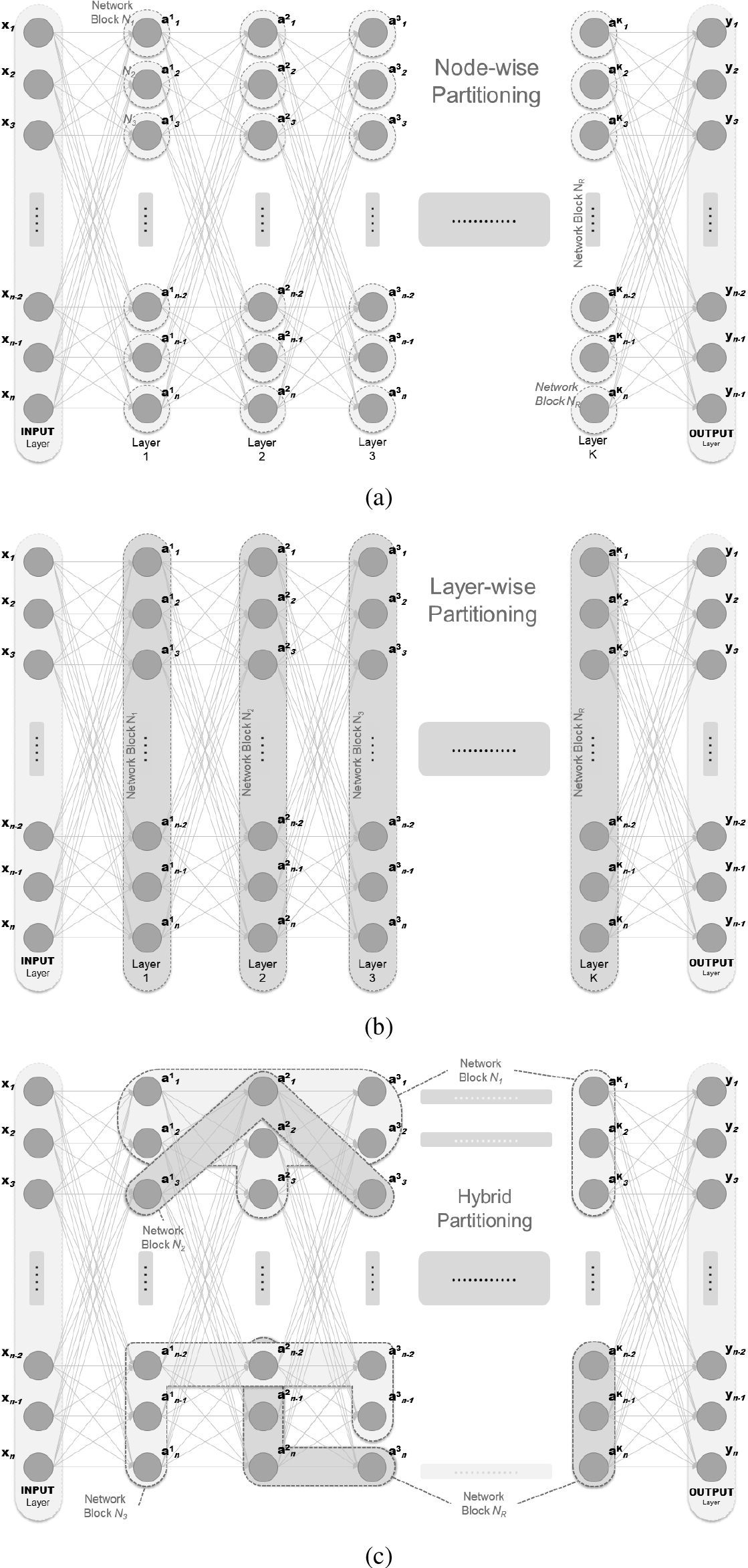
Splitting an Artificial Neural Network (ANN) into blocks or partitions can be done in different ways based on various factors such as network architecture, computational resources, and problem characteristics. To this end, the most common approach is to split the network by grouping layers into blocks (Layer-wise), or even into individual nodes or neurons (Node-wise). This approach can be useful when the computational resources are limited or when specific parts of the network require more parallelization. Each block would contain a subset of nodes and their corresponding connections would be limited to the nodes within the same block. Moreover dividing the network’s towards its parameters or weights into separate parts, each associated with a specific block or partition is another option (Parameter-wise). Such distribution may lead to improved scalability, reduced computational burden, and faster training times. However, the effectiveness of partitioning strategies depends on factors such as problem complexity, network architecture, and the communication and coordination mechanisms employed. Moreover, if the model performs multiple tasks or has multiple outputs, one may consider partitioning the network based on the tasks (Task-wise). Each block would focus on a specific task, allowing for independent training and optimization. Last but not least, a combination of the above approaches might be suitable. The model may be partitioned at multiple levels, such as layer-wise partitioning within each block and node-wise partitioning within certain layers. This can provide flexibility and customization based on the specific requirements of the problem. Based on Fig. 1 Neural Network, Fig. 2 Illustrates Node-wise, Layer-wise as well as Hybrid-wise partitioning. It should be mentioned that for simplicity reasons the number of nodes per layer has been considered the same and equal to n. The number of Layers is equal to K while the number of the partitioned Network Blocks (N1,N2,N3..NR) have considered equal with R. The ND-CAO algorithm is adequate to support every case of partitioning – in model parallel terms – since it is applicable to any potential splitting of ANN into blocks/partitions: Node-wise (n=R), Layer-Wise (K=R), Parameter-wise and potentially Task-wise and Hybrid-wise partitioning. To this end, the ND-CAO methodology significantly contributes to current gradient-free distributed algorithmic implementations, since current literature implementations are limited to Layer-wise Partitioning schemes – and that in solely synchronous training mode: current work exhibits Node-wise (Case I: FNN/MNSIT and Case II: FNN/Fashion MNIST) and Parameter-wise (Case III:CNN/MNIST and Case IV:CNN/CIFAR10) partitioning as indicative examples in order to reveal the adequacy of the algorithm to support such schemes.

All and all, the novelty attributes of the proposed algorithm may be summarized as follows:

• ND-CAO is applicable to any possible splitting of ANN into blocks/partitions.
• Each of the blocks is allowed to update its parameters fully asynchronously and independently of the rest of the blocks/partitions.
• Most importantly, no data exchange is required between the different blocks during training. The only information each block requires from “outside” is the global performance of the ANN.
• The training of each block is accomplished using a computationally inexpensive least-squares algorithm.
• Convergence of the ND-CAO is mathematically established for generic ANNs architectures, independently of the particular choices made for e.g., activation functions, etc. More precisely, it is shown that ND-CAO behaves approximately the same as asynchronous gradient-based BCD which was shown to converge to the same points as the ones of conventional fully centralized back propagation.

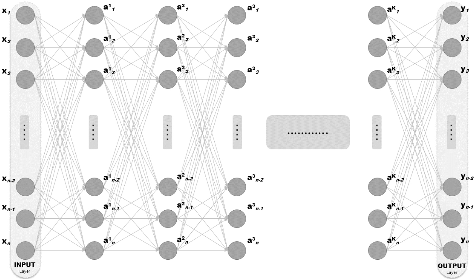
Figure 1.

Feed-forward ANN architecture.

ND-CAO aim represents the first approach that supports a distributed and also asynchronous training of Neural Networks. Except from illustrating a novel concept and mathematic methodology, this work illustrates also the adequacy of the algorithm for efficient distributed asynchronous training and indicates that such training scheme may be significantly beneficial in comparison to the conventional synchronous training scheme, using simulation results – at least as concerns the ND-CAO training scheme.

3.2Potential applications

Grounded on its unique novelty attributes ND-CAO training may prove a beneficial approach towards distributed model parallel training of large-scale models in image classification, natural language processing, financial forecasting applications, and more. However, ND-CAO scheme integrates a gradient-independent distributed and asynchronous training scheme, a unique attribute suitable to overcome the challenges of data exchange between geographically distributed models. Such particular frameworks require training each partition independently and updating its local model parameters based on local or global data or processing capabilities. It is envisaged that ND-CAO Asynchronous training is adequate to offer advantages in terms of scalability, privacy, and performance by reducing the reliance on continuous and synchronous data exchange between distributed locations. Such real-life frameworks may concern: a) Distributed IoT applications: where Neural networks are deployed on interconnected devices in various locations. ND-CAO asynchronous training enables efficient local model training without continuous data exchange between the sub-models; b) Multi-Cloud applications: Partitioned neural networks trained across diverse cloud environments across different geographical locations. ND-CAO asynchronous training allows independent updates limiting considering network latency and data transfer costs; c) Collaborative Research Applications: Multiple institutions contribute to a shared neural network model. ND-CAO Asynchronous training allows independent updates without constant real-time synchronization between the Network Blocks of the shared neural network; d) Federated Learning applications: Decentralized training on devices or servers in different locations. Local models are trained and aggregated to create a global model. ND-CAO distributed asynchronous updates may accommodate varying network conditions; e) Distributed Data Centers applications: Neural networks distributed across multiple data centers in different regions. ND-CAO Asynchronous training also independent updates considering network latency and limited bandwidth; f) Privacy-Preserving Learning applications: Data partitioned across geographic locations to ensure privacy. ND-CAO Asynchronous training enables local model updates without sharing raw data between different locations; g) Edge Computing applications: Neural networks on edge devices closer to a data source. ND-CAO asynchronous training is adequate to enable independent updates considering limited resources and intermittent connectivity.

Figure 2.

Examples of splitting an ANN into Neural Blocks (NBs). (a) Node-wise Partitioning: presents the partition of the NN that every NB corresponds to a node of the model; (b) Layer-wise Partitioning: presents the partition of the NN that every NB corresponds to a Layer of the model (K = R); (c) Hybrid-wise Partitioning: presents the partition of the NN partition the network at multiple levels.

4.The ND-CAO algorithm

4.1The set-up

We consider a quite standard ANN supervised learning setup. The ANN architecture is shown in Fig. 1 (for simplicity, we assume that the ANN has only feed-forward connections; the extension to the case where feedback connections are also present, is straightforward). Also, for simplicity the ANN shown in Fig. 1 is assumed to have equal number of nodes at each layer; the extension to the case of layers with different number of nodes is straightforward. The ANN of Fig. 1 has K hidden layers with N⁢(i) total neurons in the i-th layer; a⁢(i,j) denote the activation functions of the j-th neuron in the i-th layer; for convenience we assume that the 0-th layer is the input layer (with a⁢(0,j)≡xj, where xj denotes the j-th input; and (K+1)-th layer is the input layer (with a⁢(K+1,j)≡yj, where yj denotes the j-output. Let w=[w(1);w(2);…;w(K))] denote the synaptic matrix of the overall ANN of Fig. 1, with w(i) being the synaptic weights (including the biases) between layers i-1 and i. The output of the ANN satisfies

(1)

y=𝒩w⁢(x)

where 𝒩w⁢(⋅) is a nonlinear function that is parameterized by the weights w and depends on the number and width of the hidden layers and the activation functions of the neurons. As standard in most set-ups, we assume a set of N training data pairs (X,Y)=(x(s),y(s)),s=1,2⁢…,N. The problem at hand is to minimize of a cost function

ϵw⁢(X,Y)

with ϵw⁢(⋅) being a nonlinear function of its elements; the most “popular” choice for ϵw⁢(⋅) is ϵw⁢(X,Y)=1N⁢∑s=1N(y(s)-𝒩w⁢(x(s)))2. The proposed algorithm is applicable to any choice for the cost function ϵw⁢(⋅).

4.2ANN “break-down” into Neural Blocks (Asynchronous Agents)

Let us now assume that the overall ANN of Fig. 1 is “broken-down” into ℛ Neural1 1 Blocks (NBs) 𝒩1,𝒩2,…⁢𝒩ℛ satisfying the following:

• A synaptic weight wi⁢j(k) belongs only to one NB.
• There is no synaptic weight that does not belong to one of the NBs 𝒩1,𝒩2,…,𝒩ℛ.

The above two properties for splitting the ANN into ℛ NBs allow literally for any possible splitting of the ANN:

• from the extreme case where we have as many NBs as neurons, i.e., the case where each neuron is an NB, see e.g., Fig. 2(a);
• the case where each layer is an NB, see e.g., Figure 2(b);
• the cases where each NB consists of two or more layers;
• down to cases each NBs may be constructed by randomly picking synaptic weights across the ANN, see e.g., Fig. 2(c);
• and, many other configurations.

Given the above definition of NBs, let us define w(1),w(2),…,w(ℛ) be the synaptic weights of the 1st, 2nd, …,ℛ-th NB, respectively; apparently, [w(1);w(2);…;w(ℛ)≡w, i.e., the set of all synaptic weights of all NBs is equal to the set of all synaptic weights of the ANN of Fig. 1. Figure 2 exhibits different examples of splitting an ANN into NBs. Apparently, the most common partitioning schemes are the first two ones of Fig. 2 (node-wise and layer-wise partitioning). Also, in the case of geographically distributed ANNs, where parts of the ANN are located in different geographic locations, we may have a case where each of the NBs corresponds to one or more layers of the ANN. ND-CAO concept is quite generic that can handle all the aforementioned schemes of partitioning in a model parallel manner. Extreme cases – where e.g., a random partitioning is chosen – like the one of Fig. 2(c) can be also handled by our methodology.

4.3The learning algorithm

Consider each of the NB’s 𝒩1,𝒩2,…⁢𝒩ℛ and assume that the i-th NB 𝒩i is updating its synaptic weights every Δ⁢t(i) time-units. Note that Δ⁢t(i) may be different than some or all of the rest Δ⁢t(j),j≠i and that, also, Δ⁢t(i) is not necessary constant but may change at each updating cycle of the synaptic weights of the i-th NB 𝒩i. In other words, each of the NB’s updates its synaptic weights asynchronously as compared to the rest of NB’s and, thus, each of the NBs acts as an Asynchronous Agent – (AA). It is also worth noticing that the update frequency of each of the NBs does not have to be constant: our approach can facilitate non-constant (=non-periodic) updating.

The first key element of our approach is that each of the NBs is associated with an estimator which attempts – using only information available at the NB-level – to estimate the error (or, equivalently, the output) of the overall ANN.

More precisely, let k(i) denote the variable corresponding to the current number of updates of the synaptic weights of the i-th NB 𝒩i and let us associate to the i-th NB 𝒩i, the following Linear Local Estimator (LLE) of dimension L

(2)

ϵ^k(i)(i)=θk(i)(i)τ⁢ϕ(i)⁢(Zk(i)(i))

where ϵ^k(i)(i) denotes the output of the LLE associated with the ith NB, θk(i)(i) denote the L-dimensional vector of tune-able parameters of the LLE and ϕ(i) is a nonlinear L-dimensional vector function whose input Zk(i) is a vector comprising of (a) the synaptic weights wk(i)(i) of the i-th NB and (b) the measurements ϵw⁢(k(i)),ϵw⁢(k(i)-1),…,ϵw⁢(k(i)-d) of the cost function, where d is a positive integer (hyper-parameter). In other words,

Zk(i)(i)=[wk(i)(i)ϵw⁢(k(i))⋮ϵw⁢(k(i)-d)]

The purpose of the estimator (2) is to estimate the value of the global cost function ϵw⁢(X,Y) at the next update of the ith NB, using only local information available at the ith NB. In other words, by using information of a subset of the overall ANN inputs and synaptic weights, estimator (2) estimates and predicts the performance of the overall ANN. As we will see in the proof of Theorem 1, this possible thanks to the NDCAO special attributes.

For this reason, the choice of θk(i)(i) and ϕ(i) is made as follows:

• The vector θk(i)(i) of tune-able parameters is chosen – at the k(i)-t⁢h iteration of the learning algorithm – so as to minimize the error between the global cost function ϵw⁢(X,Y) and its estimation/prediction provided by the estimator (2):

(3)
θk(i)(i)=argmin𝜃⁢∑ℓ=k(i)-hk(i)-1(ϵw⁢(ℓ)-ϵ^ℓ(i))2

where h denotes a positive integer (size of time-window).
Problem (3) is a standard linear-least squares problem and can be solved using computationally inexpensive realizations of its least-squares solution:

(4)
θk(i)(i)=((Φk(i)(i))τ⁢Φk(i)(i))-1⁢(Φk(i)(i))τ⁢ℰk(i)

where Φk(i)(i)=[ϕ(i)⁢(Zk(i)(i)),…⁢ϕ(i)⁢(Zk(i)-h(i))] and ℰk(i)=[ϵw⁢(k(i)),…,ϵw⁢(k(i)-h)]τ.
As it was shown in [92], it is sufficient for learning algorithms like NDCAO that employ estimators of the form (2), to approximate locally the global cost function. As this global cost function is a quadratic one, it is sufficient to use linear and second-order terms for its local approximation. For this reason, the nonlinear vector function comprises L first and second-order polynomial terms; typically, these L terms are randomly chosen among all possible first and second-order polynomial terms.

The second key element in our approach is to employ – at its NB level and totally asynchronously with respect to the rest of the NBs – the estimator (2) to test different perturbations of the current value of the synaptic weights and pick the one that produces the “best” estimate/prediction for the global cost function. The overall methodology combining the two key elements of the methodology is summarized in Algorithm 1.

We proceed with the convergence analysis of the algorithm. We have the following theorem.

Theorem 1. At each time-instant k, the ND-CAO algorithm satisfies

wk(i)+1(i)=wk(i)(i)+αk(i)⁢∇w(i)|w=wk(i)⁢ϵw⁢(X,Y)+𝒪⁢(ak(i)/L)

Remark 1. In simple words, Theorem 4.3 establishes that the ND-CAO algorithm behaves similarly to asynchronous gradient-based BCD “disturbed” by the term 𝒪⁢(ak(i)/L) which vanishes as time increases. □

Remark 2. As it has been established in many different papers – see e.g. [93] and the references therein – asynchronous gradient-based BCD converges to the same points as the ones of conventional fully-centralized backpropagation. Therefore, Theorem 4.3 establishes convergence of the ND-CAO algorithm the same points as the ones of conventional fully-centralized back propagation:

Algorithm 1: Asynchronous ND-CAO Algorithm
Definitions/Initializations:
• Let the ANN being split into ℛ NBs (Neural blocks). Also, for simplicity let us assume that each of the LLEs of the ℛ NBs has dimension L. • Let also each NB update its parameters asynchronously; let Δ⁢t(i) denote the time-units the i-th NB 𝒩i is updating its synaptic weights, with Δ⁢t(i) being not necessarily constant. • Let k(i) be a current number of updates of the synaptic weights of the i-th NB 𝒩i. • Let also αk(i) be a user-defined positive scalar sequence satisfying limk(i)↦∞⁡αk(i)=0,∑k(i)=0∞αk(i)=∞,∑k(i)=0∞αk(i)<∞ and K(i) be a user-defined constant integer satisfying K(i)⩾2⁢dim⁡(wk(i)(i)). fori=1:ℛdo
1. Step 1 – Estimate locally the Global Cost Function. Generate estimate ϵ^k(i)(i) using (2). 2. Step 2 – Find the “Best” Candidate Perturbation. Generate a set of K(i) random (or pseudo-random) zero-mean candidate perturbations (5) δ1(i)⁢(k(i)),δ2(i)⁢(k(i)),…,δK(i)(i)⁢(k(i)) Find the candidate perturbation δj(i)⁢(k(i)) of the current synaptic weight vector wk(i)(i) that will have the “best effect” to the estimated cost function (6) δj(i)⁢(k(i))=argminj=1,…,K(i)⁢(θk(i)(i)τ⁢ϕ(i)⁢(Zj,k(i)(i))) where Zj,k(i)(i)=[(wk(i)(i)+αk(i)⁢δj(i)⁢(k(i)))ϵw⁢(k(i))⋮ϵw⁢(k(i)-d)] 3. Step 3 – Update NB synaptic weights. Update wk(i)(i) according to (7) wk(i)+1(i)=wk(i)(i)+αk(i)⁢δj(i)⁢(k(i)) 4. Step 4 – Update parameters of the estimator (2).* Update the parameters θk(i)(i) of the estimator (2), using (4).
= 0

• for any possible splitting of ANN into Neural Blocks (NBs), including even blocks elements may be totally disconnected;
• with each of the NBs allowed to update their parameters fully asynchronously and independently of the rest of the NBs;
• no data exchange is required between the different blocks during training with the only information each block requires from “outside” is the global performance of the ANN;
• The training of each NB is accomplished using a computationally inexpensive least-squares algorithm. □

< Numbering of Theorem corrected to Theorem 1 (“Theorem 2.3” was a typo) >

Proof of Theorem 1: A brief outline of the proof is given, as its derivation closely mirrors the proof process of Theorem 2 of [57], by simply performing the following “time-transformation”: consider a sufficiently small Δ⁢t such that the weights of each of the NBs are updated always at some time-instances t(i) that satisfy t(i)=n⁢Δ⁢t for some integer n. Then, Theorem 2 of [57] holds for the case of the asynchronous ND-CAO by assuming that w(i) is updated at time-instances t(i)=n⁢Δ⁢t and remains constant at all other time-instances. Using this transformation and following the same arguments as the ones in the proof of Theorem 2 of [57], we have that

ϵwk(i)⁢(X,Y)=E⁢(wk(i)(i),ϵwk(i)-1⁢(X,Y),…,ϵwk(i)-d⁢(X,Y))

for some nonlinear function E⁢(⋅), i.e., the cost function ϵw⁢(X,Y) – which depends on the whole weight vector w – can be also written as a function E⁢(⋅) which depends on the “local” sub-vector w(i) of the ith NB as well as of past measurements of the cost function ϵw⁢(X,Y). On the other hand, following the same steps as in [92], it can be seen that Eqs (5)–(7) are equivalent to

wk(i)+1(i)=wk(i)(i)+αk(i)⁢∇w(i)|w=wk(i)⁢E⁢(wk(i)(i),ϵwk(i)-1⁢(X,Y),…,ϵwk(i)-d⁢(X,Y))+𝒪⁢(ak(i)/L)

Combining the two above equations, we establish the proof. □

5.Experimental evaluation of ND-CAO asynchronous training

Table 1

Use case description and setup features

Case	Dataset	Input shape	Model type	Model architecture	Weights	Partitioning scheme	Asynchronous agents	Epochs
I	MNIST	28 × 28 × 1	FNN	32 × 10	320	Node-wise: 1 Agent/Node	0, 10, 20, 30, 40	5000
II	Fashion MNIST	28 × 28 × 1	FNN	32 × 16 × 10	672	Parameter-wise: 1 Agent/Node	0, 10, 20, 30, 40, 50, 55	1000
III	MNIST	28 × 28 × 1	CNN	32 × 32 × 10	25258	Parameter-wise: 1 Agent/1000 Weights	0, 10, 20, 30, 40	2500
IV	CIFAR10	32 × 32 × 3	CNN	32 × 32 × 10	25258	Parameter-wise: 1 Agent/1000 Weights	0, 10, 20, 30, 40	2500

In this section, we examine ND-CAO adequacy in training neural networks of different architectures, towards image classification problems, giving also emphasis on asynchronous mode training. Asynchronous training can provide several benefits over synchronous training, especially towards a distributed model. For example, it can improve the speed of training as the blocks can update the model weights independently and in parallel. Additionally, it can handle scenarios where the blocks need different computing capabilities or network bandwidth, as each block can work at its own pace without waiting. Before proceeding to the detailed description of the four experimental Cases and their integrated simulations, it is appropriate to describe some initial conditions and frameworks that served equally the procedures in order to implement the experiments. Table 1 describes at a high level the four experimental Cases:

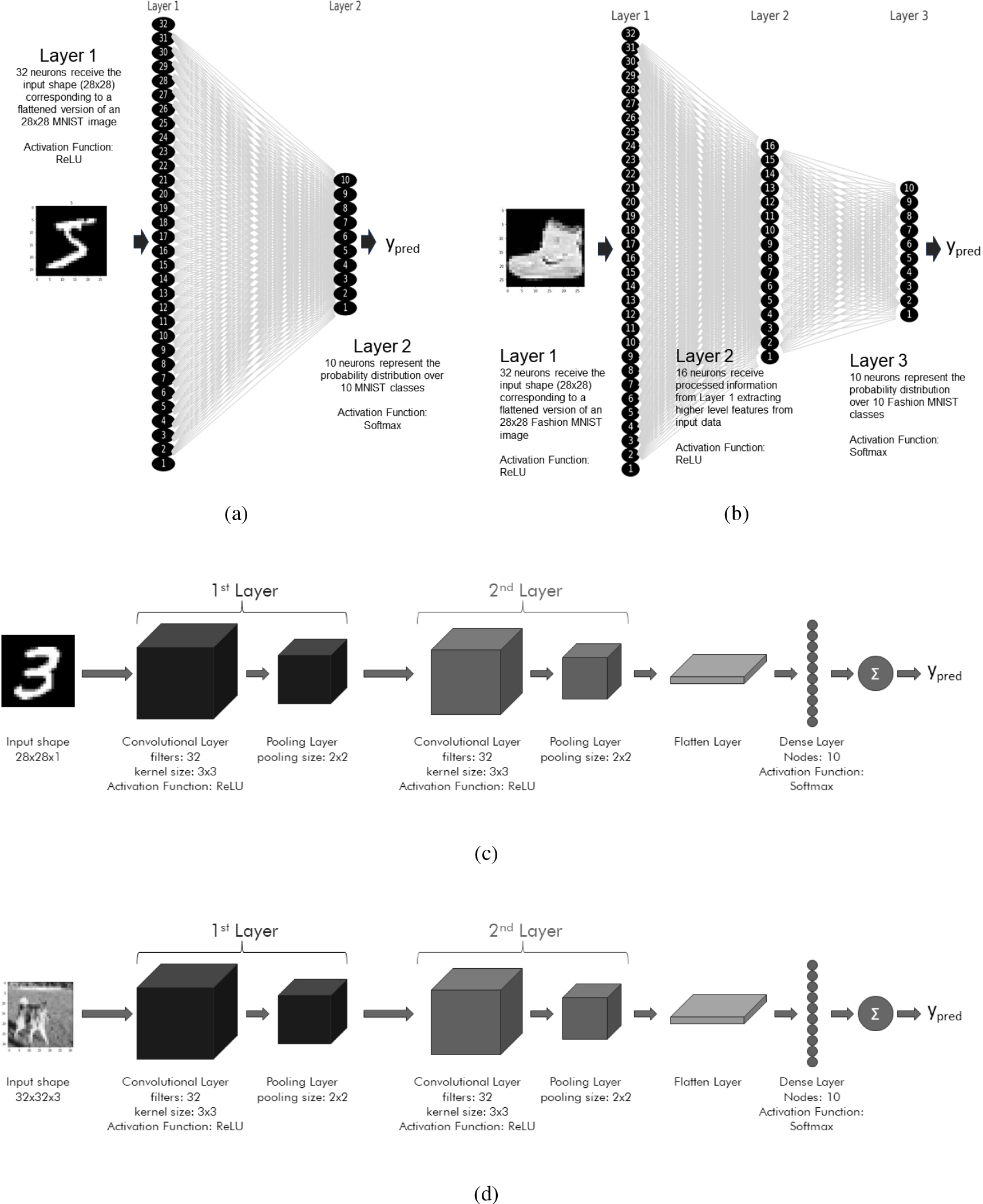
Datasets, model type, architecture, and number of training epochs: Case I concerns an FNN model for addressing the MNIST image classification problem in 5000 epochs, Case II concerns a more demanding FNN model for addressing the Fashion MNIST image classification problem in 1000 epochs, Case III concerns a CNN model for addressing the MNIST image classification problem in 2500 epochs, and Case IV concerns a CNN model for addressing the CIFAR10 image classification problem in 2500 epochs. In Fig. 3 the (a), (b), (c) and (d) subfigures, illustrate the architecture of Case I, Case II, Case III, and Case IV models respectively.

Asynchronous agents: Additionally. we have considered the same following asynchronous training scenarios: at each time instant, N randomly chosen NBs are not updated their parameters while the rest 42 N Network Blocks (NBs) or Asynchronous Agents (AA) are updated using ND-CAO. In ND-CAO asynchronous training mode, each partition updates its parameters independently, without the need to wait for updates from other partitions; To this end, five different scenarios for N= 0 (synchronous case-baseline), N=10, N=20, N=30, N=40 were executed and through their evaluation and comparison, fruitful conclusions arise. Moreover as concerns the distribution scheme that has been adopted

Partitioning scheme: It should be also underlined that in Case I and Case II, the Network Blocks (NBs) have been elected to act as Asynchronous Agents/Nodes (AA) in order to implement a Node-wise Partitioning scheme while in Case III and Case IV, the agents of ND-CAO concern a certain amount of parameters (1000 weights per agent – 42 agents overall) in order to implement a more sophisticated Parameter-wise partitioning scheme. Last but not least, It should be mentioned, that in our work the selection of the asynchronous agents per epoch is taking place in a random manner in order to exhibit the adequacy of our approach to training the networks under totally stochastic conditions. The primary conclusions of the comparison between ND-CAO synchronous and ND-CAO asynchronous training exhibit the adequacy and efficiency of the algorithm.

Hardware and software: As regards the hardware and software equipment it acted equally for all four Cases (4 × 5 overall simulations):

• Hardware: The computational machine that all experiments took place considered a conventional x64 – based PC setup holding the following characteristics CPU: AMD Ryzen 7 5800X / 8 cores, 3801 Mhz; GPU: NVIDIA GeForce RTX 3060 Ti / 8 GB; RAM: Corsair Vengeance RGB Pro / 32GB;
• Software: The concerned PC was operating Windows 11 Pro. Python 3.8 Code Framework was enabled and acted as the ground for constructing the algorithm and executing all four experimental simulations for ND-CAO evaluation. The Primary Python Machine Learning Libraries that were utilized concerned: numpy, scipy, multiprocessing (mp) module, keras, scikit-learn, pandas and openpyexcel.

Figure 3.

Detailed architecture of the examined Neural Network cases: (a) Case I: Feed-forward NN over MNIST; (b) Case II: Feed-forward NN over Fashion MNIST; (c) Case III: Convolutional NN over MNIST, and (d) Case IV: Convolutional NN over CIFAR10.

The following subsections of the paper describe the Setup of each experimental Case in detail, providing the dataset information, the deployed network architecture, the elected distribution scheme that took place, and the settings of the five experimental scenarios for each Case. Next, after illustrating the training results in Figs 4, 5, and Fig. 6 for Case I, Case II, Case III, and Case IV respectively, a brief Evaluation is conducted for every respective case. The last subsection of the Results Section concerns the final Verdict where fruitful conclusive notes are drawn, considering the training of ND-CAO efficiency in synchronous and asynchronous modes.

5.1Case I: ND-CAO asynchronous training evaluation on FNN – MNIST

The first set of experiments took place, concerning a typical Feedforward ANN of 42 NBs being trained over the MNIST dataset in synchronous and asynchronous modes. The summary of the Use case Description setup may be found under Table 1 – Case I.

5.1.1Setup – Case I

Dataset information: It should be mentioned that the MNIST dataset contains a total of 70,000 data items. These items are split into two main subsets: a training set and a test set. The training set consists of 60,000 handwritten digits from 0 to 9, while the test set contains 10,000 handwritten digits. Each data item in the MNIST dataset represents a 28 × 28 grayscale image of a handwritten digit, making it a widely used benchmark dataset for machine learning tasks, especially in the field of image classification.

Neural Network Architecture: In this case, each NB (Network Block) or ND-CAO agent considers a single ANN neuron. The ANN architecture consists of two dense (fully connected) layers: The first layer is a dense layer with 32 neurons, using the ReLU activation function. This layer takes the input of shape (28 × 28), which corresponds to a flattened version of a 28 × 28 image. The second layer is a dense layer with 10 neurons, using the softmax activation function. This layer outputs a probability distribution over 10 classes, which can be interpreted as the model’s prediction for the input image. The model is then compiled using the Adam optimizer, categorical cross-entropy loss function, and categorical accuracy as the evaluation metric. Overall, this architecture portrays a simple Feed-Forward neural network (FNN) suitable for image classification tasks on small datasets. The full Architecture of the FNN is illustrated in Fig. 3(a).

Distribution type and features: This initial scenario concerns a Node-wise Partitioning scheme since Network Blocks (NBs)/Asynchronous ND-CAO Agents (AA) have been elected to act as Asynchronous Nodes. The choice N=0 corresponds to the fully synchronous training case.

Experimental scenarios: We have considered the following asynchronous training scenarios, at each time instant, where N randomly chosen NBs are not being updated while the rest 42-N NBs are being updated using ND-CAO. 5 different choices for the integer N were tested, N=0, N=10, N=20, N=30, N=40. Training Epochs have been set to 5000 for each scenario of the 5 experimental simulations.

5.1.2Evaluation – Case I

Figure 4.

Asynchronous ND-CAO for training FNN towards MNIST: (a) Loss per Epoch, (b) Accuracy per Epoch.

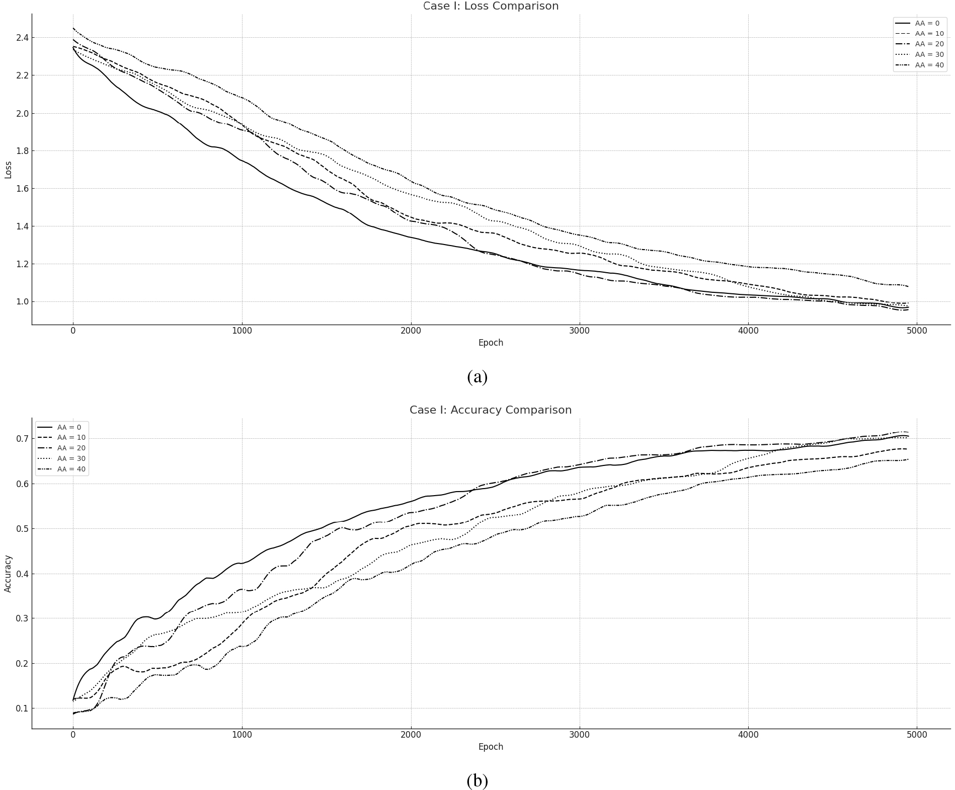
The results overall are presented in Loss and Accuracy measures in Fig. 4: (a) presents the overall Loss during training while (b) Illustrates the Accuracy of the Network. The course of all the training simulations is potentially the same and convergence is guaranteed for each case scenario. The Asynchronous cases (N=10 – Red Line, N=20 – Orange Line, N=30 – Pink Line, N=40 – Green Line) follow the Synchronous training (N=0 – Blue Line) tendency in every epoch as concerns Loss and Accuracy measures. It is noticeable that for a certain time of epochs (epoch 2500), the N=20 Asynchronous case surpasses the N=0 synchronous case in Loss and Accuracy measures (2500 epoch). Moreover, after 5000 epochs of training N=0, N=10, N=20, N=30 synchronous and asynchronous simulation cases converge to almost the same Loss and Accuracy measures while the N=40 asynchronous case performance is slightly decreased.

5.2Case II: ND-CAO asynchronous training evaluation on FNN – Fashion MNIST

The second set of experiments took place, concerning a similar Feedforward NN being trained over the Fashion MNIST dataset in synchronous and asynchronous modes under 1000 Epochs. While the implementation concerns similarly a Node-wise partitioning to Case I, the FNN architecture is more deep and serves a relatively more demanding image classification task by utilizing 58 ND-CAO agents. The primary aim of this implementation is to illustrate the adequacy of ND-CAO training in synchronous and asynchronous modes over a potentially more complicated network, under a more demanding dataset. The summary of the Use case Description setup may be found under Table – Case II.

5.2.1Setup – Case II

Dataset information: Fashion MNIST is a dataset commonly used for image classification tasks. It consists of 60,000 grayscale images of 10 different clothing categories, with each image having a size of 28 × 28 pixels. The dataset is a drop-in replacement for the original MNIST dataset and serves as a more challenging benchmark for evaluating machine learning models. It provides a realistic representation of real-world image classification problems and allows researchers to compare the performance of different algorithms on a more diverse set of images. Fashion MNIST has become popular in the deep learning community as a standard dataset for testing and developing new models and algorithms.

Neural network architecture: Similarly to Case I, each NB (Network Block) or ND-CAO agent considers a single NN neuron. The NN architecture consists of three dense (fully connected) layers: The first hidden layer is a dense layer with 32 neurons, using the ReLU activation function. This layer takes the input of shape (28 × 28), which corresponds to a flattened version of a 28 × 28 image. The second hidden layer is a dense layer with 16 neurons utilizing also ReLU activation function. The third output layer consists of 10 neurons, using the softmax activation function. This layer outputs a probability distribution over 10 classes, which can be interpreted as the model’s prediction for the input image. The full Architecture of the FNN is illustrated in Fig. 3(b). In summary, the 32 × 16 × 10 FNN provides a deeper and more expressive architecture compared to the 32 × 10 FNN, allowing for potentially better representation and learning of complex features in the Fashion MNIST dataset. However, the increased complexity comes with the cost of additional parameters to train and potentially longer training times.

Distribution type and features: Case II concerns a relatively more demanding Node-wise Partitioning scheme considering 58 nodes overall being updated by 58 Asynchronous ND-CAO Agents (AA). The choice N=0 corresponds to the fully synchronous training case.

Experimental scenarios: Similarly the training scenarios have considered the same number of asynchronous agents and one additional of 50 AA (Tirquise line): at each time instant, N randomly chosen NBs are not being updated while the rest 58-N NBs are being updated using ND-CAO. 5 different choices for the integer N were tested, N=0, N=10, N=20, N=30, N=40, N=50. Training Epochs have been limited to 1000 for each scenario of the 5 experimental simulations.

5.2.2Evaluation – Case II

Figure 5.

Asynchronous ND-CAO for training CNN towards MNIST: (a) Loss per Epoch, (b) Accuracy per Epoch.

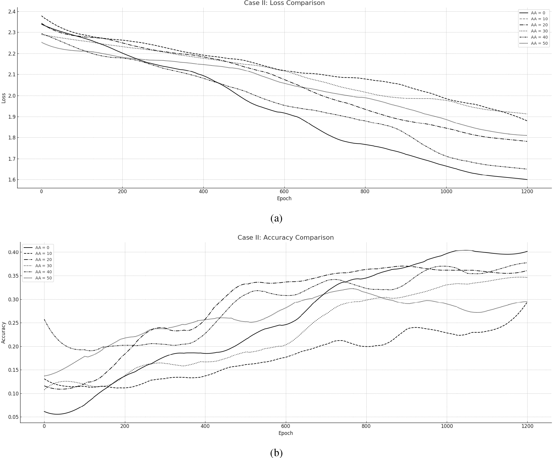
This particular experiment was executed for 1000 epochs revealing also the efficiency of ND-CAO in both synchronous and Asynchronous manner in Fig. 5. Scenario N=0 (blue line) was more efficient for 1000 Epochs while the rest revealed the same tendency. N=40 scenario (green line) portrayed the most fruitful scenario of all the asynchronous cases following closely the N=0 synchronous scenario. The rest of the cases N=10, N=20, N=30, N=50 exhibited significantly less performance in Loss and Accuracy measures than the above-mentioned N=0 and N=40 towards the particular limited Epoch range (1000 Epochs).

5.3Case II: ND-CAO asynchronous training evaluation on FNN – Fashion MNIST

The third set of experiments took place, concerning a Convolutional Neural Network (CNN) (32 × 32 × 10) being trained over MNIST dataset in synchronous and asynchronous scenarios. Each ND-CAO Network block is set to 1000 weights. The summary of the Case III Use case description setup may be found under Table 1 – Case III.

5.3.1Setup – Case III

Dataset information: The dataset information of MNIST has already give in Case I. However, the architecture and design principles of a CNN portray a potentially well-suited model for image classification tasks like MNIST, allowing to capture spatial information, exploit parameter sharing, handle translation invariance, and learn hierarchical representations, resulting in improved prediction performance.

Neural network architecture: The model portrays a convolutional neural network (CNN) designed for image classification tasks taking as input grayscale images of MNIST (size 28 × 28 pixels). Overall, this model architecture consists of two sets of convolutional and max pooling layers for feature extraction, followed by a flatten layer to convert the output into a 1D vector. Finally, a dense layer with softmax activation is used for class probability predictions. The overall weights of the CNN reach 25258. he model is compiled with the following settings: Optimizer: Adam, Loss function: Categorical cross-entropy, Evaluation metric: Categorical accuracy. More specifically

• Convolutional Layer 1: Number of filters: 32, Kernel size: 3 × 3, Activation function: ReLU)
• Max Pooling Layer 1: Pooling size: 2 × 2
• Convolutional Layer 2: Number of filters: 32 (Kernel size: 3 × 3, Activation function: ReLU)
• Max Pooling Layer 2: Pooling size: 2 × 2
• Flatten Layer: Converts the output from the previous layer into a 1D vector for input to the dense layers
• Dense Layer: The number of neurons is 10, producing a probability distribution over the 10 possible classes (Activation function: Softmax)

The full Architecture of the FNN is illustrated in Fig. 3(b).

Distribution type and features: In this distribution scheme we have elected to dedicate one ND-CAO agent towards 1000 weights of the neural network. Such Parameter-wise partitioning involves dividing the network’s parameters or weights into separate parts, each associated with a specific block or partition. This partitioning allows different parts of the network to be trained or updated independently while still working towards the common goal of minimizing the overall error.

Experimental scenarios: Similarly to Case I, we have considered the following asynchronous training scenarios, at each time instant, N randomly chosen NBs are not updated while the rest NBs weigh are updated their parameters using ND-CAO. Five different choices for the integer N were evaluated, N=0, N=10, N=20, N=30, N=40. Training Epochs have been set to 2500 for each of the five experimental simulations.

5.3.2Evaluation – Case III

The results overall are presented in Loss and Accuracy measures in Fig. 6: (a) presents the overall Loss during training while (b) Illustrates the Accuracy of the Network. The course of all the training simulations is potentially the same and convergence is guaranteed for each case scenario. The Asynchronous cases (N=10 – Red Line, N=20 – Orange Line, N=30 – pink Line, N=40 – Green Line) follow the Synchronous training (N=0 – Blue Line) tendency in every epoch as concerns Loss and Accuracy measures. In this set of scenarios, the synchronous case (N=0 – blue line) outperforms all asynchronous cases.

Figure 6.

Asynchronous ND-CAO for training CNN towards MNIST: (a) Loss per Epoch, (b) Accuracy per Epoch.

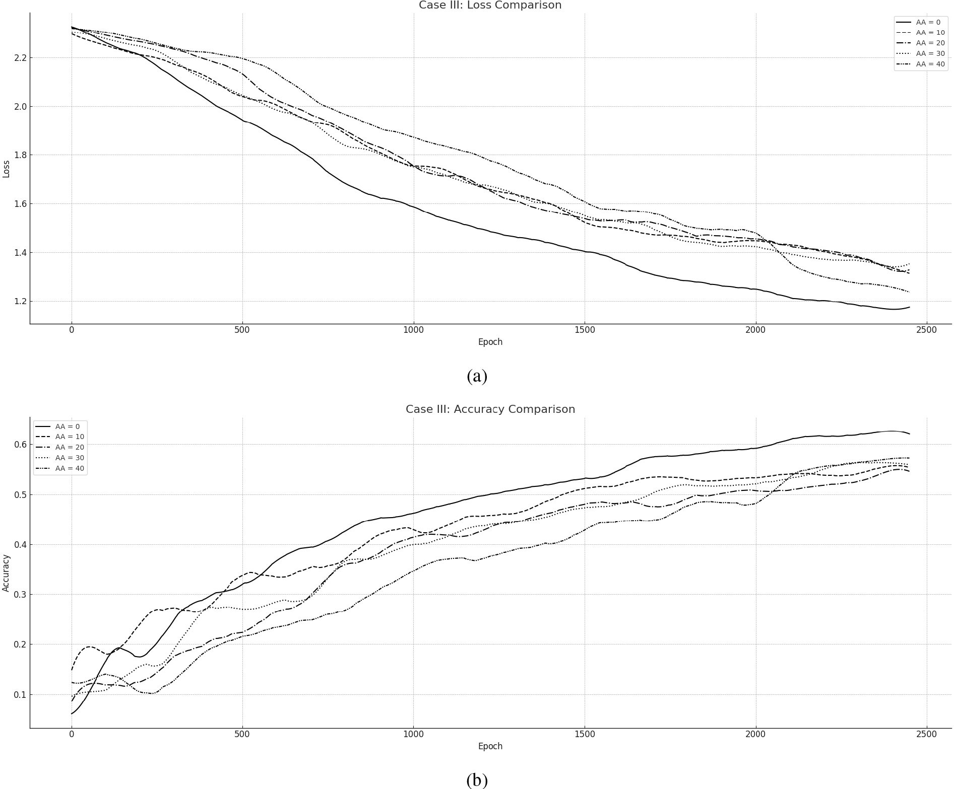
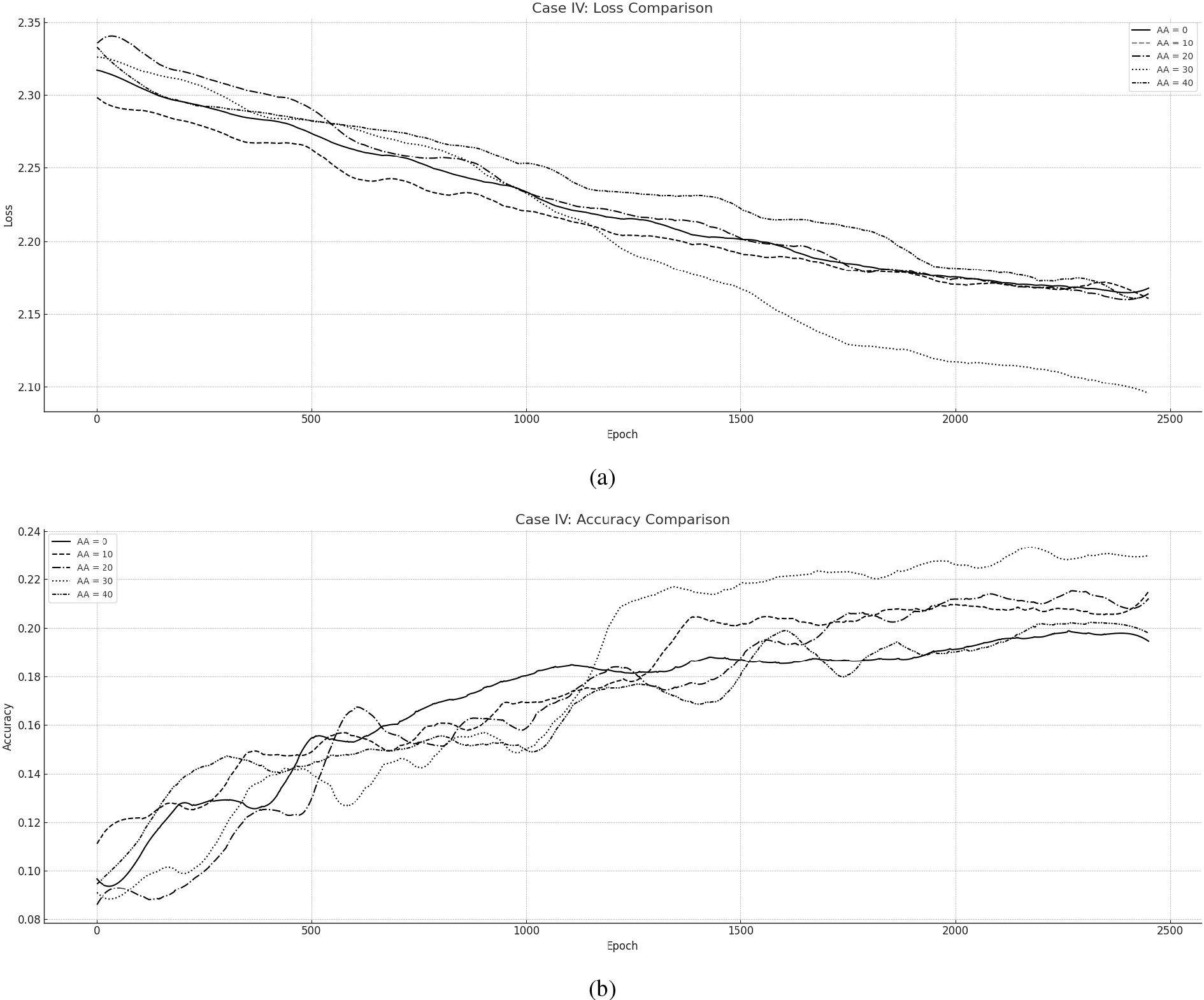
However, the asynchronous cases – and especially the N=40 asynchronous scenario that tends to converge closer at 2500 epoch – potentially required less training time as well as less computational and communicational demand overall. It is noticeable that for a certain period of 2500 epochs, the most advantageous asynchronous case is the N=40 setting (green line) Fig. 6 which is converging closely to the synchronous case after 2000 epochs at least in loss measure.

5.4Case IV: ND-CAO asynchronous training evaluation on CNN – CIFAR10

The fourth set of experiments took place, concerning the same Convolutional Neural Network (CNN) being trained over the more challenging CIFAR10 dataset, in synchronous and asynchronous scenarios. The summary of the second Use case description setup may be found under Table – Case IV.

Figure 7.

Asynchronous ND-CAO for training CNN towards CIFAR10: (a) Loss per Epoch, (b) Accuracy per Epoch.

5.4.1Setup – Case IV

Dataset information: The CIFAR10 represents a widely used benchmark dataset in the field of computer vision and machine learning. It consists of 60,000 32 × 32 color RGB images (32 × 32 × 3) in 10 different classes, with 6,000 images per class (Airplane, Automobile, Bird, Cat, Deer, Dog, Frog, Horse, Ship, Truck). The dataset is divided into two subsets, a training set, and a test set. The training set contains 50,000 images, with an equal number of images from each class while The test set contains 10,000 images, also evenly distributed across the 10 classes.

Neural network architecture: The CNN model portrays a convolutional neural network (CNN) designed for image classification tasks taking as input RGB images of CIFAR10 (size 32 × 32 pixels). Overall, this model architecture is similar to Case III and has compiled with identical settings: Optimizer: Adam, Loss function: Categorical cross-entropy, Evaluation metric: Categorical accuracy. More specifically:

• Convolutional Layer 1: Number of filters: 32, Kernel size: 3 × 3, Activation function: ReLU)
• Max Pooling Layer 1: Pooling size: 2 × 2
• Convolutional Layer 2: Number of filters: 32 (Kernel size: 3 × 3, Activation function: ReLU)
• Max Pooling Layer 2: Pooling size: 2 × 2
• Flatten Layer: Converts the output from the previous layer into a 1D vector for input to the dense layers
• Dense Layer: The number of neurons is 10, producing a probability distribution over the 10 possible classes (Activation function: Softmax)

The full Architecture of the CNN is illustrated in Fig. 3(d).

Distribution type and features: Similarly to Case III, the distribution scheme considers Parameter-wise partitioning where one ND-CAO agent updates 1000 weights of the model. This partitioning allows different parts of the network to be trained or updated independently while still working towards the common goal of minimizing the overall error.

Experimental scenarios: Similarly to Case I and Case III, Case IV integrates a set of five simulations which have been implemented considering the following asynchronous training scenarios, at each time instant, N randomly chosen NBs are not updated while the rest NBs are updated using ND-CAO agents; similarly, five different choices for the integer N were evaluated, N=0, N=10, N=20, N=30, N=40. Training Epochs have been set also to 2500 for each of the five simulation scenarios.

5.4.2Evaluation – Case IV

The results overall are presented in Loss and Accuracy measures in Fig. 7: (a) presents the overall Loss during training while (b) Illustrates the Accuracy of the Network. The course of all the training simulations is perfectly identical however, convergence is guaranteed for each case scenario. The Asynchronous cases (N=10 – Red Line, N=20 – Orange Line, N=40 – Green Line) achieve slightly better performance than the Synchronous baseline training scenario (N=0 – Blue Line). The asynchronous scenario of N=30 however (N=30 – pink Line), substantially surpasses every other synchronous or asynchronous scenario in Loss and Accuracy measures between 1000–2500 epochs.

To this end, and similarly to Case I Case II, and Case III, Case IV asynchronous scenarios converge towards the synchronous case as Fig. 7 illustrates. However, the synchronous case does not portray the best potential training setting, since the N=30 scenario surpasses significantly the N=0 synchronous scenario in Loss and Accuracy measures while potentially concerning less computational, communicational, and training time demand at 2500 epochs.

5.5Verdict

The primary verdict of the Evaluated comparison between ND-CAO synchronous and ND-CAO asynchronous training arising from Figs 4, 5, 6 and 7 exhibits the adequacy of the algorithm to training neural networks in a gradient-free and distributed manner in both synchronous and asynchronous modes under different model architectures. The primary attributes of ND-CAO evaluation may be summarized as follows:

• Note 1 – ND-CAO training efficiency: One important attribute observed in all of the synchronous and asynchronous training cases is that ND-CAO achieved both Loss and Accuracy convergence close to the Synchronous ND-CAO reference case: by the examination of two FNNs and two CNNs case scenarios concerning different image classification problems (MNIST, Fashion MNIST, CIFAR10), ND-CAO exhibited its robustness and efficiency for training in both synchronous and asynchronous modes in an adequate manner.
• Note 2 – ND-CAO Asynchronous training capability: ND-CAO was operational even in cases where a substantial number of neurons or parameters were potentially deactivated (e.g. the scenarios of N=40 in Case I, Case II, Case III, and Case IV portrayed by a green line). Such an attribute, indicates the operational efficiency of the algorithm in cases of asynchronous learning, even when a significant number of nodes, partitions, or parameters of the model are potentially deactivated for different reasons or purposes. It is also noticeable that in Case II and Case III, the N=40 setting outperforms all other asynchronous scenarios, while in Case IV the N=30 scenario turned to achieve significant improvements in Loss and Accuracy measures in comparison to synchronous and asynchronous scenarios in 2500 epochs. In other words, it is potentially beneficial to deploy ND-CAO asynchronous scenario over a synchronous one since performance will be similar, while training time and computational demand will be significantly decreased.
• Note 3 – Parameters Optimization requirement: It is noticeable that there is a critical number of deactivated nodes that results in the best possible outcome of each potential model. That number is potentially different for every model and is being affected by diverse parameters that are resulting in the best possible outcome in Loss and Accuracy measures: model architecture, training epochs, dataset characteristics, etc. To this end, before deploying an asynchronous training mode, it is beneficial to determine the potential features that suit the model and its potential characteristics. Such type of optimization is not an easy task, however, and thus, it paves the way for more essential research work that may be generated in the future.
• Note 4 – ND-CAO distribution adequacy: Last but not least, ND-CAO achieved to adequately respond to synchronous or asynchronous training challenges towards different distribution schemes. While Case I and Case II concerned a Node-wise distributing scheme, Case III and Case IV which preserved a significantly larger number of parameters, considered a more sophisticated Parameter-wise distributing scheme. Such attribute indicates the novelty of the algorithm to support gradient-free distributed training of ANNs in a wide range of applications that demand multifunctional distribution schemes e.g. Task-wise or Hybrid-wise partitioning schemes that have never been illustrated in the literature as concern gradient-free distributed methodologies.

6.Conclusions and future work

ND-CAO methodology, portrays a novel gradient-free and distributed algorithmic scheme, capable to support synchronous and asynchronous training. Grounded on its conceptual background, the algorithm proved adequate to support any potential partitioning scheme – in a model parallel manner and eliminate the data exchange between the network blocks during training. Contrary to conventional approaches, ND-CAO proved sufficient to update the parameters of each network block fully independently and asynchronously, towards global error minimization: ND-CAO proved adequate to train each scenario efficiently without requiring a definition of discrimination areas – in local areas – for a given network configuration. Moreover, interesting results have arisen from the comparison between the synchronous training – which acted as the baseline – and the asynchronous settings in each case scenario. As the comparison indicates for Case I, Case II, Case III, and Case IV, ND-CAO asynchronous approach proved quite beneficial in numerous scenarios evaluations – in terms of Loss and Accuracy measures over a certain number of epochs. Taking in mind that asynchronous training is additionally advantageous in training time, computational, and communicational demand, such benefits are extended even further.

Such properties deliver a quite optimistic perspective for the future utilization of the algorithm and potentially contribute to the challenging training of large-scale neural networks that require gradient-free distributed and asynchronous training that is prohibited by the limitations of conventional approaches. It should be mentioned that this work portrays the first literature work that a gradient-free distributed algorithmic framework has been successfully utilized for asynchronous training – in a model parallel terms and thus, it paves the way for addressing challenging distributed deep learning problems that haven’t been satisfied – or have merely satisfied. Moreover, the current work portrays the first gradient-free and distributed scheme that is being evaluated for Node-wise and Parameter-wise partitioning, since the literature integrates applications that have solely concerned Layer-wise partitioning applications.

Future work is already planned to investigate the behavior of ND-CAO in broader contexts, such as the utilization of the algorithm towards challenging asynchronous training of neural networks regarding the Internet of Things (IoT), Multi-Cloud Environments, Federated Learning, Distributed Data Centers, Privacy-Preserving Learning, Collaborative Research and more where challenges of data exchange between geographically distributed partitions limiting the application potential of conventional methodologies. Future work will additionally focus on newer supervised machine learning/classification algorithms as part of a potential extension of ND-CAO, such as Neural Dynamic Classification algorithm, Dynamic Ensemble Learning Algorithm, Finite Element Machine for fast learning, and self-supervised learning [94, 95, 96]. More specifically, ND-CAO asynchronous methodology performance is expected to be enhanced, by adopting different policies for selectively updating partitions of the NN in order to further upgrade its efficiency. Additionally, ND-CAO is planned to act as a training framework for asynchronous learning on large-scale NNs and be compared with the already evaluated gradient-based asynchronous approaches. Last but not least, the novel algorithm is planned to generate a hybrid framework between ND-CAO and gradient-based methodologies, in order to embrace both advantages and create a fruitful ecosystem of algorithmic CAO-based tools, targeting to address specific challenging machine learning problems.

Notes

1 Throughout this paper, the terms “Neural Blocks (NBs)” and “Asynchronous Agents (AAs)” is used interchangeably.

Acknowledgments

We acknowledge support of this work by the project “Study, Design, Development and Implementation of a Holistic System for Upgrading the Quality of Life and Activity of the Elderly” (MIS 5047294) which is implemented under the Action “Support for Regional Excellence”, funded by the Operational Programme “Competitiveness, Entrepreneurship and Innovation” (NSRF 2014-2020) and co-financed by Greece and the European Union (European Regional Development Fund).

References

[1]	Liapis S, Christantonis K, Chazan-Pantzalis V, Manos A, Elizabeth Filippidou D, Tjortjis C. A methodology using classification for traffic prediction: Featuring the impact of COVID-19. Integrated Computer-Aided Engineering. (2021) ; 28: (4): 417-35.
[2]	Islam S, Abba A, Ismail U, Mouratidis H, Papastergiou S. Vulnerability prediction for secure healthcare supply chain service delivery. Integrated Computer-Aided Engineering. (2022) ; (Preprint): 1-21.
[3]	Fernández-Rodríguez JD, Palomo EJ, Ortiz-de Lazcano-Lobato JM, Ramos-Jiménez G, López-Rubio E. Dynamic learning rates for continual unsupervised learning. Integrated Computer-Aided Engineering. (2023) ; (Preprint): 1-17.
[4]	Melgani F, Serpico SB, Vernazza G. Fusion of multitemporal contextual information by neural networks for multisensor remote sensing image classification. Integrated Computer-Aided Engineering. (2003) ; 10: (1): 81-90.
[5]	Krizhevsky A, Sutskever I, Hinton GE. Imagenet classification with deep convolutional neural networks. Advances in neural information processing systems. (2012) ; 25: .
[6]	Hinton G, Deng L, Yu D, Dahl GE, Mohamed AR, Jaitly N, et al. Deep neural networks for acoustic modeling in speech recognition: The shared views of four research groups. IEEE Signal processing magazine. (2012) ; 29: (6): 82-97.
[7]	Li Y, Jiang Y. Real-time control of robot manipulators by neural networks. Integrated Computer-Aided Engineering. (1995) ; 2: (3): 241-8.
[8]	Arciniegas JI, Eltimsahy AH, Cios KJ. Identification of flexible robotic manipulators using neural networks. Integrated Computer-Aided Engineering. (1994) ; 1: (3): 195-208.
[9]	Devlin J, Kamali M, Subramanian K, Prasad R, Natarajan P. Statistical machine translation as a language model for handwriting recognition. In: 2012 International Conference on Frontiers in Handwriting Recognition. IEEE; (2012) . pp. 291-6.
[10]	Keroglou C, Kansizoglou I, Michailidis P, Oikonomou KM, Papapetros IT, Dragkola P, et al. A Survey on Technical Challenges of Assistive Robotics for Elder People in Domestic Environments: The ASPiDA Concept. IEEE Transactions on Medical Robotics and Bionics. (2023) .
[11]	Karatzinis GD, Michailidis P, Michailidis IT, Kapoutsis AC, Kosmatopoulos EB, Boutalis YS. Coordinating heterogeneous mobile sensing platforms for effectively monitoring a dispersed gas plume. Integrated Computer-Aided Engineering. (2022) ; (Preprint): 1-19.
[12]	Salavasidis G, Kapoutsis AC, Chatzichristofis SA, Michailidis P, Kosmatopoulos EB. Autonomous trajectory design system for mapping of unknown sea-floors using a team of AUVs. In: 2018 Eiuropeam Control Conference (ECC). IEEE; (2018) . pp. 1080-7.
[13]	Kotis K, Dimara A, Angelis S, Michailidis P, Michailidis I, Anagnostopoulos CN, et al. Towards Optimal Planning for Green, Smart, and Semantically Enriched Cultural Tours. Smart Cities. (2022) ; 6: (1): 123-36.
[14]	Vamvakas D, Michailidis P, Korkas C, Kosmatopoulos E. Review and Evaluation of Reinforcement Learning Frameworks on Smart Grid Applications. Energies. (2023) ; 16: (14): 5326.
[15]	García E, Villar JR, Tan Q, Sedano J, Chira C. An efficient multi-robot path planning solution using A* and coevolutionary algorithms. Integrated Computer-Aided Engineering. (2023) ; 30: (1): 41-52.
[16]	Grosset J, Ndao A, Fougeres AJ, Djoko-Kouam M, Couturier C, Bonnin JM. A cooperative approach to avoiding obstacles and collisions between autonomous industrial vehicles in a simulation platform. Integrated Computer-Aided Engineering. (2023) ; (Preprint): 1-22.
[17]	Hernandez-Barragan J, Lopez-Franco C, Arana-Daniel N, Alanis AY, Lopez-Franco A. A modified firefly algorithm for the inverse kinematics solutions of robotic manipulators. Integrated Computer-Aided Engineering. (2021) ; 28: (3): 257-75.
[18]	Roda-Sanchez L, Olivares T, Garrido-Hidalgo C, de la Vara JL, Fernandez-Caballero A. Human-robot interaction in Industry 40 based on an Internet of Things real-time gesture control system. Integrated Computer-Aided Engineering. (2021) ; 28: (2): 159-75.
[19]	Vera-Olmos FJ, Pardo E, Melero H, Malpica N. DeepEye: Deep convolutional network for pupil detection in real environments. Integrated Computer-Aided Engineering. (2019) ; 26: (1): 85-95.
[20]	Rodriguez Lera FJ, Rico FM, Olivera VM. Neural networks for recognizing human activities in home-like environments. Integrated Computer-Aided Engineering. (2019) ; 26: (1): 37-47.
[21]	Sørensen RA, Nielsen M, Karstoft H. Routing in congested baggage handling systems using deep reinforcement learning. Integrated Computer-Aided Engineering. (2020) ; 27: (2): 139-52.
[22]	Thurnhofer-Hemsi K, Lopez-Rubio E, Roe-Vellve N, Molina-Cabello MA. Multiobjective optimization of deep neural networks with combinations of Lp-norm cost functions for 3D medical image super-resolution. Integrated Computer-Aided Engineering. (2020) ; 27: (3): 233-51.
[23]	Ruiz L, Díaz S, González JM, Cavas F. Improving the competitiveness of aircraft manufacturing automated processes by a deep neural network. Integrated Computer-Aided Engineering. (2023) ; (Preprint): 1-12.
[24]	Urdiales J, Martín D, Armingol JM. An improved deep learning architecture for multi-object tracking systems. Integrated Computer-Aided Engineering. (2023) ; (Preprint): 1-14.
[25]	Benamara NK, Val-Calvo M, Alvarez-Sanchez JR, Diaz-Morcillo A, Ferrandez-Vicente JM, Fernandez-Jover E, et al. Real-time facial expression recognition using smoothed deep neural network ensemble. Integrated Computer-Aided Engineering. (2021) ; 28: (1): 97-111.
[26]	Cheng B, Titterington DM. Neural networks: A review from a statistical perspective. Statistical Science. (1994) ; 2-30.
[27]	Jin J, Fang H, Daly I, Xiao R, Miao Y, Wang X, et al. Optimization of model training based on iterative minimum covariance determinant in motor-imagery BCI. International Journal of Neural Systems. (2021) ; 31: (7): 2150030.
[28]	Adeli H, Hung SL. An adaptive conjugate gradient learning algorithm for efficient training of neural networks. Applied Mathematics and Computation. (1994) ; 62: (1): 81-102.
[29]	Rafiei MH, Gauthier LV, Adeli H, Takabi D. Self-Supervised Learning for Electroencephalography. IEEE Transactions on Neural Networks and Learning Systems. (2022) .
[30]	Perez-Ramirez CA, Amezquita-Sanchez JP, Valtierra-Rodriguez M, Adeli H, Dominguez-Gonzalez A, Romero-Troncoso RJ. Recurrent neural network model with Bayesian training and mutual information for response prediction of large buildings. Engineering Structures. (2019) ; 178: : 603-15.
[31]	Adeli H, Park HS. Optimization of space structures by neural dynamics. Neural Networks. (1995) ; 8: (5): 769-81.
[32]	Adeli H, Samant A. An adaptive conjugate gradient neural network–wavelet model for traffic incident detection. Computer-Aided Civil and Infrastructure Engineering. (2000) ; 15: (4): 251-60.
[33]	Molina-Cabello MA, Luque-Baena RM, Lopez-Rubio E, Thurnhofer-Hemsi K. Vehicle type detection by ensembles of convolutional neural networks operating on super resolved images. Integrated Computer-Aided Engineering. (2018) ; 25: (4): 321-33.
[34]	Koziarski M, Cyganek B. Image recognition with deep neural networks in presence of noise – dealing with and taking advantage of distortions. Integrated Computer-Aided Engineering. (2017) ; 24: (4): 337-49.
[35]	Wang R, Zhang Y, Zhang L. An adaptive neural network approach for operator functional state prediction using psychophysiological data. Integrated Computer-Aided Engineering. (2016) ; 23: (1): 81-97.
[36]	Gérard O, Patillon JN, D’Alché-Buc F. Discharge prediction of rechargeable batteries with neural networks. Integrated Computer-Aided Engineering. (1999) ; 6: (1): 41-52.
[37]	Ghosh-Dastidar S, Adeli H. Improved spiking neural networks for EEG classification and epilepsy and seizure detection. Integrated Computer-Aided Engineering. (2007) ; 14: (3): 187-212.
[38]	Adeli H, Ghosh-Dastidar S. Automated EEG-based diagnosis of neurological disorders: Inventing the future of neurology. CRC press; (2010) .
[39]	Adeli H, Ghosh-Dastidar S, Dadmehr N. A wavelet-chaos methodology for analysis of EEGs and EEG subbands to detect seizure and epilepsy. IEEE Transactions on Biomedical Engineering. (2007) ; 54: (2): 205-11.
[40]	Hirschauer TJ, Adeli H, Buford JA. Computer-aided diagnosis of Parkinson’s disease using enhanced probabilistic neural network. Journal of Medical Systems. (2015) ; 39: : 1-12.
[41]	Acharya UR, Sudarshan VK, Adeli H, Santhosh J, Koh JE, Adeli A. Computer-aided diagnosis of depression using EEG signals. European Neurology. (2015) ; 73: (5-6): 329-36.
[42]	Adeli H, Kumar S. Distributed computer-aided engineering. vol. 2: . CRC Press; (1998) .
[43]	Bengio Y, Simard P, Frasconi P. Learning long-term dependencies with gradient descent is difficult. IEEE Transactions on Neural Networks. (1994) ; 5: (2): 157-66.
[44]	Alzubaidi L, Zhang J, Humaidi AJ, Al-Dujaili A, Duan Y, Al-Shamma O, et al. Review of deep learning: Concepts, CNN architectures, challenges, applications, future directions. Journal of Big Data. (2021) ; 8: : 1-74.
[45]	Mostafa H, Ramesh V, Cauwenberghs G. Deep supervised learning using local errors. arXiv. arXiv preprint arXiv: 171106756; (2017) ; 10: .
[46]	Cavigelli L, Gschwend D, Mayer C, Willi S, Muheim B, Benini L. Origami: A convolutional network accelerator. In: Proceedings of the 25th edition on Great Lakes Symposium on VLSI; (2015) . pp. 199-204.
[47]	Ardakani A, Leduc-Primeau F, Onizawa N, Hanyu T, Gross WJ. VLSI implementation of deep neural network using integral stochastic computing. IEEE Transactions on Very Large Scale Integration (VLSI) Systems. (2017) ; 25: (10): 2688-99.
[48]	Jouppi NP, Young C, Patil N, Patterson D, Agrawal G, Bajwa R, et al. In-datacenter performance analysis of a tensor processing unit. In: Proceedings of the 44th annual international symposium on computer architecture; (2017) . pp. 1-12.
[49]	Taylor G, Burmeister R, Xu Z, Singh B, Patel A, Goldstein T. Training neural networks without gradients: A scalable admm approach. In: International conference on machine learning. PMLR (2016) ; pp. 2722-31.
[50]	Teerapittayanon S, McDanel B, Kung HT. Distributed deep neural networks over the cloud, the edge and end devices. In: 2017 IEEE 37th international conference on distributed computing systems (ICDCS). IEEE; (2017) . pp. 328-39.
[51]	Serb A, Corna A, George R, Khiat A, Rocchi F, Reato M, et al. A geographically distributed bio-hybrid neural network with memristive plasticity. arXiv preprint arXiv:170904179; (2017) .
[52]	Long Wang JCS. Multilevel Data Integration with Application in Sensor Networks. 2020 American Control Conference (ACC). (2020) .
[53]	Long Wang JCS, Zhu J. Model-Free Optimal Control using SPSA with Complex Variables. 55th Annual Conference on Information Sciences and Systems (CISS). (2021) .
[54]	Song SJC Q, Soh YC. Robust Neural Network Tracking Controller Using Simultaneous Perturbation Stochastic Approximation. IEEE Transactions on Neural Networks. (2008) ; 19: (5): 817-35.
[55]	Michailidis IT, Manolis D, Michailidis P, Diakaki C, Kosmatopoulos EB. A decentralized optimization approach employing cooperative cycle-regulation in an intersection-centric manner: a complex urban simulative case study. Transportation Research Interdisciplinary Perspectives. (2020) ; 8: : 100232.
[56]	Michailidis IT, Sangi R, Michailidis P, Schild T, Fuetterer J, Mueller D, et al. Balancing energy efficiency with indoor comfort using smart control agents: a simulative case study. Energies. (2020) ; 13: (23): 6228.
[57]	Michailidis IT, Kapoutsis AC, Korkas CD, Michailidis PT, Alexandridou KA, Ravanis C, et al. Embedding autonomy in large-scale IoT ecosystems using CAO and L4G-CAO. Discover Internet of Things. (2021) ; 1: (1): 1-22.
[58]	Park HS, Adeli H. Distributed neural dynamics algorithms for optimization of large steel structures. Journal of Structural Engineering. (1997) ; 123: (7): 880-8.
[59]	Adeli H, Kim H. Cost optimization of composite floors using neural dynamics model. Communications in Numerical Methods in Engineering. (2001) ; 17: (11): 771-87.
[60]	Lyu H. Convergence and complexity of block coordinate descent with diminishing radius for nonconvex optimization. arXiv preprint arXiv:201203503. (2020) .
[61]	Zeng J, Lau TTK, Lin S, Yao Y. Global convergence of block coordinate descent in deep learning. In: International conference on machine learning. PMLR; (2019) ; pp. 7313-23.
[62]	Carreira-Perpinan M, Wang W. Distributed optimization of deeply nested systems. In: Artificial Intelligence and Statistics. PMLR; (2014) ; pp. 10-9.
[63]	Zhang Z, Brand M. Convergent block coordinate descent for training tikhonov regularized deep neural networks. Advances in Neural Information Processing Systems. (2017) ; 30.
[64]	Askari A, Negiar G, Sambharya R, Ghaoui LE. Lifted neural networks. arXiv preprint arXiv:180501532; (2018) .
[65]	Gu F, Askari A, El Ghaoui L. Fenchel lifted networks: A lagrange relaxation of neural network training. In: International Conference on Artificial Intelligence and Statistics. PMLR; (2020) ; pp. 3362-71.
[66]	Lau TTK, Zeng J, Wu B, Yao Y. A proximal block coordinate descent algorithm for deep neural network training. arXiv preprint arXiv:180309082; (2018) .
[67]	Xu Y, Yin W. A block coordinate descent method for regularized multiconvex optimization with applications to nonnegative tensor factorization and completion. SIAM Journal on Imaging Sciences. (2013) ; 6: (3): 1758-89.
[68]	Xu Y, Yin W. A globally convergent algorithm for nonconvex optimization based on block coordinate update. Journal of Scientific Computing. (2017) ; 72: (2): 700-34.
[69]	Razaviyayn M, Hong M, Luo ZQ, Pang JS. Parallel successive convex approximation for nonsmooth nonconvex optimization. Advances in Neural Information Processing Systems. (2014) ; 27: .
[70]	Boyd S, Parikh N, Chu E. Distributed optimization and statistical learning via the alternating direction method of multipliers. Now Publishers Inc; (2011) .
[71]	Nishihara R, Lessard L, Recht B, Packard A, Jordan M. A general analysis of the convergence of ADMM. In: International Conference on Machine Learning. PMLR; (2015) ; pp. 343-52.
[72]	Wang Y, Yin W, Zeng J. Global convergence of ADMM in nonconvex nonsmooth optimization. Journal of Scientific Computing. (2019) ; 78: (1): 29-63.
[73]	Zhang Z, Chen Y, Saligrama V. Efficient training of very deep neural networks for supervised hashing. In: Proceedings of the IEEE conference on computer vision and pattern recognition; (2016) ; pp. 1487-95.
[74]	Wang J, Chai Z, Cheng Y, Zhao L. Toward model parallelism for deep neural network based on gradient-free ADMM framework. In: 2020 IEEE International Conference on Data Mining (ICDM). IEEE; (2020) . pp. 591-600.
[75]	Mota JF, Xavier JM, Aguiar PM, Püschel M. Distributed ADMM for model predictive control and congestion control. In: 2012 IEEE 51st IEEE Conference on Decision and Control (CDC). IEEE; (2012) . pp. 5110-5.
[76]	Makhdoumi A, Ozdaglar A. Convergence rate of distributed ADMM over networks. IEEE Transactions on Automatic Control. (2017) ; 62: (10): 5082-95.
[77]	Chang TH. A proximal dual consensus ADMM method for multi-agent constrained optimization. IEEE Transactions on Signal Processing. (2016) ; 64: (14): 3719-34.
[78]	Chang TH, Hong M, Wang X. Multi-agent distributed optimization via inexact consensus ADMM. IEEE Transactions on Signal Processing. (2014) ; 63: (2): 482-97.
[79]	Shi W, Ling Q, Yuan K, Wu G, Yin W. On the linear convergence of the ADMM in decentralized consensus optimization. IEEE Transactions on Signal Processing. (2014) ; 62: (7): 1750-61.
[80]	Xu Z, Taylor G, Li H, Figueiredo MA, Yuan X, Goldstein T. Adaptive consensus ADMM for distributed optimization. In: International Conference on Machine Learning. PMLR; (2017) ; pp. 3841-50.
[81]	Zhu S, Hong M, Chen B. Quantized consensus ADMM for multi-agent distributed optimization. In: 2016 IEEE International Conference on Acoustics, Speech and Signal Processing (ICASSP). IEEE; (2016) . pp. 4134-8.
[82]	Zhang R, Kwok J. Asynchronous distributed ADMM for consensus optimization. In: International conference on machine learning. PMLR; (2014) ; pp. 1701-9.
[83]	Wei E, Ozdaglar A. Distributed alternating direction method of multipliers. In: 2012 IEEE 51st IEEE Conference on Decision and Control (CDC). IEEE; (2012) . pp. 5445-50.
[84]	Chang TH, Hong M, Liao WC, Wang X. Asynchronous distributed ADMM for large-scale optimization – Part I: Algorithm and convergence analysis. IEEE Transactions on Signal Processing. (2016) ; 64: (12): 3118-30.
[85]	Kumar S, Jain R, Rajawat K. Asynchronous optimization over heterogeneous networks via consensus admm. IEEE Transactions on Signal and Information Processing over Networks. (2016) ; 3: (1): 114-29.
[86]	Michailidis P, Pelitaris P, Korkas C, Michailidis I, Baldi S, Kosmatopoulos E. Enabling optimal energy management with minimal IoT requirements: A legacy A/C case study. Energies. (2021) ; 14: (23): 7910.
[87]	Michailidis IT, Manolis D, Michailidis P, Diakaki C, Kosmatopoulos EB. Autonomous self-regulating intersections in large-scale urban traffic networks: a Chania City case study. In: 2018 5th international conference on control, decision and information technologies (CoDIT). IEEE; (2018) . pp. 853-8.
[88]	Michailidis IT, Michailidis P, Alexandridou K, Brewick PT, Masri SF, Kosmatopoulos EB, et al. Seismic Active Control under Uncertain Ground Excitation: an Efficient Cognitive Adaptive Optimization Approach. In: 2018 5th International Conference on Control, Decision and Information Technologies (CoDIT). IEEE; (2018) . pp. 847-52.
[89]	Michailidis IT, Schild T, Sangi R, Michailidis P, Korkas C, Fütterer J, et al. Energy-efficient HVAC management using cooperative, self-trained, control agents: A real-life German building case study. Applied Energy. (2018) ; 211: : 113-25.
[90]	Michailidis IT, Michailidis P, Rizos A, Korkas C, Kosmatopoulos EB. Automatically fine-tuned speed control system for fuel and travel-time efficiency: A microscopic simulation case study. In: 2017 25th Mediterranean Conference on Control and Automation (MED). IEEE; (2017) . pp. 915-20.
[91]	Korkas CD, Baldi S, Michailidis P, Kosmatopoulos EB. A cognitive stochastic approximation approach to optimal charging schedule in electric vehicle stations. In: 2017 25th Mediterranean Conference on Control and Automation (MED). IEEE; (2017) . pp. 484-9.
[92]	Kosmatopoulos E. An adaptive optimization scheme with satisfactory transient performance. Automatica. (2009) ; 45: (3): 716-723835.
[93]	Sun T, Hannah R, Yin W. Asynchronous Coordinate Descent under More Realistic Assumptions; (2017) .
[94]	Rafiei MH, Adeli H. A new neural dynamic classification algorithm. IEEE Transactions on Neural Networks and Learning Systems. (2017) ; 28: (12): 3074-83.
[95]	Pereira DR, Piteri MA, Souza AN, Papa JP, Adeli H. FEMa: A finite element machine for fast learning. Neural Computing and Applications. (2020) ; 32: : 6393-404.
[96]	Alam KMR, Siddique N, Adeli H. A dynamic ensemble learning algorithm for neural networks. Neural Computing and Applications. (2020) ; 32: : 8675-90.