
Improving the competitiveness of aircraft manufacturing automated processes by a deep neural network
Abstract
The accuracy and reliability requirements in aerospace manufacturing processes are some of the most demanding in industry. One of the first steps is detection and precise measurement using artificial vision models to accurately process the part. However, these systems require complex adjustments and do not work correctly in uncontrolled scenarios, but require manual supervision, which reduces the autonomy of automated machinery. To solve these problems, this paper proposes a convolutional neural network for the detection and measurement of drills and other fixation elements in an uncontrolled industrial manufacturing environment. In addition, a fine-tuning algorithm is applied to the results obtained from the network, and a new metric is defined to evaluate the quality of detection. The efficiency and robustness of the proposed method were verified in a real production environment, with 99.7% precision, 97.6% recall and an overall quality factor of 96.0%. The reduction in operator intervention went from 13.3% to 0.6%. The presented work will allow the competitiveness of aircraft component manufacturing processes to increase, and working environments will be safer and more efficient.
1.Introduction
Nowadays, the aeronautical sector is a global and highly competitive sector [1] because it develops high value-added products that are subjected to the most demanding sustainability and efficiency conditions [2].
Therefore, aeronautical manufacturing processes, seen from complexity of detail, need innovative technology that avoids low value-added operations, increases efficiency and reduces associated costs per aeronautical structure unit [1]. For these purposes, progressive automation in every production process stage is taking place by using machinery and robots that work on different aircraft parts to, therefore, achieve higher productivity and process efficiency, while meeting the high accuracy and quality required by this industry [2].
Of the technologies introduced by this growing automation, by focusing on digital innovation [2], and also framed within the so-called Industry 4.0 [3], employing artificial vision plays a fundamental role in these manufacturing processes thanks to its great versatility that allows it to work on a wide variety of elements in all kinds of scenes [4]. However, its use in the aeronautical industry is still difficult because these techniques face two formidable challenges; first, its use in large industrial scenarios with a wide variety of physical environments (lightning, brightness, traces of metal chips, etc.) that can affect the information available during the image capture and reconnaissance process; second, the variability of the geometrical nature of the mechanical elements to capture, which can involve the databases designed for training the Artificial Intelligence (AI) system being pre-labeled by humans and could, therefore, imply biases due to the complexity and volume of the employed data. All these challenges, along with the dimensional characteristics related to aeronautical structural components, frequently require the simultaneous intervention of both robots and operators during fabrication processes. Consequently, it would be very interesting to develop and validate a non contact vision system to reduce operator interventions during these processes to, therefore, allow the production rate in airship fabrication to rise.
Another key technology in Industry 4.0 for developing intelligent production methods is deep learning (DL) [3]. It is an innovative tool used for analyzing industrial data. In machining operations, DL algorithms are employed for predictive maintenance operations, quality prediction, process monitoring or parameter optimization [6, 7, 8]. However, information about the use of these algorithms in aeronautical fabrication processes is scarce because they form part of manufacturers’ intellectual property assets.
Therefore, the objective of this paper is to define and design a lightweight CNN model for the detection and categorization of referencing elements present in the vast majority of aeronautical industry manufacturing processes. Additionally, an algorithm that has been developed for the precise measurement of the center and diameter of elements of a circular nature that utilizes a captured image of them, and a new metric to unequivocally evaluate the performance of these algorithms in precision terms when locating the center and measuring its diameter, are introduced.
The article is organized as follows: Section 2 introduces other relevant studies found in the literature for object detection in aeronautical manufacturing. Section 3 presents the proposed approach for the accurate detection and measurement of these elements. The results and statistical analysis are shown in Section 4. Section 5 discusses the performance of the developed method. Finally, Section 6 lists the conclusions and future work.
2.Related works
As part of the transition to Industry 4.0, digital technologies like machine vision and artificial intelligence, together with adaptive robotic systems, have drawn aircraft manufacturers’ interest [4, 5].
In particular, non contact artificial vision technologies should be flexible and scalable for those industrial applications that require high-precision operations in real uncontrolled environments [9, 10, 11]. These systems have reported good success rates in productive processes [12, 13] and in other sectors [14, 15, 16]. For example, vision systems in the civil infrastructure field [17, 18, 19, 20] have been successfully employed to capture images of large structures in real uncontrolled open environments.
In the industry field, one of the elements most frequently measured by artificial vision methods in machining operations are drilling holes given their ubiquity in manufacturing processes and their easy creation. However, accurately measuring these elements in large uncontrolled industrial environments, with the presence of external elements like sealant stains or machining residues (i.e., chips and lubricant) or scenarios with inadequate lighting (shadows, etc.) can be difficult and computationally costly. Thus taking the most precise measurements possible requires good resolution images [12].
The methods applied in industry are based mainly on the segmentation of contrasts in images and edges detection [21]. Some of the most widely used algorithms are the labeling of connected regions where, from a binarized image, all the pixels connected to one another are grouped together and a label is assigned to them. Having labeled all the regions, they can be selected according to their area circularity. Another widespread algorithm is Hough transform, which allows geometric features like circles and straight lines to be identified from the edges detected in an image. Some authors have used Hough transform for circle detection. Sinha and Aneesh [22] applied it to detect the presence of tumors in circular eyeball and iris regions. Huan et al. [23] proposed using transform to detect vehicle logos in open scenarios. Both authors’ studies acknowledge computational problems in algorithms when employing Hough transform. Specifically, Huan et al. [23] recognized difficulties when processing images captured by cameras in open scenarios (brightness, distance, etc.), which affected the resolution quality of their images.
To reduce computational complexity with Hough transform, Liang et al. [24] proposed an angle-assisted circle detection algorithm that reported good results for the detection of multiple circles in complex scenarios. However, these authors acknowledged that the method should be validated with a larger welding dataset. In this study, despite knowing the problems described in the literature with using Hough transform, transform was initially applied to detect mechanical elements with circular geometry, although its effectiveness considerably reduced when scene conditions changed (crowd interference) or in the presence of abundant foreign elements, which forced the fine adjustment of multiple parameters; that is, operator supervision during manufacturing processes and, therefore, reduced autonomy of automated processes.
One solution for circle detection is DL algorithms. Fikret et al. [25] used convolutional neural networks (CNN) to detect circular images under water. However, the dataset employed for network training was small. Other authors have proposed using other CNN architectures for the detection of circles from images obtained in controlled databases for various applications, such as crop detection [26], fuel tanks [27, 28], unproductive crop land [29] or eye diseases [30]. All these studies agree that the results of the employed learning method are closely related to the quality and quantity of the training samples of the applied model. In our study, we obtained an extensive dataset of sufficient quality from seven different manufacturing stations for large aircraft components. To the best of our knowledge, no such dataset has been applied to detect mechanical fixation elements (circular geometry) in aeronautical manufacturing processes.
Another handicap in the aeronautical industry must be taken into account: the reliability and precision requirements of measuring complex geometries in aeronautical structures are very high. Judit et al. [31] proposed an evolutionary algorithm for designing aircraft fuel quantity indication systems, but did not analyze the different discretization levels of tank geometry. Our study considers a range of geometries of mechanical fastening elements, which makes it a unique and possibly more challenging process.
On the architecture of DL algorithms used in intelligent production methods, there are numerous studies in the scientific literature in which CNN have been used effectively and robustly together with artificial vision systems [32, 33, 34, 35, 36, 37, 38, 39, 40, 41]. These algorithms are characterized by a diversity of architectures for solving complex problems [42], simple detection systems [43] or rapid [44] cubic space motion systems [45], and for the recognition of images in uncontrolled open spaces for various uses [46, 47], which led them to establish two paradigms in terms of their main architecture. They can usually present an architecture based on two stages: a first phase with the extraction of regions, followed by another phase with the classification and adjustment of those regions. Currently, the most widely used architectures are the CNN based on regions (R-CNN) [34] and the Fast R-CNN [33]. Both are characterized by good flexibility and efficiency as regards the performance of their tasks and at the cost of less speed. They normally present an architecture based on a single stage, which means that all the processing for characteristics extraction, proposed regions and final classification is integrated into the same network, which implies a simpler model. Today the two most widespread object detection architectures are the Yolo network [38] and its different enhanced versions [48, 49], and the Single Shot Detector (SSD) network [37].
The Yolo network and its improved versions feature good precision along with high object processing speed by incorporating a deeper back-end network. Benamara et al. [46] used this architecture to recognize facial emotions. The authors proposed smoothing labels for any erroneously labeled in uncontrolled environments. Macias-Garcia et al. [45] also applied this architecture to generate collision-free trajectories between mobile robots.
Another one-stage architecture is SSD [37], which is a network that performs detection tasks in a single forward step to, thus, eliminate the generation of proposals and the resulting subsystem. This network has shown good image detection performance in complex environments [23, 50]. However, its potential to apprehend a unique-looking model capable of representing a variety of objects in an uncontrolled scenario has not yet been sufficiently exploited. Other authors have proposed hybrid deep convolutional networks [46] by combining different architectures (Yolo plus SSD), but their use should be validated to utilize consecutive frames.
In addition, CNN networks can be classified as 1D CNN [51], 2D CNN [52, 53, 54] and 3D CNN [55] based on how information is encoded according to its spectral or special nature. In this study, 2D CNN was used because convolution operations were spatially performed.
The academic literature on the employment of these algorithms in advanced aeronautical manufacturing processes is scarce because they often form part of the intellectual property portfolio of the airframe system supplier that delivers the subsystem design and are not published.
These algorithms are beginning to be introduced into some aeronautical component manufacturing processes. The classification of defects in CFRP laminates is an example of such [56, 57].
To the authors’ best knowledge, these CNN-based detection algorithms have not yet been applied for referencing aeronautical manufacturing processes using fixation elements like fasteners or drilling holes.
3.Materials and methods
3.1Dataset
The experiments employed a set of images obtained from seven different machines and stations for manufacturing and assembling aeronautical components, each with its own configuration in terms of image resolution, lighting conditions, predominant object categories and the complexity of the scene to be inspected.
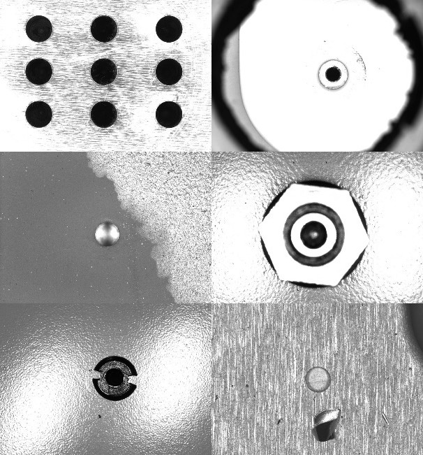
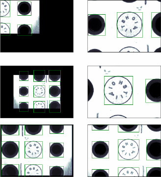
After removing out-of-focus, erroneous images and those not containing any element to be detected, a set of 24625 images was obtained. All the images in the dataset were captured on the gray scale, with a resolution of 5 or 10 MPx. Figure 1 shows some examples of this dataset, in which images from drilling and riveting machines predominate.
Figure 1.
Sample of the images contained in the dataset.
3.1.1Image process and labeling
In the analyzed set of images, different fastening or referencing elements used in aeronautical manufacturing processes were detected and classified into eight different categories (Fig. 2):
a) Drill (D): encompasses every straight blind or through holes, without countersink
b) Countersink (Cs): comprises those holes with countersink
c) Rivet (R): includes those rivets that are flush with the surface
d) Protruding Rivet (PR): those rivets protruding over the surface
e) Temporary Fastener 1 (F1): this category groups images of the head of a temporary fastener, which will be drilled during a subsequent process to insert a rivet
f) Temporary Fastener 2 (F2): the same as F1 category, but in this case the images of the temporary fastener tail are included
g) Hexagonal (Hx): this category represents those elements with a hexagonal shape
h) Screws (S): images of screws are included in this class
The prevalence of elements from the different categories is not uniform throughout the dataset because the D category is by far the best represented one, while the presence of others like PR, Hx and S is minor in the set of images (Table 1).
Table 1
Amount of elements present in each category
| Category | Code | Number |
|---|---|---|
| Drill | D | 23772 |
| Countersink | Cs | 5572 |
| Rivet | R | 1459 |
| Protruding rivet | PR | 360 |
| Temporary fastener 1 | F1 | 8329 |
| Temporary fastener 2 | F2 | 1382 |
| Hexagonal | Hx | 365 |
| Screw | S | 372 |
| Total | 41611 |
Figure 2.
Prototype elements for the established categories.
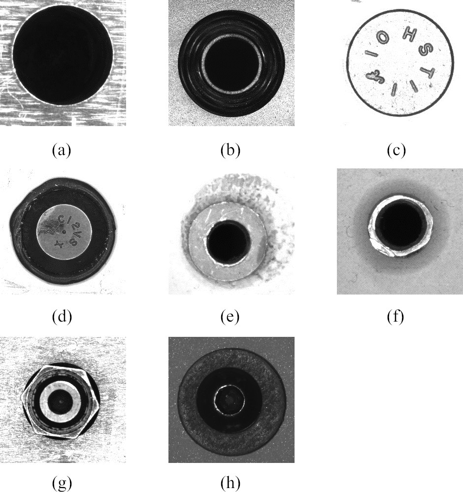
Image labeling was carried out semi-automatically using a potential region proposal algorithm based on the labeling of connected regions (blobs). These proposed regions were subsequently classified with a classification neural network developed in [58].
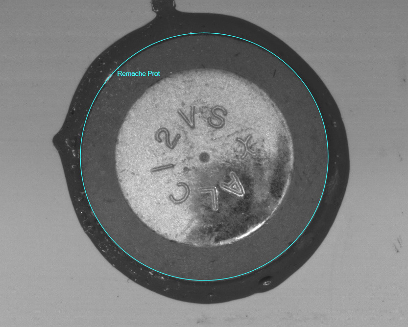
The proposal was finally and manually validated by experts to correct the identification errors made by the automatic labeling algorithm. It should be noted that, given the circular nature of all the identified categories, a decision was made to label these elements by means of the circle that circumscribed them to, thus, do away with the bounding boxes normally used (Fig. 3).
Figure 3.
Element labeling using its circumscribing circle.
3.2Proposed approach
To develop the detection neural network, several of the most widespread architectures were evaluated [59, 60], such as R-CNN, SSD and RetinaNet. Finally, we opted to design a network architecture based on SSD developments [37]. However for this detection problem, a very light convolutional network with only seven layers (inspired by MobileNet architectures [61]) was used as a backbone.
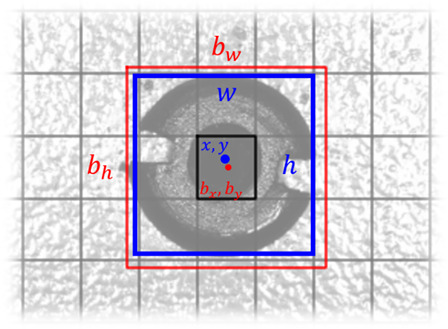
Following the work methodology of SSD networks, the localization of elements was be done in the coordinates related to anchor boxes (represented in Fig. 4). In this case, as the elements to be detected were always circular in nature, their size was characterized by using only the value of their height:
Figure 4.
Element bounding box (blue) and closest anchor box (red).
The neural network structure (shown in Fig. 5) can be divided into three sections:
Figure 5.
Final developed network architecture.
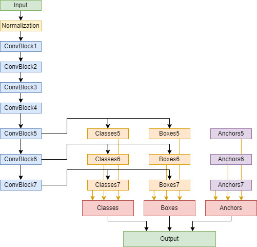
Figure 6.
Accurate measurement “Spoke” algorithm.
An adaptation section or input layer: this section was configured for an image size of 480
Next data were passed through a convolutional section, which constituted the network’s backbone, and was composed of seven convolutional blocks. All these blocks contained a convolutional layer, followed by a Batch Normalization block [62] (with momentum value
Finally, from the last three convolutional blocks, feature maps were extracted (dimensions 30
Additionally, a series of blocks in charge of generating information from anchor boxes was included in the network architecture so that output would contain all the information needed to reconstruct detection values.
All the results of these convolutional blocks were concatenated in the output, whose shape was 815
Instead of following the training scheme proposed for SSD networks, this work opted to do away with the Hard Mining stage and use the FocalLoss function [13] as the primary loss function, parametrized with
3.2.1Measuring fixation elements
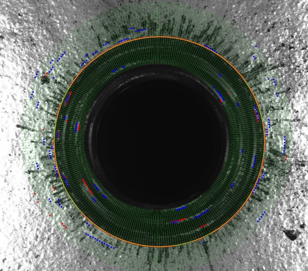
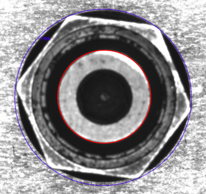
For the accurate adjustment of the center and diameter of referencing elements, a measurement algorithm called Spoke was designed.
The algorithm began by using the circle proposed by the detection neural network (shown in yellow in Fig. 6), on which a set of radii or spokes (drawn in green) was defined and the image intensity values over them were analyzed. These profiles were analyzed during the search of the point of most contrast. For this purpose, the derivative of the values along the profile was calculated. The points with the highest and lowest derivative values (in red and blue, respectively) were, thus, located.
Those points represented the most likely locations of the referencing element edge.
In order to extract the circular shape from the set of points of the highest contrasts, a least squares algorithm to find the circle that best fitted the point set was developed [64].
Given a set of
The value of
where
After calculating the best-fit circle, the root mean square error (RMS) for that solution was calculated. Then a new iteration was executed, when the length of spokes became shorter. This process was run while the RMS value converged, and it stopped when it was lower than a set threshold. If the RMS value did not converge, an early stop would be thrown with a warning for that detection.
This procedure can be used only with the images taken from the perpendicular direction to the plane containing the element, which is the case of all the images in the studied dataset. A more generic approach would require modifying the best-fit algorithm to model an ellipse instead of a circle.
3.3Experimental setup
This study employed 24.6k images (containing 41.6k referencing elements). The images in this dataset were randomized and split into five sets for a K-Fold cross validation (with a training test ratio of 80%–20%). Due to this randomization, the actual ratio test images per class varied between 16% and 23%.
Several data augmentation transformations were randomly applied to the training set of images. The result is shown in Fig. 7:
• Horizontal, vertical symmetry and 180
• Image scaling and translation
• Brightness and contrast transformations
• Image blur
Figure 7.
Examples of the random transformations applied to a single image.
The model was initialized with random values following a truncated normal distribution. Tensorflow’s “HeNormal” initializer [64] was trained and evaluated using machine learning frameworks Tensorflow 2 and Keras. An Adam optimizer [65] was employed for 400 epochs of 100 iterations each at an initial learning rate of
3.3.1Quality factor for result evaluations
Table 2
Quality factor values for several error and diameter settings
| Center quality factor | Diameter quality factor | |||||||||
| Error (mm) | Diameter (mm) | Diameter (mm) | ||||||||
| 4 | 6 | 8 | 10 | 12 | 4 | 6 | 8 | 10 | 12 | |
| 0.01 | 99% | 100% | 100% | 100% | 100% | 100% | 100% | 100% | 100% | 100% |
| 0.02 | 99% | 99% | 99% | 99% | 100% | 99% | 99% | 100% | 100% | 100% |
| 0.05 | 96% | 98% | 98% | 99% | 99% | 98% | 98% | 99% | 99% | 99% |
| 0.1 | 93% | 95% | 96% | 97% | 98% | 95% | 97% | 98% | 98% | 98% |
| 0.2 | 86% | 90% | 93% | 94% | 95% | 90% | 94% | 95% | 96% | 97% |
| 0.5 | 69% | 78% | 83% | 86% | 88% | 78% | 85% | 88% | 90% | 92% |
| 1 | 47% | 61% | 69% | 74% | 78% | 61% | 72% | 78% | 82% | 85% |
| 2 | 22% | 37% | 47% | 55% | 61% | 37% | 51% | 61% | 67% | 72% |
| 5 | 2% | 8% | 15% | 22% | 29% | 8% | 19% | 29% | 37% | 43% |
Figure 8.
Example of the evolution of neural network training and test losses.
The correct categorization of the detected elements was checked by using the confusion matrix, as well as the resulting precision and recall values for each category.
To evaluate neural network performance for correctly locating the referencing elements, an ad hoc metric was designed to assign a value within the interval [0, 1] according to the quality of the performed detection.
For this purpose, two error values were calculated for each detected element (of circular nature) according to the deviation from the center and the deviation in diameter:
where
where coefficients
Table 3
False positive rate per class
| FP relative rate (%) | |
|---|---|
| D | 17.7 |
| Cs | 72.2 |
| R | 1.3 |
| PR | 0.4 |
| F1 | 4.7 |
| F2 | 0.0 |
| Hx | 0.4 |
| S | 3.3 |
Table 4
Global confusion matrix
| Predicted Class (%) | ||||||||||
|---|---|---|---|---|---|---|---|---|---|---|
| FN | D | Cs | R | PR | F1 | F2 | Hx | S | ||
| Ground | D | 2.29 | 97.50 | 0.16 | 0.01 | 0.00 | 0.03 | 0.00 | 0.00 | 0.00 |
| truth | Cs | 6.15 | 2.92 | 90.87 | 0.00 | 0.00 | 0.04 | 0.02 | 0.00 | 0.00 |
| R | 9.84 | 0.00 | 0.00 | 90.16 | 0.00 | 0.00 | 0.00 | 0.00 | 0.00 | |
| PR | 4.31 | 0.00 | 0.00 | 1.19 | 94.50 | 0.00 | 0.00 | 0.00 | 0.00 | |
| F1 | 0.75 | 0.09 | 0.07 | 0.00 | 0.00 | 99.03 | 0.06 | 0.00 | 0.00 | |
| F2 | 4.24 | 0.14 | 0.00 | 0.00 | 0.00 | 0.15 | 95.47 | 0.00 | 0.00 | |
| Hx | 9.68 | 0.00 | 0.00 | 0.00 | 0.00 | 0.00 | 0.00 | 90.32 | 0.00 | |
| S | 10.55 | 0.00 | 0.00 | 0.00 | 0.00 | 0.00 | 0.00 | 0.00 | 89.45 | |
Table 2 outlines the calculated quality factor values for several configurations.
In both cases, three areas were defined for the quality of the detected elements:
Considering the global quality factor, which was calculated the multiplication of both individual values, the corresponding ranges were:
• Very good (upright):
• Medium (bold): 90%
• Bad (italic):
4.Results
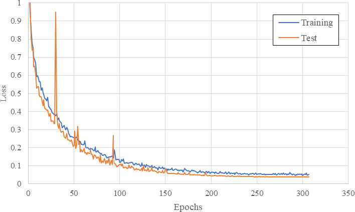
With the described configuration, neural network training was executed for 307 epochs. Then the established early stopping mechanism was activated (Fig. 8).
Once training ended, network performance in the test set was evaluated for the different detection threshold values (every detected element was given a confidence value, but only those with a value above the threshold were considered actual detections. This value helps to balance network sensitivity). The best results were obtained within the range of the detection threshold values [0.55, 0.75]. Specifically, the maximum of parameter F1 (defined as the harmonic mean of precision and recall [66], averaged over 5 folds) was reached for a value of 0.58, with which a 1.25% false-positive (PF) rate and a 1.34% false-negative (FN) rate would be obtained. In the studied case, as FPs in detection were severer (and could lead to the erroneous drilling of the part) than FNs, a detection threshold of 0.70 was selected, which gave FP and FN rates of 0.58% and 2.97%, respectively.
The rate of FP detections was split into the different classes shown in Table 3.
Table 5
Quality factors in the neural network localization
| Raw NN output (%) | Spoke refinement (%) | |||||||
| Class |
|
|
|
|
|
| ||
| D | 92.87 | 94.80 | 88.04 | 99.58 | 99.40 | 98.99 | ||
| Cs | 90.56 | 88.54 | 80.19 | 97.66 | 94.20 | 91.99 | ||
| R | 86.40 | 86.09 | 74.38 | 95.44 | 89.97 | 85.86 | ||
| PR | 90.62 | 90.03 | 81.58 | 98.46 | 55.12 | * | 54.27 | * |
| F1 | 93.66 | 93.11 | 87.20 | 98.00 | 95.18 | 93.28 | ||
| F2 | 92.72 | 91.21 | 84.57 | 97.11 | 86.75 | 84.25 | ||
| Hx | 83.37 | 81.14 | 67.65 | 90.34 | 26.90 | * | 24.30 | * |
| S | 87.10 | 88.44 | 77.04 | 95.65 | 90.38 | 86.45 | ||
| Global | 92.35 | 93.00 | 85.89 | 99.24 | 98.15 | 97.40 | ||
The system’s accuracy for locating and measuring the diameter of the detected elements was also evaluated (Table 5). This evaluation, averaged over 5 folds, was done for the raw output of the neural network and after applying the Spoke algorithm to allow the improvement introduced into the system by this algorithm to be evaluated.
Figure 9.
Examples of detecting referencing elements.
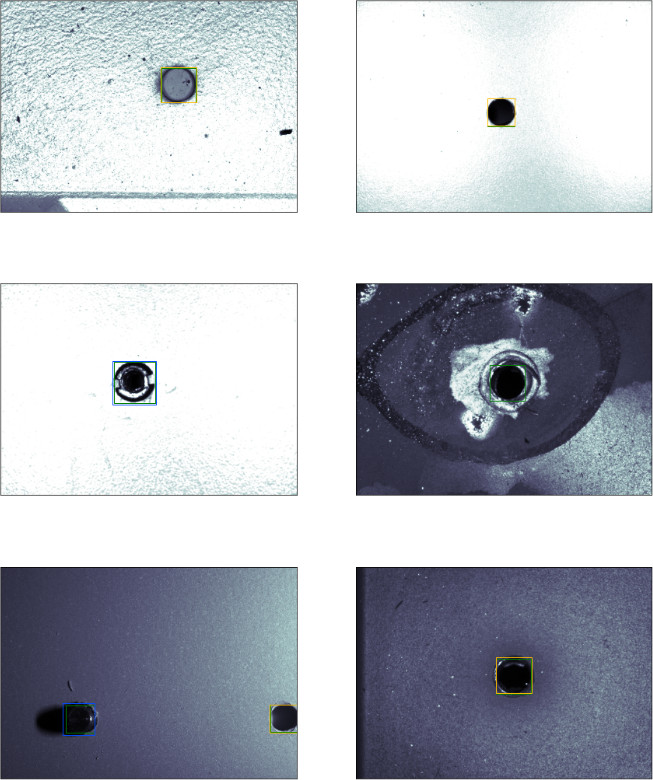
Figure 10.
Discrepancy between the bounding box defined for training (blue) and the circle optimized by the Spoke algorithm (red).
Finally, some examples of detection carried out by the neural network are presented in Fig. 9.
The evaluation of the quality factors deserves special attention for classes PR and Hx because their measured diameter did not match that detected by the network (Fig. 10). This situation is further explained in Section 5.
4.1Ablation study
The performance improvement achieved by the replacement of the original SSD training scheme with Focal Loss training was studied. To do so, a network was trained following this original scheme.
In this network, the detection threshold was adjusted so that the same FP rate would be achieved (0.58%). For this threshold, the network returned a bigger FN number (3.70%).
Classification accuracies were similar for every class, except for S class, where 90.0% of the elements were not detected (FN), and the remaining 9.1% were incorrectly assigned to other categories.
This test clearly showed how using Focal Loss with this architecture improved the management of the unbalanced datasets, and no further actions were needed. Regarding the location accuracy of the detected elements, the averaged values of
5.Discussion
With the chosen configuration and overall FP and FN rates of 0.35% and 2.36% respectively, the classification accuracy over the detected elements was higher than 90% in most categories, despite the disparity in the number of examples between the different categories. This revealed that class unbalance was correctly managed by the selected loss function.
The classes with a higher rate of FN detections were S, R and Hx (around 10%). The FPs shown in the results comprised mainly elements from classes Cs (72%) and D (18%). Both situations could be explained by the relative number of elements in each class.
By considering the classification accuracy among classes, only Cs and PR showed significant classification errors, where around 3% of the Cs elements were misclassified as D and 1.2% of PR were incorrectly classified as R. These errors could be explained by the similarity between these classes (countersink-straight drill, rivet-protruding rivet).
The neural network accuracy in element localization terms yielded an average quality factor of 92.5% for localization and 93.6% for the diameter measurement. This is the equivalent to position and diameter errors of 0.21 mm and 0.26 mm, respectively, for an 8-mm diameter element. However, they are insufficient values for the precision required in aeronautical manufacturing processes.
By subsequently executing the Spoke algorithm, it was possible to increase these accuracies to an average value of 98.5% for location and 97.3% for the diameter measurement. These values are the equivalent to errors of 0.04 mm and 0.11 mm, respectively, which are sufficiently accurate for the aforementioned manufacturing processes.
The diameter quality factor calculation gave inconsistent results in Hx and PR. This was because the bounding box selected for training (which circumscribes the element to be detected) did not fulfill the geometric and contrast requirements needed by the Spoke algorithm to accurately locate the element. As a workaround for these categories, an inner concentric circular shape was chosen by selecting a smaller circle as a seed for the algorithm. This choice gave accurate center results, but the quality factor for the diameter was distorted in the results. An example of this situation is illustrated in Fig. 10.
With the aforementioned configuration, the training time of the neural network was under 7 h, with an average training time of about 78 seconds per epoch.
In turn, the prediction of an image took the system about 3.5 ms, while the refinement of detection using the Spoke algorithm needed about 20–24 ms.
6.Conclusions
A novel system has been developed for the detection and accurate measurement of referencing elements in industrial environments of aeronautical manufacturing processes, which lowers FP and FN rates in relation to conventional systems and, thus, improves the reliability of inspection processes.
The reduction in the FN rate also involved needing fewer manual interventions to complete the manufacturing process, which increases process productivity. The reduction in FPs in detection translates meant fewer erroneous operations in the system, which lowers final manufacturing costs.
The developed system was integrated into a real production environment with a manual intervention rate of operators of 13.3% (due to the detection errors of the previous algorithm based on detection and filtering by blobs), which was a drastic reduction and gave a new manual intervention rate of only 0.6%.
Future developments will work on integrating the Spoke measurement algorithm into the neural network architecture itself to make the most of these systems’ parallel processing power, which allows more accurate measurements in complex scenes.
Funding
This publication has been carried out within the frame-work of Project “Nuevas Uniones de estructuras aeronáuticas”, reference number IDI-20180754. This project has been supported by the Spanish Ministry of Science and Technology and the Centre for Industrial Technological Development (CDTI).
References
[1] | Deloitte. 2022 Aerospace and defense industry outlook. (2022) . |
[2] | Devlieg R. Expanding the use of robotics in airframe assembly via accurate robot technology. SAE Int J Aerospace. (2010) ; 3: (1): 198-203. |
[3] | Barbosa G, Aroca R. Advances of Industry 4.0 concepts on aircraft construction: an overview of trends. J Steel Struct Constr. (2017) ; 3: : 125. |
[4] | Crandall DJ. Artificial intelligence and manufacturing. Smart Factories: Issues of Information Governance. (2019) ; 10-6. |
[5] | Gramegna N, Corte ED, Cocco M, Bonollo F, Grosselle F, editors. Innovative and integrated technologies for the development of aeronautic components. TMS Annual Meeting. (2010) . |
[6] | Ahmad HM, Rahimi A. Deep learning methods for object detection in smart manufacturing: A survey. Journal of Manufacturing Systems. (2022) ; 64: : 181-96. |
[7] | Kotsiopoulos T, Sarigiannidis P, Ioannidis D, Tzovaras D. Machine Learning and Deep Learning in smart manufacturing: The Smart Grid paradigm. Computer Science Review. (2021) ; 40: : 100341. |
[8] | Yang J, Li S, Wang Z, Dong H, Wang J, Tang S. Using deep learning to detect defects in manufacturing: a comprehensive survey and current challenges. Materials. (2020) ; 13: (24): 5755. |
[9] | Bordel B, Alcarria R, Robles T. Recognizing human activities in Industry 4.0 scenarios through an analysis-modeling- recognition algorithm and context labels. Integrated Computer-Aided Engineering. (2022) ; 29: (1): 83-103. |
[10] | Bordel B, Alcarria R, Robles T. Lightweight encryption for short-range wireless biometric authentication systems in Industry 4.0. Integrated Computer-Aided Engineering. (2022) ; 29: (2): 153-73. |
[11] | Roda-Sanchez L, Olivares T, Garrido-Hidalgo C, De La Vara JL, Fernandez-Caballero A. Human-robot interaction in Industry 4.0 based on an Internet of Things real-time gesture control system. Integrated Computer-Aided Engineering. (2021) ; 28: (2): 159-75. |
[12] | Bauer JM, Bas G, Durakbasa NM, Kopacek P, editors. Development Trends in Automation and Metrology. IFAC-PapersOnLine. (2015) . |
[13] | Mei Z, Maropoulos PG. Review of the application of flexible, measurement-assisted assembly technology in aircraft manufacturing. Proceedings of the Institution of Mechanical Engineers, Part B: Journal of Engineering Manufacture. (2014) ; 228: (10): 1185-97. |
[14] | Barbedo JGA. A Review on the Use of Computer Vision and Artificial Intelligence for Fish Recognition, Monitoring, and Management. Fishes. (2022) ; 7: (6). |
[15] | Malik K, Robertson C, Roberts SA, Remmel TK, Long JA. Computer vision models for comparing spatial patterns: understanding spatial scale. International Journal of Geographical Information Science. (2023) ; 37: (1): 1-35. |
[16] | Silva JL, Bordalo R, Pissarra J, de Palacios P. Computer Vision-Based Wood Identification: A Review. Forests. (2022) ; 13: (12). |
[17] | Zhang Y, Lin W. Computer-vision-based differential remeshing for updating the geometry of finite element model. Computer-Aided Civil and Infrastructure Engineering. (2022) ; 37: (2): 185-203. |
[18] | Ngeljaratan L, Moustafa MA, Pekcan G. A compressive sensing method for processing and improving vision-based target-tracking signals for structural health monitoring. Computer-Aided Civil and Infrastructure Engineering. (2021) ; 36: (9): 1203-23. |
[19] | Sajedi SO, Liang X. Uncertainty-assisted deep vision structural health monitoring. Computer-Aided Civil and Infrastructure Engineering. (2021) ; 36: (2): 126-42. |
[20] | Ma Z, Choi J, Soh H. Real-time structural displacement estimation by fusing asynchronous acceleration and computer vision measurements. Computer-Aided Civil and Infrastructure Engineering. (2022) ; 37: (6): 688-703. |
[21] | Mileski YR, Souza AJ, Amorim HJ. Development of a computer vision-based system for part referencing in CNC machining centers. Journal of the Brazilian Society of Mechanical Sciences and Engineering. (2022) ; 44: (6): 243. |
[22] | Sinha A, Aneesh RP, Nazneen NS, editors. Eye Tumour Detection Using Deep Learning. Proceedings of 2021 IEEE 7th International Conference on Bio Signals, Images and Instrumentation, ICBSII 2021. (2021) . |
[23] | Huan L, Li W, Yujian Q, editors. Vehicle Logo Retrieval Based on Hough Transform and Deep Learning. In: Proceedings – 2017 IEEE International Conference on Computer Vision Workshops, ICCVW 2017. (2017) . |
[24] | Liang Q, Long J, Nan Y, Coppola G, Zou K, Zhang D, et al. Angle aided circle detection based on randomized Hough transform and its application in welding spots detection. Mathematical Biosciences and Engineering. (2019) ; 16: (3): 1244-57. |
[25] | Ercan MF, Qiankun AL, Sakai SS, Miyazaki T, editors. Circle detection in images: A deep learning approach. In: 2020 Global Oceans 2020: Singapore - US Gulf Coast. (2020) . |
[26] | Mekhalfi ML, Nicolo C, Bazi Y, Rahhal MMA, Alsharif NA, Maghayreh EA. Contrasting YOLOv5, Transformer, and EfficientDet Detectors for Crop Circle Detection in Desert. IEEE Geoscience and Remote Sensing Letters. (2022) ; 19: . |
[27] | Xia X, Liang H, Rongfeng Y, Kun Y, editors. Oil Tank Extraction in High-Resolution Remote Sensing Images Based on Deep Learning. In: International Conference on Geoinformatics. (2018) . |
[28] | Zalpour M, Akbarizadeh G, Alaei-Sheini N. A new approach for oil tank detection using deep learning features with control false alarm rate in high-resolution satellite imagery. International Journal of Remote Sensing. (2020) ; 41: (6): 2239-62. |
[29] | Zhu Y, Moayed Z, Bollard-Breen B, Doshi A, Ramond JB, Klette R, editors. Detection of Fairy Circles in UAV Images Using Deep Learning. In: Proceedings of AVSS 2018 – 2018 15th IEEE International Conference on Advanced Video and Signal-Based Surveillance. (2019) . |
[30] | Qin P, Wang L, Lv H, editors. Optic disc and cup segmentation based on deep learning. In: Proceedings of 2019 IEEE 3rd Information Technology, Networking, Electronic and Automation Control Conference, ITNEC 2019. (2019) . |
[31] | Judt D, Lawson C, Van Heerden ASJ. Rapid design of aircraft fuel quantity indication systems via multi-objective evolutionary algorithms. Integrated Computer-Aided Engineering. (2021) ; 28: (2): 141-58. |
[32] | Martins GB, Papa JP, Adeli H. Deep learning techniques for recommender systems based on collaborative filtering. Expert Systems. (2020) ; 37: (6): e12647. |
[33] | Girshick R, editor. Fast R-CNN. In: 2015 IEEE International Conference on Computer Vision (ICCV). (2015) December 7-13. |
[34] | Girshick R, Donahue J, Darrell T, Malik J, editors. Rich feature hierarchies for accurate object detection and semantic segmentation. In: Proceedings of the IEEE Computer Society Conference on Computer Vision and Pattern Recognition. (2014) . |
[35] | He K, Zhang X, Ren S, Sun J, editors. Deep Residual Learning for Image Recognition. In: 2016 IEEE Conference on Computer Vision and Pattern Recognition (CVPR) (2016) June 27-30. |
[36] | Lin TY, Goyal P, Girshick R, He K, Dollár P, editors. Focal Loss for Dense Object Detection. In: 2017 IEEE International Conference on Computer Vision (ICCV) (2017) October 22-29. |
[37] | Liu W, Anguelov D, Erhan D, Szegedy C, Reed S, Fu C-Y, et al., editors. SSD: Single Shot MultiBox Detector. In: Computer Vision – ECCV 2016. Cham: Springer International Publishing; (2016) . |
[38] | Redmon J, Divvala S, Girshick R, Farhadi A. You Only Look Once: Unified, Real-Time Object Detection. (2016) . |
[39] | Ren S, He K, Girshick R, Sun J. Faster R-CNN: Towards Real-Time Object Detection with Region Proposal Networks. IEEE Transactions on Pattern Analysis and Machine Intelligence. (2017) ; 39: (6): 1137-49. |
[40] | Simonyan K, Zisserman A. Very deep convolutional networks for large-scale image recognition. arXiv preprint arXiv:14091556. (2014) . |
[41] | Wang C-Y, Bochkovskiy A, Liao H-YM. YOLOv7: Trainable bag-of-freebies sets new state-of-the-art for real-time object detectors. arXiv preprint arXiv:220702696. (2022) . |
[42] | Hassanpour A, Moradikia M, Adeli H, Khayami SR, Shamsinejadbabaki P. A novel end-to-end deep learning scheme for classifying multi-class motor imagery electroencephalography signals. Expert Systems. (2019) ; 36: (6): e12494. |
[43] | Tan M, Pang R, Le QV, editors. EfficientDet: Scalable and Efficient Object Detection. In: 2020 IEEE/CVF Conference on Computer Vision and Pattern Recognition (CVPR) (2020) June 13-19. |
[44] | Cai Z, Fan Q, Feris R, Vasconcelos N. A Unified Multi-scale Deep Convolutional Neural Network for Fast Object Detection. (2016) . |
[45] | Macias-Garcia E, Galeana-Perez D, Medrano-Hermosillo J, Bayro-Corrochano E. Multi-stage deep learning perception system for mobile robots. Integrated Computer-Aided Engineering. (2021) ; 28: (2): 191-205 |
[46] | Benamara NK, Val-Calvo M, Álvarez-Sánchez JR, Díaz-Morcillo A, Ferrández-Vicente JM, Fernández-Jover E, et al. Real-time facial expression recognition using smoothed deep neural network ensemble. Integrated Computer-Aided Engineering. (2021) ; 28: (1): 97-111. |
[47] | Gąsienica-Józkowy J, Knapik M, Cyganek B. An ensemble deep learning method with optimized weights for drone-based water rescue and surveillance. Integrated Computer-Aided Engineering. (2021) ; 28: (3): 221-35. |
[48] | Bochkovskiy A, Wang C-Y, Liao H-Y. YOLOv4: Optimal Speed and Accuracy of Object Detection. (2020) . |
[49] | Redmon J, Farhadi A. YOLOv3: An Incremental Improvement. (2018) . |
[50] | Lin T-Y, Goyal P, Girshick R, He K, Dollár P, editors. Focal loss for dense object detection. In: Proceedings of the IEEE International Conference on Computer Vision. (2017) . |
[51] | Kussul N, Lavreniuk M, Skakun S, Shelestov A. Deep Learning Classification of Land Cover and Crop Types Using Remote Sensing Data. IEEE Geoscience and Remote Sensing Letters. (2017) ; 14: (5): 778-82. |
[52] | Gómez-Silva MJ, De La Escalera A, Armingol JM. Back-propagation of the Mahalanobis istance through a deep triplet learning model for person Re-Identification. Integrated Computer-Aided Engineering. (2021) ; 28: (3): 277-94. |
[53] | Nogay S, Adeli H. Diagnostic of autism spectrum disorder based on structural brain MRI images using, grid search optimization, and convolutional neural networks. Biomedical Signal Processing and Control. (2023) ; 79: : 104234. |
[54] | Nogay HS, Adeli H. Detection of Epileptic Seizure Using Pretrained Deep Convolutional Neural Network and Transfer Learning. European Neurology. (2020) ; 83: (6): 602-14. |
[55] | Chen Y, Jiang H, Li C, Jia X, Ghamisi P. Deep Feature Extraction and Classification of Hyperspectral Images Based on Convolutional Neural Networks. IEEE Transactions on Geoscience and Remote Sensing. (2016) ; 54: (10): 6232-51. |
[56] | Schmidt C, Hocke T, Denkena B. Deep learning-based classification of production defects in automated-fiber-placement processes. Production Engineering. (2019) ; 13: (3): 501-9. |
[57] | Schmidt C, Hocke T, Denkena B. Artificial intelligence for non-destructive testing of CFRP prepreg materials. Production Engineering. (2019) ; 13: (5): 617-26. |
[58] | Ruiz L, Torres M, Gómez A, Díaz S, González JM, Cavas F. Detection and Classification of Aircraft Fixation Elements during Manufacturing Processes Using a Convolutional Neural Network. Applied Sciences. (2020) ; 10: (19). |
[59] | Jiao L, Zhang F, Liu F, Yang S, Li L, Feng Z, et al. A Survey of Deep Learning-Based Object Detection. IEEE Access. (2019) ; 7: : 128837-68. |
[60] | Jodas DS, Yojo T, Brazolin S, Velasco GDN, Papa JP. Detection of Trees on Street-View Images Using a Convolutional Neural Network. International Journal of Neural Systems. (2022) ; 32: (1): 2150042. |
[61] | Howard AG, Zhu M, Chen B, Kalenichenko D, Wang W, Weyand T, et al. Mobilenets: Efficient convolutional neural networks for mobile vision applications. arXiv preprint arXiv:170404861. (2017) . |
[62] | Ioffe S, Szegedy C, editors. Batch normalization: Accelerating deep network training by reducing internal covariate shift. In: International Conference on Machine Learning. PMLR; (2015) . |
[63] | Ghilani CD. Adjustment computations: spatial data analysis. John Wiley & Sons; (2017) . |
[64] | He K, Zhang X, Ren S, Sun J, editors. Delving Deep into Rectifiers: Surpassing Human-Level Performance on ImageNet Classification. In: 2015 IEEE International Conference on Computer Vision (ICCV). (2015) December 7-13. |
[65] | Kingma DP, Ba J. Adam: A method for stochastic optimization. arXiv preprint arXiv:14126980. (2014) . |
[66] | Taha AA, Hanbury A. Metrics for evaluating 3D medical image segmentation: analysis, selection, and tool. BMC Medical Imaging. (2015) ; 15: (1): 29. |


