An efficient multi-robot path planning solution using A* and coevolutionary algorithms

1.Introduction

Technological advances make the management of logistic centers easier by using robots in the transportation tasks, either with homogeneous or heterogeneous robots [1]; in this study, we restrict ourselves to this latter category, with all the robots moving in the same common space, with same type of movements and the same speed. The problem of determining the best route for each robot moving in a shared space without collisions nor human intervention is known as collision Free Multi-robot Path Planning (MPP). MPP has applications in multiple fields such as intelligent laboratories[2, 3], space exploration [4], warehouse management [5], education [3], surveillance [6], manufacturing [7], unmanned aerial vehicles [6, 8, 9, 10], and many others.

In a MPP problem, each robot moves from its initial point -either in a depot or in a free parking area- to their current destination on a common workspace. It has been shown that, although a NP-problem [11], optimization techniques can solve it effectively [12, 13]. The most cited algorithm used in single-robot path planning is A* [14], that is, A* determines the optimal route for a robot from its initial position to its goal. Since its introduction, several different alternative algorithms have been proposed to cope with the MPP problem: Collaborative A*, Hierarchical Collaborative A* (HCA*) and Windowed HCA* [15], D*Lite[16], Field D* [17], ThetA* [18], M* [19, 20], Operator Decomposition [21] and Independence Detection [22]. These algorithms determine the collisions, finding alternative routes by searching the graph representation of the problem. Some of them calculate direct and linear routes -without constraining to grid edges (i.e., ThetA* or Field-D*), some others (D*Lite or Field D*, for instance) avoid collisions on the fly by detecting them and recalculating the routes; all of these approaches are, in general, oriented towards autonomous robot navigation. For a comparison of these algorithms with and without meta-heuristics, please refer to [23, 24, 25].

A different alternative is proposed in [26], where a construction of a mixed-split graph for every two connected nodes is used; a new extended version of the original graph is constructed by repeating this structure T times -with T the expected time of arrival- and introducing extra edges representing whether a robot stays in its node or moves to the next one. Then, a linear programming algorithm is used to determine the route for each robot. Finally, the constrain based search was proposed in [27], with two abstraction layers: on the high level, agents with collision free routes are found, for each one searches on the low level are performed until a feasible combination is determined.

Optimization metaheuristics have been found performing similarly or better than classical methods for the MPP problem [23]; in this study, a comparison of different alternatives, including Genetic Algorithms (GA), Differential Evolution (DE), Particle Swarm Optimization (PSO), Cuckoo Search, or the Dijkstra algorithm, among others. In [28], Ant Colony Optimization (ACO) has been reported for determining the optimal routes. An hybridization of PSO and Gray-Wolf Optimization has been proposed in [29], relying the collision detection to local resolutions using the robot sensory system and local search. Similarly, the studies in [30, 31, 32] split the problem in two: a centralized stage determining the optimal routes for each robot and a decentralized stage in charge of solving the collisions. To do so, the authors in [30] proposed solving some linear equations based on constraints related with the robot goals, while in [31] the authors proposed to use Lion Optimization for this decoupled task. In contrast, DE was proposed as the main heuristic in [32].

PSO has not only been applied by itself to the MPP problem, but also hybridized with other techniques, such as differential perturbed velocity [33] or gravitational search [34]. Authors in [35] solved the path planning problem based on a two-step process: the first makes use of Artificial Potential Fields (APF) to generate the initial feasible routes, and then, the second stage uses of GA in order to optimize the paths and collision avoidance. Similarly, [36] solves MPP problems using APF and fuzzy inference systems. Not related with metaheuristics but worth mentioning is the use of Reinforcement Learning for MPP [37, 38].

This study is restricted to grid-based problems, such as warehouses or virtual remote labs, where the space is represented by means of a grid and, mainly, the 4-way connectivity rule [39]. Applied in this context, Windowed Hierarchical Cooperative A* (WHCA*) has been employed in solving the MPP using the number of turns as heuristic for the A* algorithm [40]. On the other hand, the capability of D*Lite to cope with a changing environment is used in [41] for solving a warehouse MPP problem. The same problem is addressed for a warehouse in [5], where a specific algorithm is develop determining some intermediate points and joining them with straight lines. A different proposal is presented in [39, 42], using the so-called DDM algorithm (Diversified-path Database-driven Multi-robot Path Planning) able to compute near-optimal solutions to large-scale MPP. DDM follows the decoupled paradigm and first creates a shortest path for each robot from its initial vertex to goal vertex, ignoring other robots. Then, a simulated execution is carried out. As conflicts are detected, they are solved within local sub-graphs with the help of the main heuristics. Similarly, two coordinated layers are proposed in [43] for solving the MPP problem in an industrial warehouse: one layer focuses on the abstract representation of the problem, and the second one focuses on determining the paths. A very similar approach is reported in [44], dividing the warehouse in sectors; a top layer determines the number of vehicles in each sector, while A* with conflict-based searching strategy is used in the path generation at the lowest coordination level.

In this research, a metaheuristic based solution for the MPP problem is proposed, enhancing our previous research results reported in [45]. The solution construction is split in three stages: firstly, an A* initial optimal route finding process is performed, followed by an A*-based alternatives search, and finalizing with a co-evolutionary optimization process that examines and modifies the available pool of routes among all the conflicting robots until a feasible solution is found. This research solves the high computational cost issues reported in the initial research, greatly improving the performance and making it capable of solving problems faster and with a significantly higher number of robots.

The structure of this documents is as follows. Section 2 explains the proposal, remarking the differences with the previous research. Next, Section 3 gives details of the experimentation set up, while Section 4 shows the results and discussion. Finally, Section 5 draws the conclusions extracted from this study.

2.A collision free multi-robot path planning proposal

This proposal focuses on MPP in grid-mapped environments represented as {M, R, S, G}, where M is the map of the environment stored as a 2D graph where the robots are located in and including the obstacles, R is the set of robots {r1, …, rN}. The initial and ending locations of the robots (S = {s1, …, sN} and G = {g1, …, gN}, respectively) are also given. The objective of the problem is to provide a collision-free route for each of the robots.

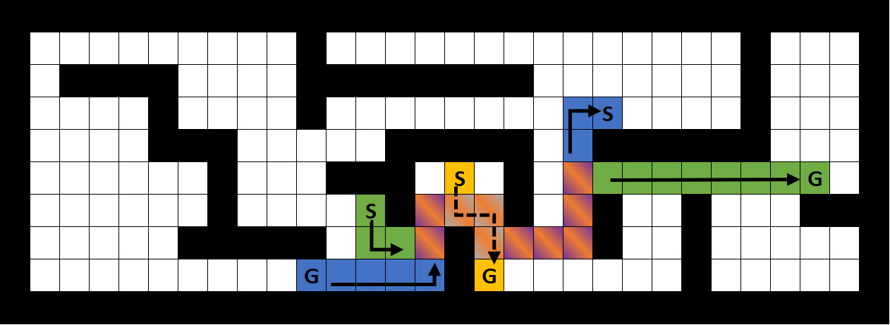
Figure 1.

A simple example of a maze representation of a problem. The path for the blue, yellow and green robots (colored squares) from their starting points to their goals (colored circles) are LDDDDLLULLDDLLL, DRDD and DRRURRDRUURRRRRRR, correspondingly, assuming (L)eft, (R)ight, (U)p and (D)own movements.

Let us denote by δ is the set of valid movement operations. A movement operation δi is one of the unitary movements the robot can perform in a time unit; for the purpose of this study, δ= {(H)alt, (U)p, (D)own, (L)eft, (R)ight} are the available movements as explained in [39]. Figure 1 gives an example of a maze with 3 robots (blue, green and yellow), their shortest routes and the routes’ representation. The starting and ending cells are denoted with a circle and a square, respectively; the cell pattern is marked with a grid and the obstacles are the black cells. As it can be seen, the robots’ routes share some cells; if this sharing coincides in time we get a collision. For the sake of simplicity, we assume that there are no pending trajectories in development, that is, there are no other robots already moving in the scenario. Nevertheless, this can be easily introduced as well, so the new routes could be completely compatible with those previously delivered and in action.

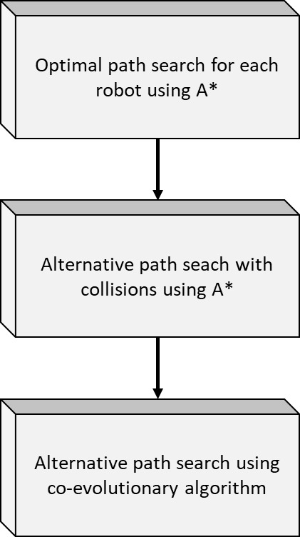
To solve the MPP problem a three stages procedure is proposed (see Fig. 2 and Algorithm 2): i) searching for optimal path for each robot using A*, ii) searching for alternative paths for robots with collisions using A*, and iii) producing feasible paths using a co-evolutionary algorithm.

Figure 2.

Block diagram of the proposed approach for solving the MPP.

General algorithmeach robot r Calculate the A* route Detect collisions as explained in [15]There exist any collision Alternative path search Co-evolutionary collision resolution

Basically, the first stage runs the A* algorithm for each robot, so an initial optimal set of routes is available; however, these routes might collide and alternatives are searched in the remaining two stages. The next subsections explain these two stages; a final subsection is devoted to remark the differences with our previous research.

2.2Co-evolutionary algorithm for collision resolution

The co-evolutionary algorithm is the responsible of finding new routes for those colliding persistent robots, those whose (n⁢A+1) routes from previous stages still keep colliding with other robots. In this research we propose to use a co-evolutionary algorithm for this purpose because we can evolve the routes from each colliding robot independently; furthermore, the robots can collaborate with the others by sharing their collection of routes. Robots for which a successful route was found in the previous stage are kept constant and no modifications to their routes are introduced.

Although it would be much faster if we select one colliding robot -that of smallest number of collisions- to be also kept constant and finding routes for the remaining ones, we decided against it because cross-collisions might lead to introduce more heuristics in the selection of the optimal robot to be kept fixed. Given that the low convergence speed of co-evolutionary algorithms, we chose to avoid this stage introducing all colliding robot in the process.

The next subsections describe the co-evolutionary design, the co-evolutionary evaluation, and the co-evolutionary process.

2.2.1The co-evolutionary design

In a co-evolutionary algorithm we keep several populations that evolve independently, sharing their effort to obtain a valid final global solution. In this study, a populationPr keeps a collection of size Lr of the most plausible routes for the colliding robot r. Besides, an individual in the population represents a route for a robot, with its initial sr and final gr positions plus a character string describing the path as a sequence of movements δir∈δ, as shown in Fig. 1. During the evolutionary process only the data concerning the movements can be modified.

The initial population for robot r (P0r) includes the n⁢A routes calculated in the previous stages, plus Lr-n⁢A extra routes generated by applying the mutation operator to one of the already included routes in P0r.

The co-evolutionary scheme makes use of elitism, so the best K individuals from population Pt-1r are copied into the next generation Ptr the population at time t for robot r. Ptr is completed to size Lr using a tournament selection -with probability p set to 0.35- plus the mutation operator. For the purpose of this research, we experimented with the problem in Fig. 1 to set the probability of mutation, finding that this parameter needs to be higher the better, making the optimization more an individual replacement evolutionary process with an elite population which actually makes sense with the proposal of finding more new alternatives. The algorithm for the generation of the new population is shown in Algorithm 2.2.1.

Generation of a populationSelect the best individuals to keep as the elite subpopulation next population is not complete Select the parent individual for evolution using tournament Apply mutation to the parent individual resulting a new individual the new individual is valid Introduce it in the new population

The mutation operator performs a minor modification on an existing route in the population, generating a new route; the process is illustrated in Figs 3 and 4. The mutation operator randomly selects a Mutation Start Point (MSP). Then, a movement δMSPr must be randomly chosen from the five valid movements in δ: up (U), down (D), left (L), right (R), or halt (H). The selected operation will be introduced into the route at the MSP. If the chosen operation halt (H), the new route is already a valid route, and the mutation operator is terminated (Fig. 3).

Figure 3.

Mutation operation when the HALT movement is introduced. The route goes from RRRRRUURRDRRUUUUR to RHRRRRUURRDRRUUUUR.

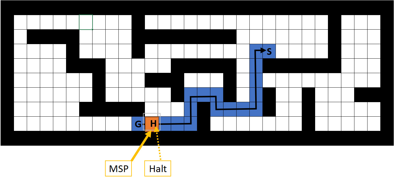
Figure 4.

Mutation operation when two movements are introduced. The route changes from RRRRRUURRDRRUUUUR to RURRRD RUURRDRRUUUUR.

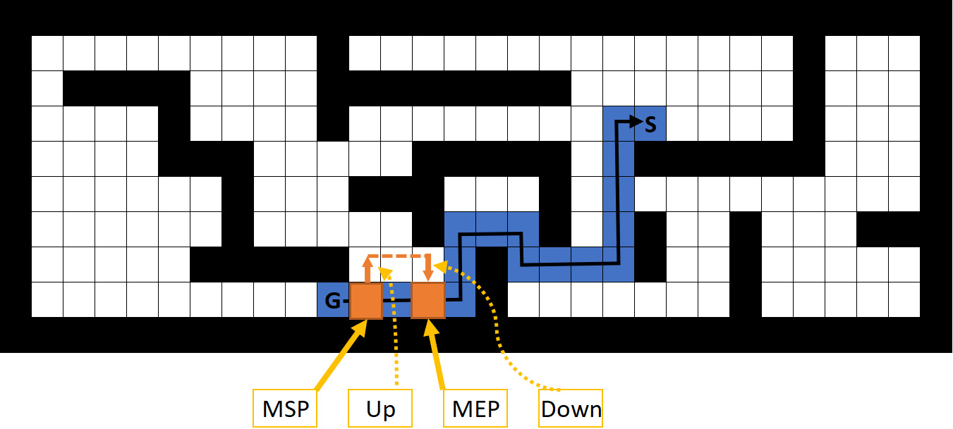
Figure 5.

Mutation operation when only one movement is introduced. The route changes from RRRRRUURRDRRUUUUR to RURRRRURRDRRUUUUR.

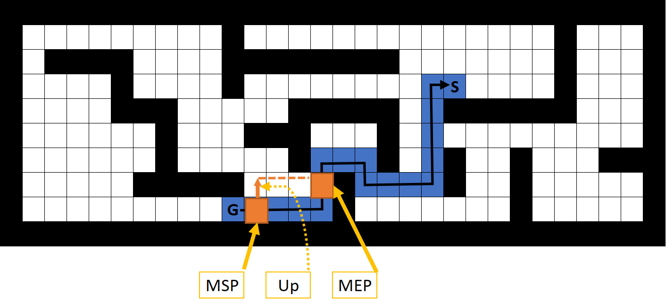
However, if the selected operation is one of the other four movements, a second point called Mutation End Point (MEP) must be selected -which must be after the MSP- where the parent and the offspring paths merges again. The offspring, then, runs parallel to the parent one until the proximity to the MEP. If the two routes (parent and offspring) differs at the MEP in a single cell, the needed movement from δ is introduced in offspring route so both routes merge; this is reflected in Fig. 4. For the remaining cases, the mutated and original paths merge before MEP and no extra movement is required, as shown in Fig. 5.

It is worth noticing that in this research we restrict the MSP to be chosen among the movements before a collision occurs, which reduces the search space. The same can be reasoned for the MEP, so it also must be before the collision occurs.

Finally, the mutation operator considers a different probability for each movement in δ. In this sense, the HALT movement is more likely to reduce collisions; thus, its selection probability is higher, specially when two robots collide in a narrow passage: the optimal solution for this collision could be for one of the robots to stop and wait for the other to clear the corridor, resuming its route just afterwards. Therefore, the probability for the HALT movement is set to 0.6, while each of the remaining movements -Left, Right, Up and Down- has a 0.1 probability of being chosen; these values have been manually selected according to the hypothesis above explained.

2.2.2Co-evolutionary evaluation

There are two co-evolutionary evaluations: the local co-evaluation, which is computed on each individual, and the global evaluation, which is computed for each robot population.

In the local co-evaluation, both the performance and the validity of each individual are evaluated. On the one hand, the performance is evaluated considering two measurements: i) the estimated number of collisions and ii) the length of the routes. While the latter, the length of a route, is just measured as the number of movements composing a path, the former measurement is a bit more complex.

To calculate the estimated number of collisions, firstly, Q routes are selected from each sub-population, with Q taking a relatively small number -for example, 3 or 5; the probability of a route to be selected is proportional to its local evaluation. The mean of the number of collisions occurring in each of the possible combination of routes, together with the collision-free routes represents the estimated number of collisions. This collision counting is calculated similarly as for the initial A* stage.

The routes in a population are sorted according to the local co-evaluation, first using the estimated number of collisions and, then, using the length of the path. This design decision aims to promote finding collision-free solutions rather than shorter paths. However, this can be changed to either pursue shorter paths or even sort according to Pareto non-dominance.

Besides, the global co-evaluation measures how good the performance of a population is. Once the population is sorted, the best W individuals are selected from each sub-population and an estimation of the number of collisions is obtained in the same way it was done for the local co-evolution: with all the possible combinations of routes, one per robot. W is a parameter of the method that is also kept small, around 3 or 5. The minimum number of collisions found so far represents the global co-evolution evaluation; when this value reaches 0 means that a solution to the problem has been found.

2.2.3The co-evolutionary process

Co-evolutionary algorithms [46, 47, 48] are proposed for the evolution of the colliding paths in search of the collision-free solutions for every robot. The co-evolutionary algorithm is depicted in Algorithm 2.2.3, where r refers to a colliding robot, nE is the defined number of generations, Pir is the sub-population at generation i for robot r. The parameters n⁢A, Q and W must be set using similar values to those suggested before. Parameters as the population size, the tournament selection and the mutation probabilities must be given as well.

The co-evolutionary algorithmP0r← Generate the initial population ∀rCo-evaluate P0r locally Co-evaluate P0r globally i←0i<n⁢E and no optimal solution found, end with i=i+1Pir← Generate next population Co-evaluate Pir locally using Pi-1r,∀rCo-evaluate Pir globally using Pir,∀r

3.Experimentation setup

The goal of the experiments is to establish whether the enhancements show better performance or not. To do so, we compare our solution with the original one in [45] -referred to as Kiadi2022. Moreover, we also compare our proposal with some well-known algorithms in the MPP problem domain: M* [19, 20] and WHCA [40]. M* has been chosen because it represents an enhancement based on A*; WHCA has been selected because of the specific application field where it was developed for -warehouse MPP-.

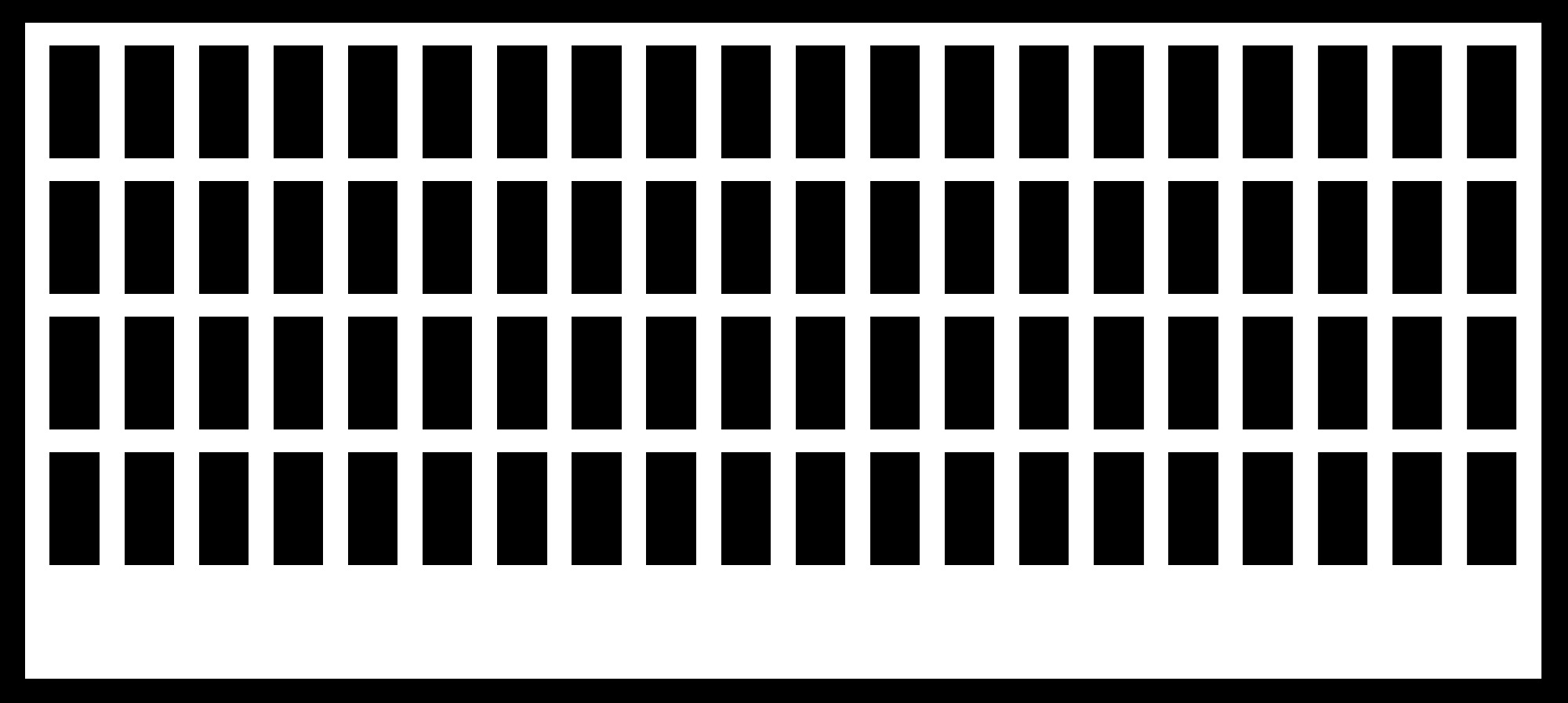
The comparison replicates the two scenarios proposed in [45]: the first one with a single room and fixed obstacles; the second one with 4 connected rooms. In both cases, the number of robots is varied to evaluate the collision-avoidance capabilities and the time consumption in finding a solution. In addition, a third scenario is proposed with a warehouse facility extracted from [41].

Figure 6 shows the first experimental scenario: a single 10 × 30 tiles room with a pattern of fixed obstacles similar to those presented in [49] but with a higher complexity. For this scenario, the number of robots varies from 3 to 15. Besides, Fig. 7 shows the second scenario, with four 10 × 30 tiles rooms connected 2-by-2 by means of 4 tiles long corridors. The rooms are free of obstacles and the robots are randomly located on each room. The goals for each robot are placed in a different room to force the robots to go through corridors. Again, the number of robots varies from 12 -3 robots per room- to 24 (6 robots per room). Finally, Fig. 8 depicts a warehouse scenario proposed in [41], where corridors are for one robot at a time with the exception of the lower area, where the picking stations are placed and up to three robots can pass over it.

Figure 6.

Graphical representation of scenery 1 used on experimentation.

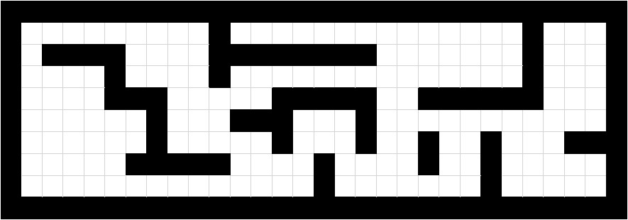
Figure 7.

Graphical representation of scenery 2 used on experimentation.

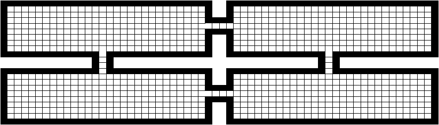
Figure 8.

Graphical representation of scenery 3 used on experimentation.

To compare the effectiveness of the solutions we incorporate the standard measurements [26]: i) the maximum distance travelled by any single-robot, and ii) the aggregated total distance. The total path-planning time for the MPP algorithms will be registered as well. Up to 10 runs of each algorithm and scenario will be run in order to estimate the statistics of the performances. During the experimentation, the parameters in the Table 1 were used.

4.Results and discussions

Figure 9.

Comparative graphs of the evolution of the execution time concerning the number of robots for each method. Scenario 1, 2 and 3 are shown at the upper, central and lower part, respectively. No results for M* are included for scenario 3 because its runtime for 10 robots’ is far too large.

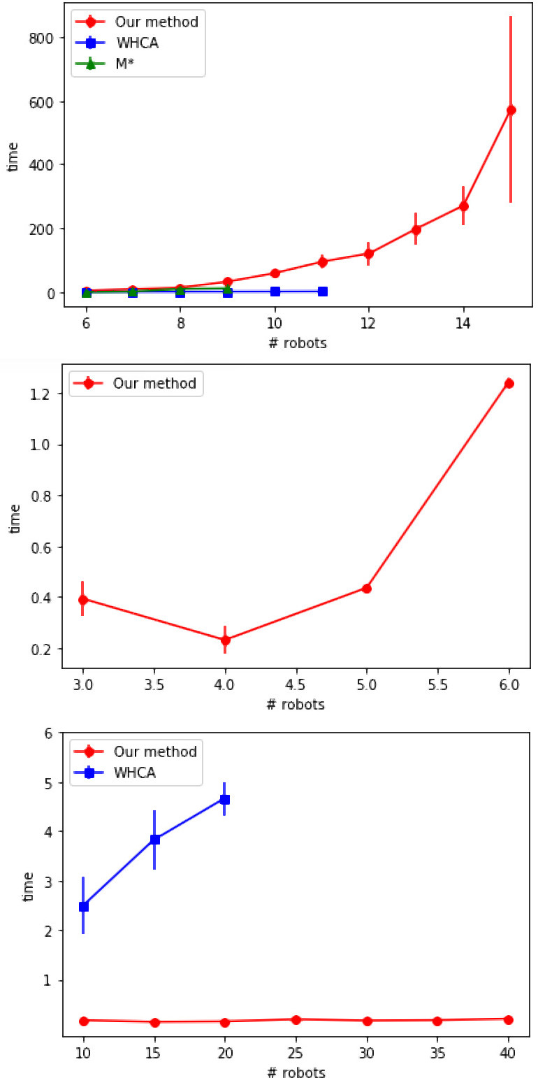
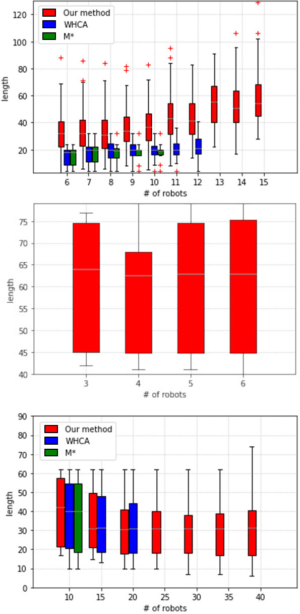
Figure 10.

Comparative graphs of the length of the paths concerning the number of robots for each method. Scenario 1, 2 and 3 are depicted at the upper, central and lower parts.

As mentioned before, two well-known metrics have been used: the execution time and the path length. Table 2 shows the numerical values obtained for the execution time metric, with gray cells for those methods that were not able to find a suitable solution for the corresponding scenario and number of robots. Interestingly, for scenario 2 our method was the single one that coped with the task satisfactorily.

Figure 9 graphically represents the execution cost of each method according to the scenario and the number of robots including the variance in the metric; as long as only our method found solutions for the second scenario and Table 2 includes the standard deviation, the corresponding figure is omitted. Probably, these results are due to the lack of heuristic search in the other methods as long as they are based on graph search. Interestingly, even though our method has a longer computational time in the first scenario, it can also obtain collision-free routes for a larger number of robots.

Figure 11.

Differences in the behaviour for the first scenario between the research in [45] and our research. In the upper part, the paths obtained using [45]; and the lower part, the paths obtained using our proposal.

Figure 12.

Differences in the behaviour for the first scenario between the research in [45] and our research. In the upper part, the paths obtained using [45]; and the lower part, the paths obtained using our proposal.

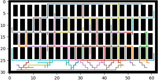
Figure 13.

Example of the routes in the third scenario.

No comparison can be made for the second scenario because only our method found solutions for the considered number of robots. It is clear that restricting the passages between rooms with very narrow corridors made the scenario so complex that only our proposal was able to find solutions.

For the third scenario, which is the most reliable representation of a warehouse environment, our method has the shortest execution time. The proposal in [45] was directly dismissed due to its poor performance in the previous scenarios. M* only found solutions for the smallest number of robots while WHCA proposed solutions for some number of robots, but in those cases the computation time was higher than our proposal. As for scenario 2, the problem of very restricted passageways seems to burden the M* and the WHCA.

The second used metric, the length of the paths, is included in Fig. 10 and Table 3. Figure 10 depicts the boxplots of the length of the paths from the different runs of the methods, while Table 3 includes i) the length of the longest path and ii) the sum of the lengths of all the paths of a solution. The same behaviour observed for the calculation time in the three scenarios is also present for this metric. In case of the first scenario, the lengths obtained with M* or WHCA were shorter than those obtained with our method, while the aggregated length among all the robots were comparable among all of them.

Several differences can be seen when analysing and comparing the routes proposed in [45] and those obtained in this research: in our method, keeping the collision-free A* paths forces the colliding robots to explore different alternatives and to make a better use of the available space. This can be clearly seen in Fig. 11 and Fig. 12; these figures plots the path generated for each robot using the two methods: the former corresponds with the first scenario and 10 robots, the latter with the second scenario and 3 robots per room. In the first scenario, the variety in the routes introduced by our approach is the one responsible of finding solutions where other proposals fail; however, exploring the domain has a cost in computation time. For the second scenario, the main difference is that the HALT operator reduces the collisions without further exploration of the space.

5.Conclusions

This study proposes a co-evolutionary algorithm with several improvements to solve the multi-robot path planning with collision avoidance, outperforming our previous research in [45]. The enhancements include i) keeping the collision-free robots’ A* routes, only evolving routes for the colliding robots, ii) reducing the search space by restricting the mutation points, and iii) tuning the probabilities of the movements to be considered in the mutation operator.

To evaluate this proposal, an experimentation in three different scenarios is proposed comparing our approach against two state-of-the-art methods -M* and WHCA- and also our previous research [45]. The obtained results show that our method is capable of finding solutions where the other three methods fail; however, this has a cost in computational time. The quality of the solutions in terms of length are comparable for scenarios such as warehouses.

Future research includes using different metaheuristics for optimization to reduce the computational time, which implies adapting them to the co-evolutionary process. Moreover, the solution space can be reduced by fixing some colliding robots -without collisions between them- and only finding routes for the remaining colliding robots. This can be solved using a sort of integer optimization to promote the A* alternatives. Considering multi-objective techniques to evaluate each route with the different metrics is still pending. These developments must also consider newly proposed learning algorithms, such as Neural Dynamic Classification algorithm [50], Dynamic Ensemble Learning Algorithm [51], and Finite Element Machine for fast learning [52]; these techniques can be used in the improvement of the metaheuristic design.

References

[1] | Mathew N, Smith SL, Waslander SL. Planning Paths for Package Delivery in Heterogeneous Multirobot Teams. IEEE Transactions on Automation Science and Engineering. (2015) ; 12: (4): 1298-1308. |
[2] | Tan Q, Denojean-Mairet M, Wang H, Zhang X, Pivot FC, Treu R. Toward a telepresence robot empowered smart lab. Smart Learning Environments. (2019) May; 6: (1): 5. |
[3] | Solak S, Yakut Ö, Dogru Bolat E. Design and Implementation of Web-Based Virtual Mobile Robot Laboratory for Engineering Education. Symmetry. (2020) ; 12: (6). |
[4] | Huang D, Jiang H, Yu Z, Kang C, Hu C. Leader-following Cluster Consensus in Multi-agent Systems with Intermittence. International Journal of Control, Automation and Systems. (2018) Apr; 16: (2): 437-451. |
[5] | Kumar NV, Kumar CS. Development of collision free path planning algorithm for warehouse mobile robot. Procedia Computer Science. (2018) ; 133: : 456-463. International Conference on Robotics and Smart Manufacturing (RoSMa2018). |
[6] | Stump E, Michael N. Multi-robot persistent surveillance planning as a Vehicle Routing Problem. In: 2011 IEEE International Conference on Automation Science and Engineering; (2011) . pp. 569-575. |
[7] | Shen H, Pan L, Qian J. Research on large-scale additive manufacturing based on multi-robot collaboration technology. Additive Manufacturing. (2019) ; 30: : 100906. |
[8] | Tisdale J, Kim Z, Hedrick JK. Autonomous UAV path planning and estimation. IEEE Robotics Automation Magazine. (2009) ; 16: (2):35-42. |
[9] | Chen X, Zhou B. A heuristics pulse algorithm with relaxation pruning strategy for resources re-initialized UAV path planing. Journal of Intelligent & Fuzzy Systems. (2021) ; 41: ((2)): 3541-3553. |
[10] | Liu R, Liang J, Alkhambashi M. Research on breakthrough and innovation of UAV mission planning method based on cloud computing-based reinforcement learning algorithm. Journal of Intelligent & Fuzzy Systems. (2019) ; 37: (3): 3285–3292. |
[11] | Yu J, LaValle S. Structure and Intractability of Optimal Multi-Robot Path Planning on Graphs. In: Proceedings of the AAAI Conference on Artificial Intelligence. vol. 27: ; (2013) . pp. 1443-1449. |
[12] | Stern R, Sturtevant N, Felner A, Koenig S, Ma H, Walker T, et al. Multi-Agent Pathfinding: Definitions, Variants, and Benchmarks. In: Proceedings of the Twelfth International Symposium on Combinatorial Search (SoCS 2019); (2019) . pp. 151-158. |
[13] | Surynek P. An Optimization Variant of Multi-Robot Path Planning Is Intractable. Proceedings of the AAAI Conference on Artificial Intelligence. (2010) Jul; 24: (1): 1261-1263. Available from: https://ojs.aaai.org/index.php/AAAI/article/view/7767. |
[14] | Hart PE, Nilsson NJ, Raphael B. A Formal Basis for the Heuristic Determination of Minimum Cost Paths. IEEE Transactions on Systems Science and Cybernetics. (1968) ; 4: (2):100–107. |
[15] | Silver D. Cooperative Pathfinding. In: Proceedings of the First AAAI Conference on Artificial Intelligence and Interactive Digital Entertainment (AIIDE’05); (2005) . pp. 117-122. Available from: https://www.aaai.org/Papers/AIIDE/2005/AIIDE05-020.pdf. |
[16] | Koenig S, Likhachev M. Fast replanning for navigation in unknown terrain. IEEE Transactions on Robotics. (2005) ; 21: (3): 354-363. |
[17] | Ferguson D, Stentz A. Using interpolation to improve path planning: The Field D* algorithm. Journal of Field Robotics. (2006) ; 23: (2): 79-101. Available from: https://onlinelibrary.wiley.com/doi/abs/10.1002/rob.20109. |
[18] | Daniel K, Nash A, Koenig S, Felner A. Theta*: Any-Angle Path Planning on Grids. Journal of Artificial Intelligence Research. (2010) Oct; 39: : 533-579. |
[19] | Wagner G, Choset H. M*: A complete multirobot path planning algorithm with performance bounds. In: 2011 IEEE/RSJ International Conference on Intelligent Robots and Systems; (2011) . pp. 3260-3267. |
[20] | Wagner G, Choset H. Subdimensional expansion for multirobot path planning. Artificial Intelligence. (2015) ; 219: :1-24. |
[21] | Standley TS. Finding Optimal Solutions to Cooperative Pathfinding Problems. In: Proceedings of the Twenty-Fourth AAAI Conference on Artificial Intelligences; (2010) . pp. 173-178. |
[22] | Standley TS, Korf RE. Complete Algorithms for Cooperative Pathfinding Problems. In: Proceedings of the Twenty-Second International Joint Conference on Artificial Intelligence; (2011) . pp. 668-673. |
[23] | Wahab MNA, Nefti-Meziani S, Atyabi A. A comparative review on mobile robot path planning: Classical or meta-heuristic methods? Annual Reviews in Control. (2020) ; 50: : 233-252. |
[24] | Setiawan YD, Pratama PS, Jeong SK, Duy VH, Kim SB. Experimental Comparison of A* and D* Lite Path Planning Algorithms for Differential Drive Automated Guided Vehicle. In: Zelinka I, Duy VH, Cha J, editors. AETA 2013: Recent Advances in Electrical Engineering and Related Sciences. Berlin, Heidelberg: Springer Berlin Heidelberg; (2014) . pp. 555-564. |
[25] | Lin S, Liu A, Wang J, Kong X. A Review of Path-Planning Approaches for Multiple Mobile Robots. Machines. (2022) ; 10: (9). |
[26] | Yu J, LaValle SM. Optimal Multirobot Path Planning on Graphs: Complete Algorithms and Effective Heuristics. IEEE Transactions on Robotics. (2016) ; 32: (5): 1163-1177. |
[27] | Sharon G, Stern R, Felner A, Sturtevant NR. Conflict-based search for optimal multi-agent pathfinding. Artificial Intelligence. (2015) ; 219: : 40-66. |
[28] | Zheng Y, Luo Q, Wang H, Wang C, Chen X. Path planning of mobile robot based on adaptive ant colony algorithm. Journal of Intelligent & Fuzzy Systems. (2020) ; 39: (4): 5329-5338. |
[29] | Gul F, Rahiman W, Alhady SSN, Ali A, Mir I, Jalil A. Meta-heuristic approach for solving multi-objective path planning for autonomous guided robot using PSO–GWO optimization algorithm with evolutionary programming. Journal of Ambient Intelligence and Humanize Computing. (2021) ; 12: : 7873-7890. |
[30] | Lacroix P, Polotski V, Cohen P. Decentralized Control of Cooperative Multi-robot Systems. Integrated Computer-Aided Engineering. (1999) ; 6: (4): 259-274. |
[31] | Dewangan RK, Shukla A, Godfrey WW. A solution for priority-based multi-robot path planning problem with obstacles using ant lion optimization. Modern Physics Letters B. (2020) ; 34: (13): 2050137. |
[32] | Chakraborty J, Konar A, Jain LC, Chakraborty UK. Cooperative multi-robot path planning using differential evolution. Journal of Intelligent & Fuzzy Systems. (2009) ; 20: (1-2): 13-27. |
[33] | Das PK, Behera HS, Das S, Tripathy HK, Panigrahi BK, Pradhan SK. A hybrid improved PSO-DV algorithm for multi-robot path planning in a clutter environment. Neurocomputing. (2016) ; 207: : 735-753. |
[34] | Das PK, Behera HS, Panigrahi BK. A hybridization of an improved particle swarm optimization and gravitational search algorithm for multi-robot path planning. Swarm and Evolutionary Computation. (2016) ; 28: : 14-28. |
[35] | Nazarahari M, Khanmirza E, Doostie S. Multi-objective multi-robot path planning in continuous environment using an enhanced genetic algorithm. Expert Systems with Applications. (2019) ; 115: : 106-120. |
[36] | Zhao T, Li H, Dian S. Multi-robot path planning based on improved artificial potential field and fuzzy inference system. Journal of Intelligent & Fuzzy Systems. (2020) ; 39: (5): 7621-7637. |
[37] | Kiadi M, Tan Q, Villar JR. Optimized Path Planning in Reinforcement Learning by Backtracking. Current Trends in Computer Sciences & Applications. (2019) ; 1: (4): 80-90. |
[38] | Bae H, Kim G, Kim J, Qian D, Lee S. Multi-Robot Path Planning Method Using Reinforcement Learning. Applied Sciences. (2019) ; 9: (15). Available from: https://www.mdpi.com/2076-3417/9/15/3057. |
[39] | Han SD, Yu J. Effective Heuristics for Multi-Robot Path Planning in Warehouse Environments. In: 2019 International Symposium on Multi-Robot and Multi-Agent Systems (MRS); (2019) . pp. 10-12. |
[40] | Chen X, Li Y, Liu L. A Coordinated Path Planning Algorithm for Multi-Robot in Intelligent Warehouse. In: 2019 IEEE International Conference on Robotics and Biomimetics (ROBIO); (2019) . pp. 2945-2950. |
[41] | Mei Y, Li S, Chen C, Han A. A Multi-robot Task Allocation and Path Planning Method for Warehouse System. In: 2021 40th Chinese Control Conference (CCC); (2021) . pp. 1911-1916. |
[42] | Han SD, Yu J. DDM: Fast Near-Optimal Multi-Robot Path Planning Using Diversified-Path and Optimal Sub-Problem Solution Database Heuristics. IEEE Robotics and Automation Letters. (2020) ; 5: (2): 1350-1357. |
[43] | Digani V, Sabattini L, Secchi C, Fantuzzi C. Ensemble Coordination Approach in Multi-AGV Systems Applied to Industrial Warehouses. IEEE Transactions on Automation Science and Engineering. (2015) ; 12: (3): 922-934. |
[44] | Liu Z, Wang H, Wei H, Liu M, Liu YH. Prediction, Planning, and Coordination of Thousand-Warehousing-Robot Networks With Motion and Communication Uncertainties. IEEE Transactions on Automation Science and Engineering. (2021) ; 18: (4): 1705-1717. |
[45] | Kiadi M, García E, Villar JR, Tan Q. A*-Based Co-Evolutionary Approach for Multi-Robot Path Planning with Collision Avoidance. Cybernetics and Systems. (2022) ; 0: (0): 1-16. |
[46] | Kociecki M, Adeli H. Shape optimization of free-form steel space-frame roof structures with complex geometries using evolutionary computing. Engineering Applications of Artificial Intelligence. (2015) ; 38: : 168-182. Available from: https://www.sciencedirect.com/science/article/pii/S0952197614002528. |
[47] | Oh BK, Kim KJ, Kim Y, Park HS, Adeli H. Evolutionary learning based sustainable strain sensing model for structural health monitoring of high-rise buildings. Applied Soft Computing. (2017) ; 58: : 576-585. Available from: https://www.sciencedirect.com/science/article/pii/S1568494617302922. |
[48] | Siddique N, Adeli H. Computational Intelligence – Synergies of Fuzzy Logic, Neural Networks and Evolutionary Computing. Wiley; (2013) . |
[49] | Qu H, Xing K, Alexander T. An improved genetic algorithm with coevolutionary strategy for global path planning of multiple mobile robots. Neurocomputing. (2013) ; 120: (0): 509-517. |
[50] | Rafiei MH, Adeli H. A New Neural Dynamic Classification Algorithm. IEEE Transactions on Neural Networks and Learning Systems. (2017) ; 28: (12): 3074-3083. |
[51] | Alam KMR, Siddique N, Adeli H. A Dynamic Ensemble Learning Algorithm for Neural Networks. Neural Computing and Applications. (2020) ; 32: (10): 8675-8680. |
[52] | Pereira DR, Piteri MA, Souza AN, Papa J, Adeli H. FEMa: A Finite Element Machine for Fast Learning. Neural Computing and Applications. (2020) ; 32: (10): 6393-6404. |