
A hybrid approach for improving the flexibility of production scheduling in flat steel industry
Abstract
Nowadays the steel market is becoming ever more competitive for European steelworks, especially as far as flat steel products are concerned. As such competition determines the price products, profit can be increased only by lowering production and commercial costs. Production yield can be significantly increased through an appropriate scheduling of the semi-manufactured products among the available sub-processes, to ensure that customers’ orders are timely completed, resources are optimally exploited, and delays are minimized. Therefore, an ever-increasing attention is paid toward production optimization through efficient scheduling strategies in the scientific and industrial communities. This paper proposes a hybrid approach to improve the flexibility of production scheduling in steelworks producing flat steel products. Such approach combines three methods holding different scopes and modelling different aspects: an auction-based multi-agent system is applied to face production uncertainties, multi-objective mixed-integer linear programming is used for global optimal scheduling of resources under steady conditions, while a continuous flow model copes with long-term production scheduling. According to the obtained simulation results, the integration and combination of these three approaches allow scheduling production in a flexible way by providing the capability to adapt to different production conditions.

1.Introduction
Nowadays the steel sector is dominated by a limited number of monopoly companies, which are often competing to preserve and possibly increase their shares on national and international markets. The product price is, therefore, determined by such competition, and profits can be increased mostly by reducing production and commercial costs. Companies that do not show to be flexible enough to update their strategies and their organizational processes, are automatically exposed to the risk of competitiveness loss. On the other hand, the steel sector is also facing the challenge of digitalization [1, 2], which opens new possibilities for implementing advanced approaches, including ones based on Artificial Intelligence (AI), in any aspects of production management and control. Digitalization also offers new opportunities and tools to increase productivity as an integral part of its socio-economic and environmental sustainability [3].
A feasible way to increase productivity in any company consists in creating a proper and optimized scheduling for components on available machines so that each order is completed on time, by maximizing resources use and minimizing the average production time.
Most scheduling problems are Non-deterministic Polynomial-Time Hard (NP-hard) [4, 5], i.e. the computational times of all known solving algorithms exponentially increase with problem size. Therefore, affordable procedures to find an optimal solution are not available. Production scheduling in the steel industry is recognized as one of the most difficult and complex industrial scheduling problems [6]. It involves several production steps, each of which needs multiple resources, such as materials, machineries, transport systems (e.g. cranes, forklifts), and needs to fulfil critical production constraints. Furthermore, the production process is often affected by unforeseen events, such as breakdowns and order cancellations, which can compromise the initial scheduling plan. Two main approaches are usually adopted to deal with production scheduling issues, namely deterministic and dynamic scheduling.
Classical deterministic approaches dominated the manufacturing scene for a long time and are still used. According to these approaches, all the parameters of the systems, such as number of jobs and machines processing time, are known in advance. Literature provides some interesting examples of deterministic scheduling useful for the steel sector [7, 8]. For instance, in [9] the Hot Strip Mill (HSM) production scheduling problem is formulated as a Prize Collecting Traveling Salesman Problem (PCTSP) model and solved through a Tabu Search (TS) approach. In [10] the production scheduling problem in a Cold Rolling Mill (CRM) is formulated in two parts, a coilmerging optimization and a batch planning model. The former problem is solved through a Discrete Differential Evolution (DDE) approach, while the latter one is faced through a hybrid heuristic approach. A scheduling approach for continuous galvanizing lines based on TS is presented in [11], while [12] discusses two hybrid strategies based on heuristic and metaheuristic methods facing the HSM scheduling. Multi-objective approaches have been also taken into account [13, 14]. However, all these approaches are unsuitable to cope with unforeseen events, such as breakdowns, special maintenance operations or delays in the arrival of raw materials, which can affect the schedule, by preventing fulfilment of the targeted goals.
![RAS cold rolling process scheme [32].](https://content.iospress.com:443/media/ica/2022/29-4/ica-29-4-ica220685/ica-29-ica220685-g001.jpg)
On the other hand, the problem of scheduling in presence of unforeseen events is addressed through dynamic scheduling strategies [15], and three main approaches are generally applied [16, 17], i.e. reactive, proactive and hybrid scheduling. In this context, [18, 19] propose a reactive scheduling approach based on Multi-Agent Systems (MASs) to solve the problem of integrated dynamic scheduling of continuous caster and HSM, although MASs have been applied in different cases [20, 21]. A reactive scheduling approach based on brokers in MASs for the dynamic resource allocation of a Cold Rolling (CR) process is presented in [22]. A reactive approach covering the whole production chain from primary steelmaking to CRM is presented in [23]. The re-scheduling problem is formulated as a Mixed-Integer Programming (MIP) model considering the original objective, the deviation from the initial scheduling and the equilibrium of production capacity, which is solved through a DDE algorithm. Further examples of reactive scheduling approaches can be found in [24, 25, 26, 27], which exploit different heuristics and metaheuristics techniques [13]. In [28] a proactive scheduling of coils at the CRM through a robust optimization problem solved by Particle Swarm Optimization (PSO) is promoted, while in [29] an ant-based agent system is presented to deal with asymmetric costs in scheduling. In [30] a proactive planning system is proposed, which optimizes the routing of steel coils among different processing lines by applying a multi-objective evolutionary algorithm, the Strength Pareto Evolutionary Algorithm 2 (SPEA2), to satisfy as set of Key Performance Indices (KPIs) defined on the basis of customer orders and production constraints. Another proactive scheduling for steel plates production is presented in [31], where Bayesian network models forecast the probability distributions of production loads and production times.
The reported literature review shows that production scheduling is mainly covered by deterministic, reactive and proactive approaches, while hybrid approaches are still rarely applied. Deterministic approaches assume a static environment with a fixed number of tasks to accomplish, deterministic processing times, machines continuously available and no unexpected events that would influence task processing when the schedule is executed. Proactive scheduling is designed to anticipate uncertainties and to reduce their impact on production schedules. Reactive scheduling is mainly used when preventing uncertainties is not possible due to lack of sufficient information, and fast actions must be made to readapt the scheduling whenever an anomalous event appears. Finally, hybrid scheduling exploits both proactive methods to define the preventive schedule and reactive approaches to deal with uncertainties not covered by the proactive initial phase. Each approach copes with different degrees of uncertainty. Hybrid approaches try to cover the range of uncertainty as much as possible, but the complexity of such approaches is much higher than single approaches.
This paper presents a hybrid approach for improving the flexibility of production scheduling in flat steel production, which combines and integrates different strategies: a Multi-Objective Mixed-Integer Linear Programming (MOMILP)-based approach supports global optimal resources scheduling under steady conditions, an auction-based MAS is used to deal with uncertainties of the production, and a Continuous Flow Model (CFM) approach faces long-term production scheduling. Each method has a distinct scope and different modelling aspects which allow coping with dynamic aspects of the production. All these aspects may be tackled by a hybrid approach taking the advantage of mixing different strategies to deal with uncertainties while taking into account the achievement of the company’s objectives. Compared to previous literature works on the same subject, the proposed combined approach allows scheduling production in a flexible way and is capable to adapt to different production conditions, by merging the benefits of the single approaches while overcoming their drawbacks. Therefore, it allows increasing production efficiency with cost and resource savings, achieving higher product quality and maximizing plant performance.
Table 1
Notation used for the formulation of the scheduling problem and for the optimization methods
| Variable | Description |
|---|---|
|
| Machine environment |
|
| Job characteristic and constraints |
|
| Objective function |
|
| Set of |
|
| Amount of product |
|
| Processing rate of product |
|
| Proportion of product |
|
| Demand of product |
|
| Upper limit of production on machine |
| Lower and upper limit of storage | |
|
| Production quantity cost function related to demand of product |
|
| Cost related to demand of product |
|
| Production cost function related to product |
|
| Cost related to production of product |
|
| Usage cost function related to product |
|
| Cost related to usage of machine |
|
| Storage cost function related to product |
| Penalty costs related to storage of product | |
|
| Change cost function related to product |
|
| Cost related to change of product |
|
| Objective functions |
|
| Vector of variables |
|
| Vector of costs associated to problem |
|
| Matrices for inequality and equality constraints |
| Lower and upper bounds of | |
|
| Set of jobs |
|
| Set of machines |
|
| Set of production stages |
|
| Processing time of job |
|
| Setup time of machine |
|
| Minimum process-related idle time that job |
|
| Binary variable, true when job |
| Binary variable, true when job | |
|
| Weight of job |
|
| Total weight of jobs waiting to be processed at stage |
| Minimum and maximum capacity of warehouse at stage | |
|
| Binary variable, true when job |
| Binary variable, true when job | |
| Starting time of job | |
|
| Finishing time of job |
| Binary variable, true when job | |
|
| Binary variable, true when job |
|
| Set of machines at stage |
|
| Waiting time of job |
|
| Problem constant |
|
| Binary variable, true when job |
|
| Makespan |
|
| Upper bound of makespan |
|
| Throughput cost function |
|
| Overall completion time cost function |
The paper is organized as follows. Section 2 briefly describes the real industrial use case and formalises the scheduling problem. In Section 3 the proposed hybrid approach for flexible production scheduling is presented and in Section 4 a detailed description of each method is reported. Numerical simulation results are presented and discussed in Section 5. Finally, Section 6 proposes some concluding remarks and hints for future work.
2.Use case description
Steel is cold rolled to produce flat products such as deep-drawing sheet and packaging steel. The most widespread process is the strip CR, which exploits hot rolled strips as raw material and outputs flat products in different shapes. In particular, the industrial process addressed in this work is the CR process of Rasselstein (RAS), a company located in Andernach, Germany, which is schematically depicted in Fig. 1.
Figure 2.
Machine environment scheme.
The first step of the production chain is the pickling process, where the scale that has formed on the surface of the hot rolled strips is removed using diluted sulfuric acid. Afterwards, semi-finished products are cold rolled by five- or six-stand tandem CR mills. In this process, the steel strip thickness is reduced by approximately 90% by high pressure in the stands. A palm oil/water mixture is used for cooling the strip. CR produces a smoother surface with higher dimensional accuracy and, due to the work hardening effect, greater strength as well. In order to eliminate work hardening after CR, heat treatment by annealing, e.g. batch-based or continuous-based, is frequently applied. A degreasing process is usually carried out before annealing, to remove substances from the surface of cold rolled strips such as mineral or vegetable oils coming from mechanical processing and cleaning. After annealing and temper rolling, two types of coating processes are carried out, i.e. tinning and chromium plating, which provide corrosion resistance. This production step is then followed by other treatments, such as film laminating and lacquering, slitting, cutting, recoiling, etc.
2.1Problem formulation
A scheduling problem consists of assigning jobs to machines at each stage (global routing) and sequencing the jobs assigned to the same machine (local sequencing) so that some optimality criteria are minimized. Most real-life scheduling problems are essentially more complex than those considered in scheduling theory. Here, the production process at RAS is mapped through a framework and notation commonly used in production planning [33] and summarized in Table 1. According to this notation, classes of scheduling problems are specified by a classification triplet
• the
• the
• the
In the present work, the scheduling problem from pickling to coating stages is covered. The production system is composed of multiple production stages, and there are parallel machines for all of the stages except the first stage (i.e. pickling). Each machine in parallel has its own properties. Therefore, the whole production is a generalization of the flow shop with different production stages and unrelated machines in parallel, i.e. flexible flow shop or hybrid flow shop, described as follows:
(1)
where
A scheme of the considered machine environment is shown in Fig. 2. There are 1 pickling (P1), 2 CRs (CR1 and CR2), 5 degreasing (D1, D2, D3, D4 and D5), 5 annealing (2 batch BA1 and BA2, 3 continuous CA1, CA2 and CA3), 3 temper rolling (TR1, TR2 and TR3) and 5 coating (CO1, CO2, CO3, CO4 and CO5) machines located at stages 1 to 6. For the continuous annealing lines, the degreasing operation is integrated in the plant, thus, for these lines the degreasing stage was added to the machine environment as (D3-D5). However, there is a strict production path from D3-D5 to CA1-CA3, such as shown in Fig. 2. The lines at each stage are also characterized by different speed values and functionalities, processing quantities and qualities and setup times. Intermediate buffers are used for supporting continuous production, where output products of the previous process stage are stored and serve as inputs for the next processing step. Furthermore, the stocks of semi-finished products have different capacities.
To classify the
• All facilities except BA1 and BA2 can process jobs individually at a given time, which means that for BA1 and BA2,
• Since CR is a sequential production, process and jobs must be completed before another job is allowed to start; thus, the precedence constraint
• Machines at each stage have different criteria and their inputs and outputs may be different. Usually, planners take only some special machines into account to produce specific products. Hence for such a job, the constraint
• At all stages, preemptions are not allowed.
• Machines may not be continuously available, as breakdowns can occur, which may cause severe capacity losses; thus, the constraint
The objective to minimize, i.e. the
3.Hybrid approach for flexible production scheduling
Computer-aided Production Planning and Control (PPC) systems are used for the operational planning and control of product activities in an industrial plant [35]. Over the past decades, various concepts for production planning and control have emerged, although the hierarchical-sequential arrangement of PPC tasks clearly predominates [36]. An overview and comparison of 20 different PPC concepts is compiled by Meudt et al. [37].
While the pure commercial processes in the different industries do not significantly differ, the production cycles show their individual as well as partly unique characteristics and require special solutions in the PPC environment. Although specific solutions with a steel focus have been developed for individual selected PPC tasks, a holistic approach for the task of in-house production planning and control at the different planning levels is missing. Indeed, these characteristics can be found not just in steel industry but in other similar production industries such as paper or aluminium coil production, or wafer fabrication facilities in semi-conductor industry, where different factors may occur such as unexpected breakdowns, last minute order changes because of quality issues, stocking limitations for work in progress products or urgent orders requiring changes in production prioritization. Actually, Fig. 3 shows the average number of those events asking for continuous production replanning.
Figure 3.
Frequency distribution of rescheduling with causes over a period of one week. Average values derived from different flat steel facilities producing base material for several industries (cars, food packaging, etc.).
Figure 4.
Hybrid approach scheme.
The proposed hybrid scheduling approach addresses this issue. The scheme of the developed approach is depicted in Fig. 4, where, on the vertical axis, the planning horizon is reported, while the planning accuracy of each method is reported on the horizontal axis. This approach can be divided into three levels with different planning horizons as well as planning accuracies, which are described in more detail in the next subsections.
3.1Long-term planning
In industries with flexible flow production schemas, production programs are often compiled on the basis of order-less product structures and their quantity-related characteristics over a production period. These product structures comprise aggregations of finished materials with similar material flows within production. In these material flows, a high degree of branching can occur with increasing vertical integration and complexity, which is why the structures of semi-finished products also show a high planning relevance. This aspect is addressed by the long-term planning level (monthly basis) of the hybrid scheduling approach by taking into account the development of inventories and their structures per manufacturing level together with the defined planning limits. On this basis, rough feasibility studies of these order-less production programs can be carried out as well as capacity planning with the stored shift patterns from workforce scheduling. For fast and comprehensible results, the top of the pyramid with its CFM is applied. In this order-less approach for the long-term horizon, the planning problem is simplified to a reasonable level. Hence, a manufacturing system can be approximately represented by a time-continuous or time-discrete dynamic model. The development of a dynamic model of a manufacturing system requires the definition of state (inventory at each production stage) and control variables (production). Besides, the capacity constraints are also considered in this model. The formulated continuous scheduling problem is an optimal control problem with state constraints, and then this can be calculated in a rendering horizontal scheme [38]. Different production routes of the relevant product groups can be taken into account in this mass flow method. At this level, the user can exploit these options to plan capacities and coordinate the product portfolio to be produced (lowest planning accuracy of the three levels of the hybrid approach).
3.2Mid-term planning
After the release from sales department, the production program is filled with concrete orders, which serve as an order backlog for the mid-term planning level of the hybrid scheduling approach. Under static conditions and a higher level of details, valid order lots (group of orders in a defined sequence) are created per plant with orders from the pool in sequence planning, which also takes into account the steel-specific aspect of the development of the inventory structures as well as plant-related restrictions. This mid-term planning task is carried out by a MOMILP algorithm, whereby the planning targets are taken from long-term planning and extended by additional order-related objectives (e.g., minimization of delays). It provides a preliminary global optimal resource scheduling under static conditions, i.e., based on production orders and not considering unexpected events. MILP techniques are used to solve different types of industrial problems, including gas distribution [39], cutting and packing [40], energy and by-products management [41, 42], production planning [43] and scheduling [44]. Their importance lies in both their wide application and the availability of effective general-purpose techniques for finding nearly optimal solutions. However, the techniques require high computation time, which is a disadvantage that makes dynamic scheduling for continuous production difficult. To reduce the computation time, a complexity reduction of the optimization problem has been integrated. With this tool, the user can create plans regarding the routing and sequencing of released orders at medium level of planning accuracy.
3.3Short-term planning
Short-term planning at the shop-floor level relates to material pieces/coils allocated to the planned orders from the lots defined in mid-term planning. The high planning accuracy derived from this stage is further tightened by taking into account all relevant data in real-time. Due to the dynamic environment characterizing flat steel industry, this capability is essential for the required huge degree of flexibility. Therefore, this short-term planning task is realized through an auction-based MAS predestined for uncertain scheduling environments regarding resource availability, and is characterized by its responsiveness, flexibility and robustness. On a negotiation platform, different agents represent production facilities, the coils to be produced, and auxiliary agents. Thereby, coils can bid on different auction processes at each resource with an available virtual budget de-pending on their status. Concerning the lowest virtual costs, the utility maximization of each resource agent is balanced with the coil agent’s objective. This approach acts towards the user as an adviser and delivers robust reaction strategies based on real-time process data. Whereas global optimality conditions are taken into account at mid-term planning, the short-term approach focuses on considering advanced aspects depending on the current status of the manufacturing plants, such as regularity in the sequence of coils being processed, as an additional constraint to increase the quality of the operations.
Figure 5.
Hybrid approach scheme.

3.4Interaction among planning levels
The workflow showing the interaction among the methods follows a top-down strategy is shown in Fig. 5. The user controls the hybrid planning process at the long-term planning level and provides information on the current storage capacities, the selected production strategy, and planned downtimes to the CFM. Due to the simplified problem formulation, the CFM can provide a flow-optimized long-term planning with a planning horizon of 1–2 months. For each production facility this planning is provided as per-day production targets to the mid-term planning level (e.g., target amount of tons per material per day). According to these targets the MOMILP selects suitable orders from the order-book and produces an order-optimal target schedule for each production facility, which is provided to the coil-based MAS for execution. The MAS can provide flexible real-time schedules which can consider the current production state and react dynamically on incidents without the need for a full replanning.
The hybrid approach improves robustness and transparency of the production planning results considering a global production strategy. A detail description of each method is reported in the next section.
4.Applied methods for hybrid approach
4.1Continuous flow model approach
For long-term planning it is reasonable to simplify the formulation of the planning problem. Therefore, a manufacturing system can be represented approximately by a time continuous or time discrete dynamic model. Let us for instance consider a
Figure 6.
The following model applies to the first storage:
(2)
and to all others:
(3)
where
The objective function to be minimize is the following:
(4)
where
The production costs and other quality parameters per product
If more than one production route for a product is possible or if the full capacity of the machines is not necessary for the production, the use of a machine
The deviation from the pre-set storage level can be considered as
Furthermore, a frequent change between the products can be dampened or prevented by the following
4.2Multi-objective mixed-integer linear programming approach
The proposed approach is based on the lexicographic method [45], which is an a priori method, used when a preference exists among the objective functions, and a Pareto front is not needed because trade-off information is not required. Let
(5)
here
Furthermore, an iterative strategy that allows producing a scheduling of a selected number of jobs over a specific timeframe has been implemented. In this way, the algorithm is run iteratively with updated plant information. At each iteration a number of jobs is selected to be processed. A job is considered as a group of coils belonging to the same order, and this group is processed as a unique block from start to end of its production. Modelling jobs instead of single semi-finished products allows the mathematical optimization solver managing problem variables in an easier way, by avoiding computational overloading and long optimization times.
A detailed description of the mathematical formalization of the optimization problem follows. Some of its parts are based on the work of Hadera et al. [46].
4.2.1Sets and parameters
Let
In order to model jobs priorities, binary parameters
Each job
4.2.2Variables
To model the assignment of job
Binary variables
4.2.3Constraints and objective functions
The following equality and inequalities serve to model the constraints of the problem and mathematically define the variables. Exactly
(6)
where
The finishing time of job
(7)
The next equation defines the waiting time between stages as the difference between the starting time of stage
(8)
Waiting times between stages have restrictions: a job should wait at least its process-related idle time needed to be processed on the next stage:
(9)
where
The precedence relations are defined by the following equations, which express the fact that if
(10)
The following equation allows the precedence relation between two jobs being well defined: either
(11)
To model the strict production path from D1 and D2 to BA1 and BA2, and from D3, D4, and D5 to CA1, CA2 and CA3 the following set of constraints were considered:
(12)
(13)
(14)
(15)
(16)
(17)
(18)
To model the requirement of an order related to batch or continuous annealing the following set of constraints are considered:
(19)
(20)
The constraint to ensure priority of a job is modelled as follows:
(21)
A job can perform only stages that it has not yet performed. This is modelled by the constraint:
(22)
Moreover, a stage can be completed only if the previous stages have been completed, therefore:
(23)
The latest ending time for the scheduling must not be exceeded at any given moment, this is ensured by the equation:
(24)
where
The following constraints ensures that the weight stocked at a given warehouse lies within the limits at any moment:
(25)
(26)
Finally, the total weight of jobs (throughput) that undergo each production stage must be maximized: thus, the minimum of the following objective function is sought:
(27)
It is also possible to maximize only the total weight of jobs that complete the last production stage
(28)
Therefore, the overall completion time measured by the sum of the finishing times of all the jobs in all the stages is minimized.
Once the MILP algorithm has found a solution, the parameters are updated accordingly: parameters
In order to run the algorithm in an iterative way, the finishing times of jobs on a machine
4.3Auction-based multi-agent approach
While the MOMILP approach works at order level, the auction-based multi-agent scheduling system was selected as a convenient alternative to the local sequencing problem at coil level, providing enough feasibility and flexibility when uncertainty regarding resource availability is relevant.
For the short-term scheduling a negotiation platform is setup using the Extensible Messaging and Presence Protocol (XMPP), where different agents representing the relevant production plants and the coils being produced, as well as some auxiliary agents (logger, launcher and browser agents) exchange information in real time. The adopted architecture enables distributing negotiations, where the platform can be operated inside one container, virtual system or computer, while agents can operate at different systems connected through TCP protocol. In order to avoid inter-lock mechanisms an asynchronous dialog was implemented.
Figure 7.
Sequence diagram adopted by the continuous annealing agent in auction state.
Figure 7 shows the designed autonomous MAS and the implemented sequence diagram for an agent representing a continuous annealing plant, where some of the innovative components are introduced.
Several actors are involved in the system:
• Coil agent: it refers to each individual coil in production. It is equipped with the recommended routing as well as with operating characteristics and a virtual budget, allowing them to bid to the different auction processes at the different resources, according to their status.
• Resource agents: two types of Resource Agent are implemented: Transportation Agent and Warehouse Agent. The former moves coils from one location to another one, the latter provides information about availability to drop coils, has predefined capacity and admits or rejects reservation as function of current load and capacity.
• Plant agent: it is responsible to support the auction at any time. It books transportation to transport the coil to the resource, books warehouse space, checking in both cases for real-time availability. It negotiates with active Coil Agents searching to be processed and informs Log Agent of won bid in case of assigned processing to coil.
• Virtual agents: two types of Virtual Agent have been implemented, Log Agent and Browser Agent. The former traces communications and actions that are being taken in the system, the latter checks log registers and provides requested information to agents in the system (for instance Plant Agents ask for the current active coils).
Multi-optimization objectives are allowed, where an equilibrium among benefits for plants and for coils need to be found in an incremental way. The auction is a multistep system including counterbidding. The bidding also includes intelligence, as the Coil Agent can be aware of the averaged costs from previous auctions and it is sensitive to the urgency, depending on the deadline and the number of failed auctions already experienced, by using a rule-based approach. Additional complexity can be implemented by integrating inner logistics rules in the scoring process of Coil Agents bidding for available production slots throughout a subagent mechanism, where the Plant Agent is in charge of recruiting transport and warehouse resources for the operation before launching the auction itself (pre-auction phase), where different costs for inner logistics are considered. Dialog with plant and sub-agents is highlighted in blue colour in Fig. 7, where sequence diagram describes the communication flows in asynchronous way between the involved agents.
Initially the coils belong to specific orders where their production route is defined as a string sequence of plants separated by a ‘;’, accepting regular expression such as “P1;CR2;D[3-5];CA[1,3];TR[2-3];CO.*”. Coils belonging to the same order inherits the sequence, in such a way they know the targeted plants, so the agent representing the coil can apply when such plants offer an auction. Such approach also allows that if a coil fails in achieving the required quality thresholds, it can be reassigned to a different order, including a different route of targeted plants, by means of the launcher agent.
Figure 8.
Two stage process with two products.
On the side of the plant, after submitting invitation to coils present in the negotiation platform and collecting the submitted bids for those interested in the auction, a preliminary scoring approach is conducted and based on it, a counterbid is requested to such coils. When the counterbid is received, the final rank is produced and confirmation is requested to winner, with rotation in case of not agreement. When confirmed, resolution messages are sent to the not winning participants and auction becomes closed. Then, cycle starts again.
In the scoring process currently similarity to the actual operation parameters is used as fitness criteria, to get smooth transitions between coils in the production sequence. However, more advanced criteria can be easily implemented, such as estimated energy required during process among other aspects.
5.Results
5.1Case A: Long-term planning with prediction of material flow and storage level
In the first experiment, the long-term planning of a a two-step process (e.g. pickling and CR) as shown in Fig. 8 is performed. Two different products,
Figure 9.
The quality of the figure but also of other figures present in the paper have been reduced compared to the reviewed manuscript.
Table 2
Daily produced product quantity of
| Days | ||||
|---|---|---|---|---|
| 1 | 1000 | 800 | 1600 | 1400 |
| 2 | 1000 | 800 | 1000 | 800 |
| 3 | 1000 | 800 | 1000 | 800 |
| 4 | 1000 | 800 | 1000 | 800 |
| 5 | 1000 | 800 | 0 | 800 |
| 6 | 1000 | 800 | 0 | 800 |
| 7 | 0 | 800 | 0 | 800 |
| 8 | 0 | 800 | 0 | 800 |
| 9 | 3000 | 800 | 5000 | 800 |
| 10 | 1000 | 800 | 1000 | 800 |
| 11 | 1000 | 800 | 1000 | 800 |
| 12 | 1000 | 800 | 1000 | 800 |
| 13 | 1000 | 800 | 1000 | 800 |
| 14 | 1000 | 800 | 1000 | 800 |
| 15 | 1000 | 800 | 1000 | 800 |
| 16 | 1000 | 800 | 1000 | 800 |
| 17 | 1000 | 800 | 1000 | 800 |
| 18 | 0 | 800 | 0 | 800 |
| 19 | 0 | 800 | 0 | 800 |
| 20 | 0 | 800 | 0 | 800 |
| 21 | 0 | 800 | 0 | 800 |
| 22 | 3657 | 800 | 3657 | 800 |
| 23 | 2343 | 800 | 2343 | 800 |
| 24 | 1000 | 800 | 1000 | 800 |
| 25 | 1000 | 800 | 1000 | 800 |
| 26 | 1000 | 800 | 1000 | 800 |
| 27 | 1000 | 800 | 1000 | 800 |
| 28 | 1000 | 800 | 1000 | 800 |
| 29 | 1000 | 800 | 1000 | 800 |
| 30 | 1086 | 950 | 1136 | 842 |
The simulation is performed in MATLAB
5.2Case B: Mid-term planning for global scheduling with production targets
In the second experiment, the MOMILP-based approach is fed with production targets provided by the CFM. The objective is to provide the global scheduling of several jobs under static conditions aiming at satisfying quantities provided by the CFM with a 10% of tolerance.
The designed MOMILP-based approach is implemented through the PuLP library of Python programming language. The library allows modelling linear programming problems and is supported by different optimization solvers. In particular, the solver used for the simulation is GUROBI, which shows the best performances among the tested ones. Furthermore, Gantt charts are used for the graphical representations of the scheduling, which are built through Plotly (a library for Python based on the Dash framework).
In the simulation experiment, the global scheduling of 700 jobs each of which composed of 3 coils with a weight of 10 tons has to be accomplished in a daily timeframe. Jobs are selected according to their due date and are equally distributed among the production stages. Since a job can be batch or continuous annealed, its routing path is randomly selected by properly initializing the flags
Table 3
Initial stock of semi-finished products
| Stage | Stocks (%) |
|---|---|
| 1 | 63.9 |
| 2 | 19.4 |
| 3 | 25.0 |
| 4 | 13.3 |
| 5 | 36.1 |
| 6 | 19.4 |
Table 4
Planned stock limits of semi-finished products
| Max. (%) | Min. (%) | |
|---|---|---|
| Pickled material | 41.7 | 11.1 |
| Cold rolled material | 38.9 | 22.8 |
| Degreased material | 16.7 | 2.8 |
| Annealed material | 52.2 | 30.6 |
| Temper rolled material | 33.3 | 13.9 |
| Coating material | 66.7 | – |
Table 5
Optimization performances for each iteration (
| It. | ||||
|---|---|---|---|---|
| 1 | 0.0 | 5.1 | 69.6 | 300.5 |
| 2 | 8.9 | 300.3 | 30.2 | 300.1 |
| 3 | 0.0 | 5.8 | 14.6 | 300.5 |
| 4 | 0.0 | 6.0 | 10.8 | 300.3 |
| 5 | 0.0 | 1.7 | 9.8 | 301.0 |
The scheduling problem is solved in 5 iterations so that the solver can handle more jobs in the selected timeframe. For each iteration, 140 jobs are handled by the MILP algorithm. The time limit for the solver has been set to 5 minutes for each SOO sub-problem. The solution found by the optimizer is not far from being optimal, such as shown in Table 5. An average gap of 1.8% from the best bound for the first sub-problem (optimising
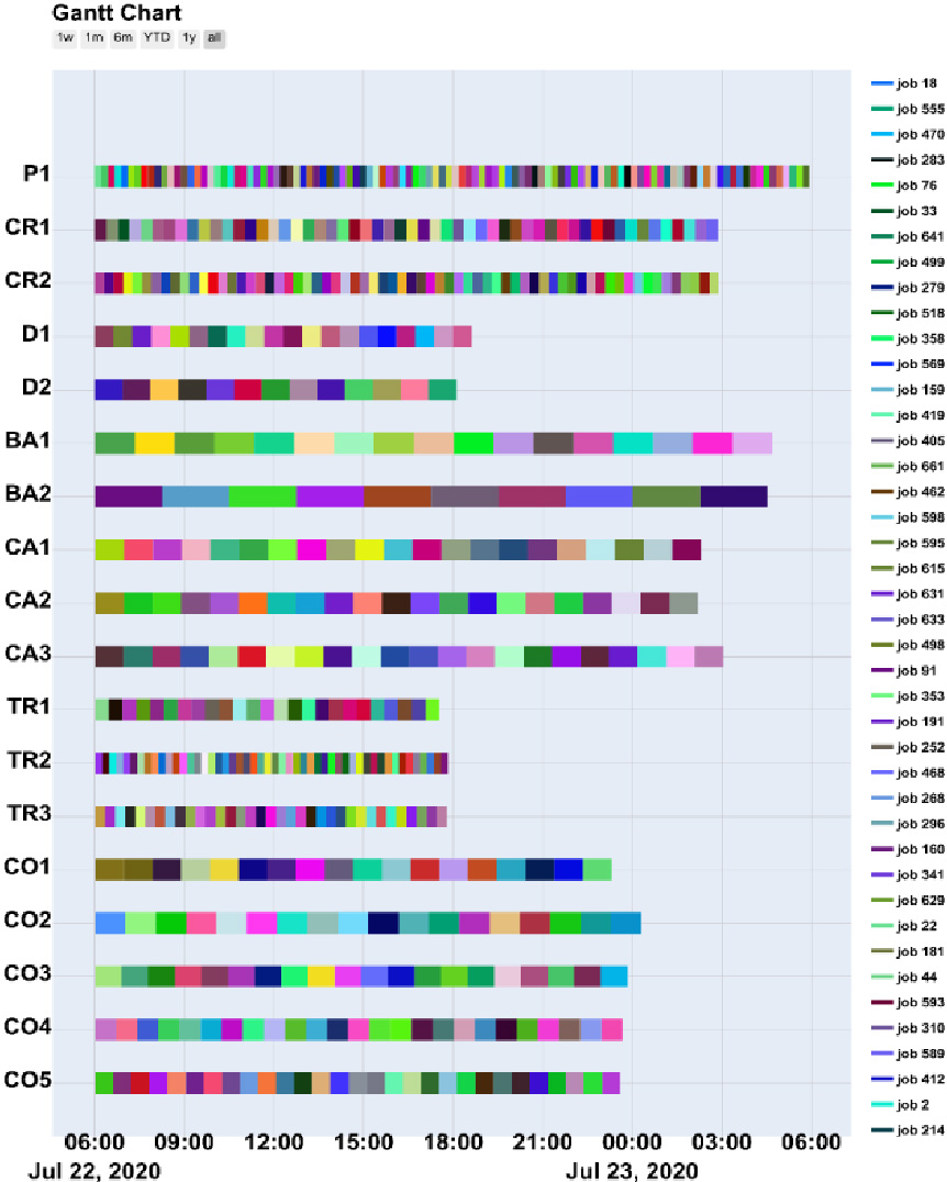
The Gantt chart of the simulation is shown in Fig. 10 (for the sake of clarity, the legend shows only few jobs although their number is far higher).
Table 6
Number of jobs completed at the end of the simulation for each iteration
| Stage | ||||||
|---|---|---|---|---|---|---|
| It. | 1 | 2 | 3 | 4 | 5 | 6 |
| 1 | 22 | 24 | 13 | 35 | 23 | 24 |
| 2 | 23 | 24 | 23 | 18 | 23 | 23 |
| 3 | 24 | 24 | 23 | 14 | 23 | 22 |
| 4 | 14 | 20 | 23 | 10 | 15 | 21 |
| 5 | 0 | 0 | 3 | 3 | 0 | 20 |
Figure 10.
Gantt chart of the scheduling provided by the MOMILP-based approach.
The total number of jobs completed at each stage as well as the weight distribution of stocks at end of the simulation and the production targets for each iteration are reported in Tables 6–8 respectively. The values reported in Table 7 comply with the limits provided in Table 4, as well as the optimized throughput at each production stage provided by the MOMILP satisfy the production targets of the CFM with the desired tolerance as reported in Table 8.
Table 7
Plant stocks (%) at the end of the simulation for each iteration
| Stage | ||||||
|---|---|---|---|---|---|---|
| It. | 1 | 2 | 3 | 4 | 5 | 6 |
| 1 | 60.2 | 19.1 | 26.8 | 9.7 | 38.1 | 19.3 |
| 2 | 56.4 | 18.9 | 27.0 | 10.5 | 37.3 | 19.3 |
| 3 | 52.4 | 18.9 | 27.2 | 12.0 | 35.8 | 19.4 |
| 4 | 50.1 | 17.9 | 26.7 | 14.2 | 34.9 | 18.4 |
| 5 | 50.1 | 17.9 | 26.2 | 14.2 | 35.4 | 15.1 |
Table 8
Production targets of CFM and MOMILP optimized throughput for each production stage
| Stage | Targets (tons) | Completed (tons) |
|---|---|---|
| 1 | 2270 | 2490 |
| 2 | 2520 | 2720 |
| 3 | 2330 | 2550 |
| 4 | 2190 | 2400 |
| 5 | 2310 | 2520 |
| 6 | 3300 | 3300 |
5.3Case C: Mid-term planning and short-term reaction for global scheduling and local sequencing
In the third experiment, a combination of the designed MOMILP-based approach and the auction-based MAS is implemented. The former approach provides the global scheduling of several jobs under static conditions. The outcome of this method is used by the MAS, which enables short-term local optimal decision-making process granting consideration for detailed production rules as per resource. For this second part of the experiment, only the coating stage of the CR use case described in Section 2 has been considered, because it is enough to show sensibility for production and breakdowns. The MAS system enables dynamic decision, while plant breakdown is represented by stopping the equivalent plant agent. This approach also reduces pressure over the technical decision makers when disruption happens, because the dynamic behaviour of MAS enables coil agents to participate in auctions raised by compatible plants still in operation because of the regular expression describing the targeted plants at every step.
5.3.1MOMILP-based simulation test
In the simulation experiment, the global scheduling of 700 jobs each of which composed of 3 coils with a weight of 10 tons has to be accomplished in a daily timeframe. Same considerations are drawn for jobs selection, initial stocked materials, machine average processing times, machine setup times, process-related idle times and stocks weight limits as reported in Case B.
Table 9
Optimization performances for each iteration (
| It. | ||||
|---|---|---|---|---|
| 1 | 0.0 | 5.1 | 69.6 | 300.4 |
| 2 | 8.9 | 300.3 | 30.2 | 300.1 |
| 3 | 0.0 | 5.4 | 14.6 | 300.5 |
| 4 | 0.0 | 5.8 | 9.7 | 300.5 |
| 5 | 11.4 | 300.3 | 9.7 | 300.1 |
The scheduling problem is solved in 5 iterations, and 140 jobs are handled by the MILP algorithm for each iteration. The time limit for the solver has been set to 5 minutes for each SOO sub-problem. The solution found by the optimizer is not far from being optimal, such as shown in Table 9. An average gap of 4.1% from the best bound for the first subproblem (optimising
Table 10
Number of jobs completed at the end of the simulation for each iteration
| Stage | ||||||
|---|---|---|---|---|---|---|
| It. | 1 | 2 | 3 | 4 | 5 | 6 |
| 1 | 22 | 24 | 13 | 35 | 23 | 24 |
| 2 | 23 | 24 | 23 | 18 | 23 | 23 |
| 3 | 24 | 24 | 23 | 14 | 23 | 22 |
| 4 | 25 | 24 | 23 | 10 | 23 | 21 |
| 5 | 14 | 24 | 15 | 14 | 18 | 20 |
The Gantt chart of the simulation results is shown in Fig. 11 (for the sake of clarity, the legend shows only few jobs although their number is far higher).
The total number of jobs completed at each stage as well as the weight distribution of stocks at the end of the simulation for each iteration are reported in Tables 10 and 11, respectively. The values reported in Table 11 comply with the limits provided in Table 4.
Table 11
Plant stocks (%) at the end of the simulation for each iteration
| Stage | ||||||
|---|---|---|---|---|---|---|
| It. | 1 | 2 | 3 | 4 | 5 | 6 |
| 1 | 60.2 | 19.1 | 26.8 | 9.7 | 38.1 | 19.3 |
| 2 | 56.4 | 18.9 | 27.0 | 10.5 | 37.3 | 19.3 |
| 3 | 52.4 | 18.9 | 27.2 | 12.0 | 35.8 | 19.4 |
| 4 | 48.2 | 19.1 | 27.3 | 14.2 | 33.6 | 19.8 |
| 5 | 45.9 | 17.4 | 28.8 | 14.3 | 32.9 | 19.4 |
Table 12
Structure of the order sequence obtained for coating plants
| OrderID | JobID | Plant | Storage | Sequence |
|---|---|---|---|---|
| 326596 | 140 | CO0[1-2] | K | 1 |
| 326597 | 120 | CO0[1-2] | K | 2 |
| 326598 | 126 | CO0[1-2] | K | 3 |
| 330151 | 130 | CO0[1-2] | K | 4 |
|
|
|
|
|
|
Figure 11.
Gantt chart of the scheduling provided by the MOMILP-based approach.
The scheduling found by the developed approach leads to an improvement of about 80% on the average number of coils worked per day with respect to the current practice of the real use case, while the scheduling allows an improvement of 16% on the maximum number of coils worked per day.
The total number of jobs completed at each stage is higher than the Case B but while having no constraints on throughput at each stage may lead to a higher
5.3.2Auction-based MAS simulation test
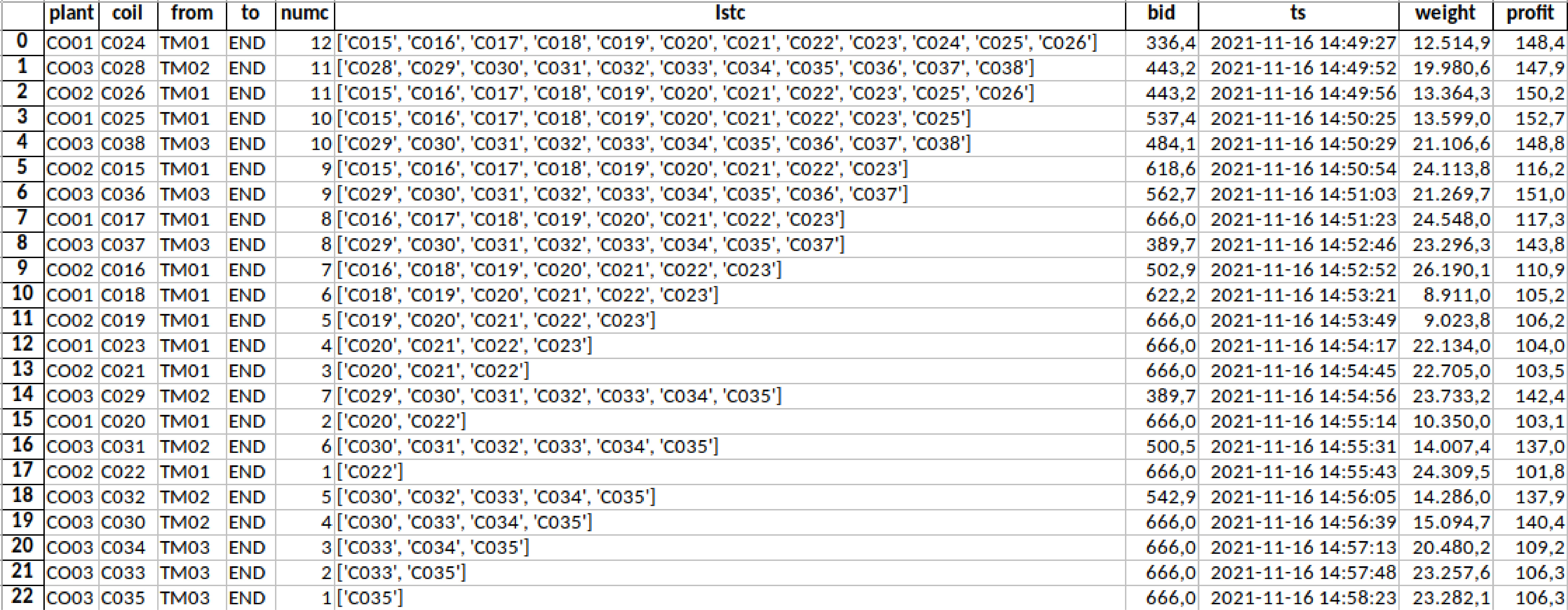
The structure of the job (orders) based outcome from the mid-term scheduling approach obtained for Coating plants are presented in Table 12. Each order is composed from 3 coils in this particular situation, where sequence accounts for the available time where the coils become ready for process at coating plants.
Figure 12.
Temporal scheduling for three coating plants where CO03 has its own list of demanding coils but CO01 and CO02 share demanding coils.
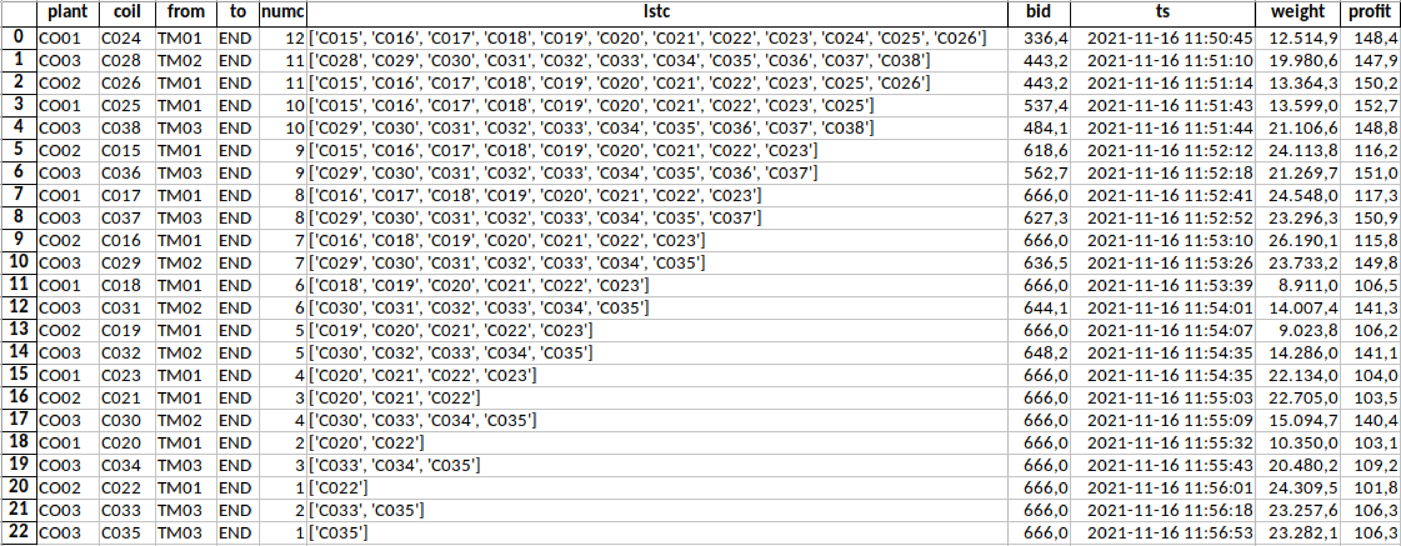
Figure 13.
Same situation than in Fig. 12 but where CO03 suffers a disruption for a period of time and later it becomes active again.
Because of the availability of coils through time, scheduling at local plants does not need to consider the whole set of coils because several of them will only be available at the plant later in time, which in practical terms means that a limited number of coils will be active per plant to participate in auctions (those effectively released from previous plants). Just in case, to avoid overloads because of the number of processes the MAS was designed to support different network attached computers running the agents. The negotiation platform is the single point where all the messages are exchanged. To make things easy, Log and Browser Agents have been placed at this node, where all the logging records are stored.
Regarding different experiments when number of coils waiting for a plant were between 5 and 30, the auction process allocates six auctions per minute and plant, with no dramatic degradation in response because of the major delays happen for message waiting (now set by 15 seconds granting any coil to decide if bidding or not). In addition, nothing is required if suddenly one coating plant becomes not available, provided that the mask of the targeted operation for coils enables several plants.
Another significant aspect is dealing with unex-pected plant unavailability periods. To simulate those different experiments have been conducted, first by enabling different plants to process coils according to their technical specifications, where the sequence of operations is indicated through regular expressions, allowing coils to hear auctions from different plants and enabling to continue processing when one plant has an issue. Therefore, in Fig. 12 the regular scheduling process is presented where plants CO01 and CO02 are targeted for order 326596–330151 and plant CO03 has its own orders. It can be seen how the scheduling time including bidding, counterbidding and resolution is faster for CO03 because coils do not need to wait different options looking to its higher benefit, which is the effect we can observe for CO01 and CO02. Indeed, regarding the profit in all the cases it grows from an initial level as coils losing competitions strength their options to win and such phenomenon is getting smaller through time. Figure 13 presents the case when a plant (CO03) went down during the scheduling (position 8), and it recovers later (position 14) without any additional human intervention. In this particular case, as far as the pending coils for CO03 have no options to apply to any other plants they must wait that plant to be recovered since the treatment is only carried out by that plant.
The MAS can be used not just for scheduling in the way it was introduced here, taking advance of the micro scheduling opportunities to consider extended factor criteria (when coils can get access to an energy forecast model from each plant, they can consider it in their auction), but also the MAS can be used for production control in such dynamic contexts.
6.Discussion and conclusions
The advantages of the hybrid method being proposed in this paper can be appreciated not only from a direct comparison to single algorithm-based techniques, no matter whether they are deterministic, stochastic or evolutionary based. The main advantage derives from the fact that none of the traditional approaches can provide efficient answers to the global capacity issues (stock limitation of WIP) in the long-term planning and at the same time provide flexible and efficient relocation of items when unexpected breakdowns happen, which are the most frequent events for the targeted industries (see Fig. 3).
Just to illustrate the direct impact, let us focus on the unexpected breakdowns, as the most frequent event on the collected sample for different industries. Therefore, just thinking in a synthetic scenario with different production plants processing different coils belonging to orders with different due dates, when the scheduling is carried out by the current tools and algorithms this means that coils to be processed in the plant having the incident become blocked until a new production plan is produced, which lasts between 0.5 and 1 hour. Then the new plan is launched, the breakdown becomes solved and another plan needs to be created. During the considered time slot of 1 to 2 hours production continued but potentially not in an optimal way, as no guidelines were available, which can drive the factory to violate due dates for specific orders or at least increase the risks of such an event. As far as those events happen many times per week, creation of new plans is a frequent activity impacting around 55 h/week. This high-capacity issue is further enhanced by the fact that the experts have different areas of expertise and means that the quality of the planning is linked to the individual skills of the experts. Since the new plans have to be created as quickly as possible, the focus is on plant utilization only. With the help of the proposed hybrid approach, situations that have arisen due to unforeseen events and require re-planning can be handled promptly by the short-term MAS, which will consider available coils to be processed in available plants, without significant waiting time. With reference to the example mentioned, employee capacities of approx. 55 h/week can thus be minimized and released, which leads to a gain in efficiency in the workflow-organizational processes as well as in the planning results by the optimization of the available plants and coils.
Based on the previous discussion, in the present work, a hybrid approach which combines three different strategies is proposed to deal with the production scheduling problem of an industrial CR use case for improving the flexibility of production scheduling. Each method has its own specific strengths and limitations: the CFM approach shows the lowest modelling precision referring to the planning granularity and cannot handle individual coils and/or orders, but is robust and fast in providing results with the highest forecasting ability (e.g. 1 month). The MOMILP is very useful and reliable in situations where the normal production flow is not affected by disturbances. It allows maximizing the capacity utilization providing nearly optimal solutions of the scheduling problem. Nevertheless, it faces difficulties in handling dynamic situations, and problem complexity and size may affect its solution time. Finally, the auction-based MAS approach enables short term local optimal decision-making process granting consideration for detailed production rules as per resource. It shows its flexibility in dynamic contexts, but it can provide suboptimal decisions from the global perspective. It requires close connection to the production resources, to be aware of unavailability of resources as well as process end-ups for coils.
Experimental results show that a proper combination of the methods allows merging the benefits of the single approaches while overcoming their drawbacks. The CFM provides a robust production planning for 1 month by managing the storages capacity and planned downtimes. The results of the CFM are then used to feed the MOMILP approach in order to satisfy daily production targets. The combination of MOMILP and auction-based MAS approaches provides both a proper and feasible resources scheduling for the upcoming 24 h and a reactive scheduling capable to adapt its behaviour in dynamic scenarios. Therefore, the flexibility of the production scheduling can be improved.
On the other hand, the maintainability of the final solution needs to be carefully considered for the industrial deployment.
There are several industrial sectors which can benefit from the adoption of the proposed method. More precisely, every real flexible/hybrid flow shop production, such as the metallurgical, chemical, glass, paper and food industries, which are characterized by the presence of different parallel machines in some or all stages, and by a partly continuous production cycle, i.e. the production runs 24 hours 7 days a week. Real flexible flow shop productions are dynamic and subject to a wide range of uncertainties ranging from machine breakdowns to rush orders. In order to handle such a complex dynamic environment, it is crucial to take advantage of several approaches with different scopes and granularities to deal with a wide range of uncertainties.
Future work will be focused on development and testing of the hybrid approach in different contexts, combining the results of all the methods, as well as on addressing practical aspects related to practical usability of the system in a physical industrial scenario. Future work also considers extending the auction criteria to include quality, energy demand as well as environmental aspects, as well as to consider different policies in all the time levels, to gain knowledge about the impact in terms of transparency and governance.
Acknowledgments
The research described in the present paper has been developed within the project entitled “Refinement of production scheduling through dynamic product routing, considering real-time plant monitoring and optimal reaction strategies (DynReAct)” (G.A. No 847203), which was funded by Research Fund for Coal and Steel (RFCS) of the European Union (EU). The sole responsibility of the issues treated in the present paper lies with the authors; the Commission is not responsible for any use that may be made of the information contained therein. The authors wish to acknowledge with thanks the EU for the opportunity granted that has made possible the development of the present work. The authors also wish to thank all partners of the project for their support and the fruitful discussion that led to successful completion of the present work.
Authors’ contributions
The role played by each author is synthesized according to CRediT (Contributor Roles Taxonomy) taxonomy.
Vincenzo Iannino: Conceptualization, Methodology, Software, Validation, Formal Analysis, Investigation, Data Curation, Writing – Original Draft Preparation, Writing – Review & Editing, Visualization.
Valentina Colla: Conceptualization, Methodology, Resources, Supervision, Funding Acquisition, Writing – Original Draft Preparation, Writing – Review & Editing.
Alessandro Maddaloni: Conceptualization, Methodology, Software, Formal Analysis, Investigation, Writing – Original Draft Preparation, Writing – Review & Editing.
Jens Brandenburger: Conceptualization, Methodology, Supervision, Project Administration, Funding Acquisition, Writing – Review & Editing.
Ahmad Rajabi: Conceptualization, Methodology.
Andreas Wolff: Conceptualization, Methodology, Software, Validation, Writing – Original Draft Preparation, Writing – Review & Editing.
Joaquin Ordieres: Conceptualization, Methodology, Software, Validation, Writing – Original Draft Preparation, Writing – Review & Editing.
Miguel Gutierrez: Conceptualization, Methodology, Validation, Formal Analysis, Writing – Review & Editing.
Erwin Sirovnik: Conceptualization, Writing – Original Draft Preparation, Writing – Review & Editing, Methodology, Project Administration, Funding Acquisition, Resources.
Dirk Mueller: Conceptualization, Supervision, Data Curation.
Christoph Schirm: Conceptualization, Data Curation, Formal Analysis.
References
[1] | Branca TA, Fornai B, Colla V, Murri MM, Streppa E, Schröder AJ. The challenge of digitalization in the steel sector. Metals (Basel). (2020) ; 10: (2): 1-23. |
[2] | Gajdzik B, Wolniak R. Transitioning of Steel Producers to the Steelworks 40 – Literature Review with Case Studies. Energies (2021) ; Vol 14, Page 4109. |
[3] | Colla V, Pietrosanti C, Malfa E, Peters K. Environment 4.0: How digitalization and machine learning can improve the environmental footprint of the steel production processes. Mater Tech. (2020) ; 108: (5-6): 1-11. |
[4] | Garey MR, Johnson DS. Computers and Intractability: A Guide to the Theory of NP-Completeness (Series of Books in the Mathematical Sciences). Comput Intractability. (1979) . |
[5] | Chiodini V. Configurable On-Line Scheduling. Integr Comput Aided Eng. (1996) Jan 1; 3: (4): 225-43. |
[6] | Harjunkoski I, Grossmann IE. A decomposition approach for the scheduling of a steel plant production. Comput Chem Eng. (2001) ; 25: (11-12): 1647-60. |
[7] | Karim A, Adeli H. CONSCOM: An OO Construction Scheduling and Change Management System. J Constr Eng Manag. (1999) ; 125: (5): 368-76. |
[8] | Senouci AB, Adeli H. Resource Scheduling Using Neural Dynamics Model of Adeli and Park. J Constr Eng Manag. (2001) ; 127: (1): 28-34. |
[9] | Lopez L, Carter MW, Gendreau M. The hot strip mill production scheduling problem: A tabu search approach. Eur J Oper Res. (1998) ; 106: (2-3): 317-35. |
[10] | Zhao J, Liu QL, Wang W. Models and algorithms of production scheduling in tandem cold rolling. Zidonghua Xuebao/Acta Autom Sin. (2008) ; 34: (5): 565-73. |
[11] | Valls Verdejo V, Alarcó MAP, Sorlí MPL. Scheduling in a continuous galvanizing line. Comput Oper Res. (2009) ; 36: (1): 280-96. |
[12] | Tang L, Zhang X, Guo Q. Two hybrid metaheuristic algorithms for hot rolling scheduling. ISIJ Int. (2009) ; 49: (4): 529-38. |
[13] | Rodrigues D, Papa JP, Adeli H. Meta-heuristic multi- and many-objective optimization techniques for solution of machine learning problems. Expert Syst. (2017) ; 34: (6). |
[14] | Gutierrez Soto M, Adeli H. Many-objective control optimization of high-rise building structures using replicator dynamics and neural dynamics model. Struct Multidiscip Optim. (2017) ; 56: (6): 1521-37. |
[15] | Ouelhadj D, Petrovic S. A survey of dynamic scheduling in manufacturing systems. J Sched. (2009) ; 12: : 417-31. |
[16] | Chaari T, Chaabane S, Aissani N, Trentesaux D. Scheduling under uncertainty: Survey and research directions. In: 2014 International Conference on Advanced Logistics and Transport, ICALT 2014. IEEE; (2014) . pp. 229-34. |
[17] | Iglesias-Escudero M, Villanueva-Balsera J, Ortega-Fernandez F, Rodriguez-Montequín V. Planning and scheduling with uncertainty in the steel sector: A review. Appl Sci. (2019) ; 9: (13): 1-15. |
[18] | Cowling PI, Ouelhadj D, Petrovic S. Dynamic scheduling of steel casting and milling using multi-agents. Prod Plan Control. (2004) ; 15: (2): 178-88. |
[19] | Ouelhadj D, Petrovic S, Cowling PI, Meisels A. Inter-agent cooperation and communication for agent-based robust dynamic scheduling in steel production. Adv Eng Informatics. (2004) ; 18: (3): 161-72. |
[20] | Gutierrez Soto M. and Adeli H. Multi-agent replicator controller for sustainable vibration control of smart structures. J Vibroengineering. (2017) ; 19: (6): 4300-4322. |
[21] | Ju Y, Tian X, Wei G. Fault tolerant consensus control of multi-agent systems under dynamic event-triggered mechanisms. ISA Trans. (2022) Jan 10. |
[22] | Iannino V, Mocci C, Colla V. A Brokering-Based Interaction Protocol for Dynamic Resource Allocation in Steel Production Processes. In: Rocha Á, Adeli H, Dzemyda G, Moreira F, Ramalho Correia A., editors. Trends and Applications in Information Systems and Technologies. Springer, Cham; (2021) . pp. 119-29. |
[23] | Guo Q, Tang L. Modelling and discrete differential evolution algorithm for order rescheduling problem in steel industry. Comput Ind Eng. (2019) ; 130: : 586-96. |
[24] | Tang L, Wang X. A predictive reactive scheduling method for color-coating production in steel industry. Int J Adv Manuf Technol. (2008) ; 35: : 633-45. |
[25] | Wang L, Zhao J, Wang W, Cong L. Dynamic scheduling with production process reconfiguration for cold rolling line. IFAC Proc Vol. (2011) ; 44: (1): 12114-9. |
[26] | Hou DL, Li TK. Analysis of random disturbances on shop floor in modern steel production dynamic environment. Procedia Eng. (2012) ; 29: : 663-7. |
[27] | Abdulmohsen AM, Omran WA. Active/reactive power management in islanded microgrids via multi-agent systems. Int J Electr Power Energy Syst. (2022) ; 135: (107551): 1-10. |
[28] | Hong Y, Wang X. Robust operation optimization in cold rolling production process. In: 26th Chinese Control and Decision Conference, CCDC 2014. Changsha, China: IEEE; (2014) . pp. 1365-70. |
[29] | Álvarez-Gil N, Álvarez García S, Rosillo R, de la Fuente D. Sequencing jobs with asymmetric costs and transition constraints in a finishing line: A real case study. Comput Ind Eng. (2022) Mar 1; 165: : 107908. |
[30] | Nastasi G, Colla V, Del Seppia M. A multi-objective coil route planning system for the steelmaking industry based on evolutionary algorithms. Int J Simul Syst Sci Technol. (2015) ; 16: (1): 6.1-6.8. |
[31] | Mori J, Mahalec V. Planning and scheduling of steel plates production. Part I: Estimation of production times via hybrid Bayesian networks for large domain of discrete variables. Comput Chem Eng. (2015) ; 79: : 113-34. |
[32] | thyssenkrupp R. Wege der Produktion. Brochure. (2015) . https//www.thyssenkrupp-steel.com/media/content_1/publikationen/packaging_steel_1/wege_der_produktion_process_routes_thyssenkrupp_packaging_steel.pdf. |
[33] | Pinedo ML. Scheduling: Theory, algorithms, and systems. Scheduling: Theory, Algorithms, and Systems. (2008) . |
[34] | Rokni S, Fayek AR. A multi-criteria optimization framework for industrial shop scheduling using fuzzy set theory. Integr Comput Aided Eng. (2010) Jan 1; 17: (3): 175-96. |
[35] | Kiran DR. Production planning and control: A comprehensive approach. Production Planning and Control: A Comprehensive Approach. (2019) . |
[36] | Schönsleben P. Integrales Logistikmanagement: Operations und Supply Chain Management in umfassenden Wertschöpfungsnetzwerken. Integrales Logistikmanagement. Springer Vieweg; (2020) . |
[37] | Meudt T, Wonnemann A, Metternich J. Produktionsplanung und-steuerung (PPS) – ein Überblick der Literatur der unterschiedlichen Einteilung von PPS-Konzepten. Darmstadt; (2017) . https//tuprints.ulb.tu-darmstadt.de/6654/. |
[38] | Suri R, Fu BR. On using continuous flow lines to model discrete production lines. Discret Event Dyn Syst Theory Appl. (1994) . |
[39] | Sun L, Qu D, Liu G. A mixed integer programming model for gas distribution problem with complex gas applied characteristics. J Comput Methods Sci Eng. (2016) Jan 1; 16: (4): 865-75. |
[40] | Maddaloni A, Colla V, Nastasi G, Del Seppia M, Iannino V. A Bin Packing Algorithm for Steel Production. In: Proceedings – UKSim-AMSS 2016: 10th European Modelling Symposium on Computer Modelling and Simulation. Pisa: IEEE; (2017) . pp. 19-24. |
[41] | Maddaloni A, Porzio GF, Nastasi G, Colla V, Branca TA. Multi-objective optimization applied to retrofit analysis: A case study for the iron and steel industry. Appl Therm Eng. (2015) Dec 5; 91: : 638-46. |
[42] | Matino I, Colla V, Branca TA, Romaniello L. Optimization of By-Products Reuse in the Steel Industry: Valorization of Secondary Resources with a Particular Attention on Their Pelletization. Waste Biomass Valorization. (2017) ; 8: (8): 2569-81. |
[43] | Heydarabadi H, Doniavi A, Babazadeh R, Azar HS. Optimal production-distribution planning in electromotor manufacturing industries: A case study. Int J Adv Oper Manag. (2020) ; 12: (1): 1-27. |
[44] | Özgüven C, Özbakir L, Yavuz Y. Mathematical models for job-shop scheduling problems with routing and process plan flexibility. Appl Math Model. (2010) Jun 1; 34: (6): 1539-48. |
[45] | Hwang C-L, Yoon K. Multiple Attribute Decision Making Methods and Applications A State-of-the-Art Survey. 1st ed. Lecture Notes in Economics and Mathematical Systems. Springer-Verlag Berlin Heidelberg; (1981) . |
[46] | Hadera H, Harjunkoski I, Sand G, Grossmann IE, Engell S. Optimization of steel production scheduling with complex time-sensitive electricity cost. Comput Chem Eng. (2015) ; 76: : 117-36. |


