Data Augmentation for Classification of Multi-Domain Tension Signals

Žvirblis, Tadas; Pikšrys, Armantas; Bzinkowski, Damian; Rucki, Mirosław; Kilikevičius, Artūras; Kurasova, Olga

doi:10.15388/24-INFOR578

Data Augmentation for Classification of Multi-Domain Tension Signals

Article type: Research Article

Authors: Žvirblis, Tadas^{1; ∗} | Pikšrys, Armantas² | Bzinkowski, Damian³ | Rucki, Mirosław³ | Kilikevičius, Artūras⁴ | Kurasova, Olga¹

Affiliations: [1] Institute of Data Science and Digital Technologies, Vilnius University, Lithuania | [2] Institute of Computer Science, Vilnius University, Lithuania | [3] Faculty of Mechanical Engineering, Kazimierz Pułaski University of Technology and Humanities in Radom, Poland | [4] Institute of Mechanical Science, Vilnius Gediminas Technical University, Lithuania

Correspondence: [∗] Corresponding author.

Keywords: fully convolutional network, convolutional neural network, long short-term memory model, residual networks, inception networks, data augmentation, sliding window, magnitude warping, variational autoencoder, conveyor belt tension signals

DOI: 10.15388/24-INFOR578

Journal: Informatica, vol. 35, no. 4, pp. 883-908, 2024

Received August 2024

Accepted November 2024

Published: 2024

Get PDF

Abstract

There are different deep neural network (DNN) architectures and methods for performing augmentation on time series data, but not all the methods can be adapted for specific datasets. This article explores the development of deep learning models for time series, applies data augmentation methods to conveyor belt (CB) tension signal data and investigates the influence of these methods on the accuracy of CB state classification. CB systems are one of the essential elements of production processes, enabling smooth transportation of various industrial items, therefore its analysis is highly important. For the purpose of this work, multi-domain tension data signals from five different CB load weight conditions (0.5 kg, 1 kg, 2 kg, 3 kg, 5 kg) and one damaged belt condition were collected and analysed. Four DNN models based on fully convolutional network (FCN), convolutional neural network combined with long short-term memory (CNN-LSTM) model, residual network (ResNet), and InceptionTime architectures were developed and applied to classification of CB states. Different time series augmentations, such as random Laplace noise, drifted Gaussian noise, uniform noise, and magnitude warping, were applied to collected data during the study. Furthermore, new CB tension signals were generated using a TimeVAE model. The study has shown that DNN models based on FCN, ResNet, and InceptionTime architectures are able to classify CB states accurately. The research has also shown that various data augmentation methods can improve the accuracy of the above-mentioned models, for example, the combined addition of random Laplace and drifted Gaussian noise improved FCN model’s baseline (without augmentation) classification accuracy with 2.0 s-length signals by 4.5% to 92.6% ± 1.54%. FCN model demonstrated the best accuracy and classification performance despite its lowest amount of trainable parameters, thus demonstrating the importance of selecting and optimizing the right architecture when developing models for specific tasks.

1Introduction

With the rapid development of deep learning (DL), the issue of insufficient datasets has become increasingly prominent. The performance of deep neural networks (DNN) is particularly dependent on the quantity, quality, and variety of training data (Sarker, 2021). This problem is particularly evident in mechanical engineering, where machine learning (ML) is widely used. In experimental scenarios, obtaining sufficient data to train robust models can be difficult and expensive. The reliance on large datasets for training DL models highlights the need for obtaining sufficient data while lowering data collection costs.

Our research paper focuses on applying DL models to the classification of conveyor belt (CB) states (damaged CB and loaded with 0.5 kg, 1 kg, 2 kg, 3 kg, or 5 kg), specifically using belt tension time series signals. DL methods for the classification of CB states using images have been widely researched already, but the methods for classifying CB tension signals remain limited. Previous studies have demonstrated the potential of DL models like LSTM for this purpose (Žvirblis et al., 2022).

In the industrial sector, CB systems is one of the essential elements of production processes, enabling smooth transportation of various items. Depending on specific industrial application, CB systems must meet certain criteria and requirements, such as sterility in the food industry (Klištincová et al., 2024) or high wear resistance and durability (Bortnowski et al., 2022b). The reliability and efficiency of these conveyors are important to optimize work processes and avoid unplanned stops. An integral aspect of the maintenance of conveyor systems is monitoring their operational status to ensure correct functioning of the system and timely detection of potential faults (Dąbek et al., 2023). Traditional CB monitoring methods, such as manual, spectral, or radiographic damage detection (Li et al., 2011), are usually too expensive or require a lot of manual labour and are prone to human error.

Monitoring the status of CB systems is a critical aspect of their operational efficiency and safety. In the past, classification tasks in this area were performed using conventional ML algorithms and shallow models such as logistic regression and decision trees (Andrejiova et al., 2021). Over the last decade, DL methods have been applied increasingly widely because of their higher accuracy and efficiency. Santos et al. (2020) introduced binary classification models which used CB images. Classification was performed using deep convolutional neural networks (CNN) such as the visual geometry group (VGG) network, residual network (ResNet), and densely connected convolutional network (DenseNet). The highest average classification accuracy (89.8%) for particular data was achieved using DenseNet model. Zhang et al. (2021) performed a detailed analysis of ML algorithms and a comparison of DL models such as region-based CNN (R-CNN), single-shot detector (SSD), receptive field block net (RFBNet), Yolov3, and Yolov4 for the classification of CB damage images. Improved by the latter authors, Yolov3 architecture achieved an average classification accuracy of 97.3% for four damage classes.

Recent research has further revealed the application potential of DNNs in CB monitoring systems. Wang et al. (2023) presented a computer vision model capable of identifying CB defects with 94% accuracy, but this model was very sensitive to environmental effects and image quality. In another study, Bortnowski et al. (2022a) presented a long short-term memory (LSTM) autoencoder for automatization of damage detection by using recorded CB vibration signals. However, this model was not adapted to detect different types of CB damage. In addition, the vibration signals used in the study may be volatile due to various factors, such as load conditions or conveyor operating speed, which may affect the accuracy of the monitoring system.

CB tension signal data was applied to train various ML and DL models by Žvirblis et al. (2022) to determine the minimum signal length while maintaining high classification accuracy. However, in the study, DL models were only applied to classify two CB states (loaded with a 2 kg weight and unloaded). The authors did not include the detection of CB damage. Also, in the study, the initial dataset of CB tension signals was insufficient to train the models, so the authors performed two data augmentations methods like addition of random Laplace noise and drifted Gaussian noise. However, the main aim of the above-mentioned study was to develop high-accuracy classification models.

Achieving high classification accuracy with certain DL models requires collecting a sufficiently large and diverse dataset. Collecting large amounts of CB tension time series data can be difficult and expensive, therefore data augmentation methods can be used to increase the amount and variety of data. Data augmentation involves the creation of new data that is modified or synthesized from the original dataset. This enables the model to better generalize data and recognize features in unseen data. Data augmentation techniques are widely studied in computer vision and natural language processing, but their application to time series data is still being developed.

For time series data, traditional image augmentation methods such as scaling, rotating, or cropping often are not suitable due to the time dependence of time series data. Improper time series augmentations can negatively affect the accuracy and robustness of the model in real-world scenarios. In research works, some of the most effective time series data augmentation methods were the application of a sliding window, the addition of noise, and the synthesis of data using variational autoencoders (VAE) (Kingma and Welling, 2019) or generative adversarial networks (GAN) (Goodfellow et al., 2014).

Data augmentation methods in DL are used to find effective strategies for improvement of the accuracy and robustness of models while having limited or unbalanced datasets. Recently, some scientific works related to data augmentation were published (Chlap et al., 2021; Wang et al., 2017a). However, most of these works provided applications for the areas related to image augmentation in computer vision models.

Further below, this work reviews various time series data augmentation methods that could augment the time series dataset and potentially improve the classification accuracy and robustness of DL models.

Raw time series data usually forms one long time series. The sliding window method can be used to generate more data for training. This augmentation method was used by Žvirblis et al. (2022) in a study where the initial CB tension signal data was divided into two stages. In the first stage, a sliding window method was used to divide the original signal into smaller signals and thereby expand the dataset. One of the disadvantages of a sliding window method is that dividing the original signal into smaller signals can cut off important features of time series data. Because of this, a DL model may not learn properly to classify small-window-size time series data.

Additional noise in the data simulates real data, as real equipment such as signal sensors can introduce noise into the observations. Therefore, adding noise makes DL models more robust to small variations in the data. Laplace, drifted Gaussian, and uniform noise are commonly used for augmentation of time series data (Um et al., 2017; Iwana and Uchida, 2021; Žvirblis et al., 2022). However, adding too much noise to the original dataset can hinder the DL model’s ability to extract features from the signal. For this reason, it is important to study the influence of different amounts of noise on the model’s classification accuracy.

In augmentation of time series data, scaling means changing the amplitude or size of the original time series. Scaling augmentation methods for time series include magnitude warping, time warping, window warping, and frequency warping (Iwana and Uchida, 2021; Um et al., 2017). However, these augmentations can over-distort important features of time series data, so it is important to choose the methods appropriate for a specific dataset.

VAEs can be used for augmentation of time series data as well (Kingma and Welling, 2019; Goubeaud et al., 2021). Desai et al. (2021) presented the architecture of time series data variational autoencoder (TimeVAE), which was compared with other time series synthesis models such as TimeGAN (Yoon et al., 2019). On the average, the presented TimeVAE architecture showed higher accuracy of time series data synthesis than other models, especially with small data sets.

GANs is another widely researched framework for data augmentation and data synthesis, including time series data (Goodfellow et al., 2014). The architecture of GANs learns the distribution of data by extracting key features of the data. A trained generator of this architecture can then synthesize completely new data.

Currently, there are many different uses of GAN architectures for time series data (Huang et al., 2023; Iglesias et al., 2023). TimeGAN, one of the most widely used GAN architectures for time series, adds two new embedder and recovery networks to the conventional generator and discriminator architecture (Yoon et al., 2019). These new embedding and retrieval networks form an autoencoder in TimeGAN architecture that aims to learn the time dependence and key features of the data. In TimeGAN architecture, the autoencoder uses a recovery loss function, which aims to ensure that the network can accurately recover the original time series data from the latent space.

Conditional GANs contribute to traditional architectures by incorporating conditional information into the training process. This allows the network to be trained to generate more accurate data based on specific inputs, such as classes of data. The conditional GAN time series architecture (TSGAN) has achieved higher accuracy in synthesizing time series data for classification tasks than other GAN architectures (Smith and Smith, 2020). TSGAN architecture was tested on 70 datasets and compared with Wasserstein Generative Adversarial Network (WGAN) architecture (Gregor Hartmann et al., 2018). The accuracy of the data synthesized by TSGAN architecture was higher than that of WGAN architecture by about 11% on the average.

There are different DNN architectures and methods for performing augmentations on time series data, but not all the methods can be adapted for specific datasets. This work aims to develop DL models for time series, apply data augmentation methods to CB tension signal data and investigate the influence of these methods on the accuracy of CB state classification.

The rest of the paper is organized as follows. Materials and methods are described in Section 2. The main study results are provided in Section 3. Conclusions close the paper in Section 4.

2Materials and Methods

The aim of the study on the classification of load and defect states of a CB is to not only compare the classification accuracy of different DNN models but also to compare how the accuracy of the models is affected by different data augmentation methods. This chapter examines selected time series data augmentation methods that will be applied to CB tension signals as well as selected DL models, accuracy metrics, and data acquisition.

2.1Experimental Design and Data Collection

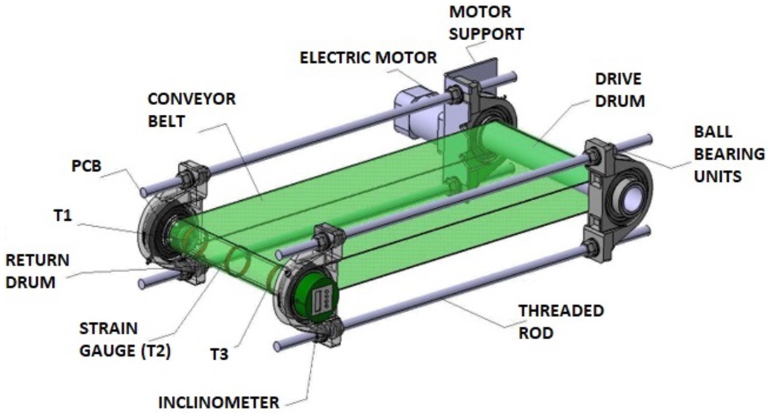
The test stand, on which the measurements were carried out, was a CB model, shown in Fig. 1. Its supporting structure consists of four self-aligning ball bearing units and two drums are embedded in the inner raceways: drive and return, on which strain gauges T1, T2, and T3 are located. The housings were connected by threaded rods and bolted with nuts, and sets of lenticular washers were used between the surfaces of the bearing housings on both sides to compensate for curvature.

Fig. 1

CB model.

The system uses strain gauges, in which the resistance RT depends directly on the resultant belt force Fn. During the dynamic testing of the CB (Fig. 2), the speed of the drive drum is set at v and the recorded waveforms of the signals from the strain gauges depend on the pre-tension of the belt, longitudinal damage UW, transverse damage UP, and the load m. The strain gauge sensors have nonlinear characteristics, and there is a nonlinear dependence of the readings depending on where the belt is pressed on the belt strain gauge which girds the shaft. The analog-to-digital converter (ADC) electronic circuit receives the analog data and converts it to digital, and then sends it via Bluetooth transmission to a computer. At the stage of converting analog values to digital, the signal is discretized and its values are measured at a frequency of 200 Hz. The signal, which goes to the computer in digital form, is represented in analog-to-digital units (ADUs) and the acquired values are subject to rounding and linearization.

Fig. 2

CB condition monitoring system.

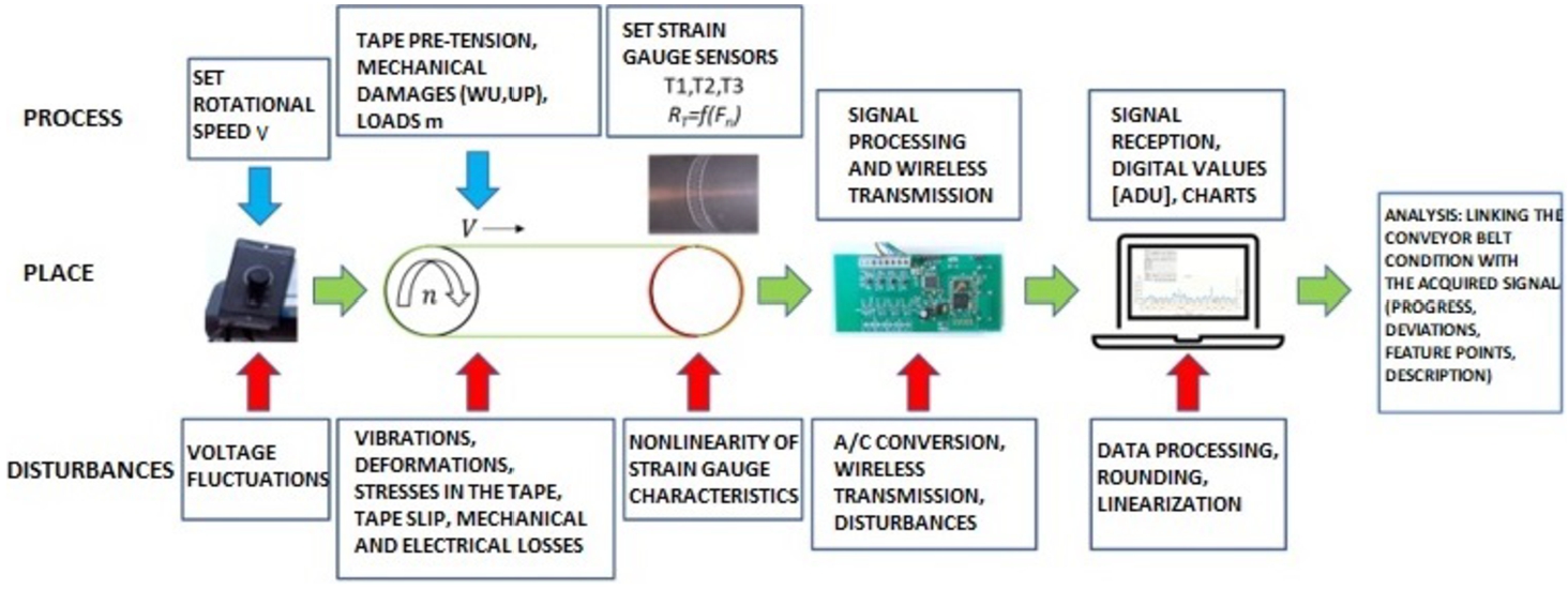
Fig. 3

CB damage diagram. Here UW I is a longitudinal cut of 50 mm, UW II is a longitudinal cut of 70 mm, UW III is a longitudinal cut of 45 mm with a depth of 1 mm, UW IV is a longitudinal cut of 50 mm with a depth of 1.5 mm and UP I is a cross cut of 10 mm.

The main purpose of data collection was to observe and analyse the influence of various belt loads and defects on CB tension signals. The observations were collected by using three strain gauge sensors, which were placed in parallel at different sections of the CB (top, middle, and bottom) to fully record the strain signal of the CB. For this reason, further data collection, analysis, and model building were done on multi-domain data input structure. Observations were carried out in two stages. In the first stage, observations were made by using the conveyor loaded with one of five different weights: 0.5 kg, 1 kg, 2 kg, 3 kg, or 5 kg. Each weight category was designed to simulate different loading conditions on the CB. In the second stage, CB was intentionally damaged in certain places to simulate defects in real conditions as shown in Fig. 3. During the second stage of observations, CB tension signals were recorded as in the case of belt damage without any weight load.

Fig. 4

Sensor signal values in different conditions of the conveyor belt: a) first lower sensor; b) second middle sensor; c) third upper sensor.

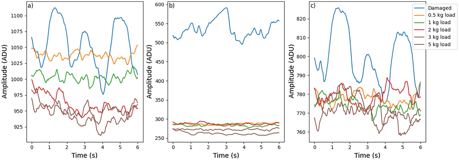
Fig. 5

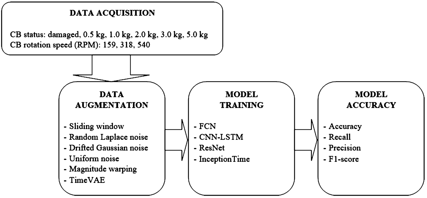
The scheme of experiment.

To simulate different rotational speeds of the CB, three different revolutions per minute (RPM) speeds were chosen: 159, 318, and 540. The CB speed of 159 RPM corresponded to a linear speed of 0.5 m/s, 318 RPM corresponded to 1 m/s, and 540 RPM corresponded to 1.7 m/s. Each observation was performed 9 times (3 times for each RPM). All the observations lasted about 8 seconds each on the average.

To gain more insight into the collected data, the amplitude means of the tension signals under different weight loads and defect states were calculated and presented in Fig. 4. The damaged CB signal has the highest average amplitude of all the load conditions, therefore it is clearly identifiable. Higher amplitude can be explained by the presence of defects and irregularities on the surface of the CB, which cause larger fluctuations in the tension signals. It can also be observed that the average tension amplitude of the maximum weight load of 5 kg was the lowest while that of 0.5 kg was the highest as compared with other weight loads.

Augmentation of the collected data and other steps of the experiment are shown in Fig. 5.

2.2Data Augmentation Techniques

Testing a wide range of data augmentation techniques is crucial in DL because different augmentations can have varied and sometimes profound impacts on model performance, generalization, and robustness. Data augmentation helps to prevent overfitting by exposing the model to diverse data transformations, which simulates the variability it may encounter in real-world scenarios. Different data types or domains may benefit from specific augmentations. For instance, noise injections can be useful for vibration or sound data. Testing various augmentations helps identify those that address domain-specific challenges effectively, enhancing the model’s adaptability.

We applied a range of data augmentation techniques, both traditional and advanced. These included:

• Basic augmentations: sliding window.
• Advanced augmentations: random Laplace noise, drifted Gaussian noise, uniform noise, and magnitude warping.
• Generative augmentations: variational autoencoders.

A sliding window splits the data into more time series of smaller sizes. The sliding window formula used in this work is:

W[i]=[1+i,m+i],i=0,1,2,…,k−m,

where a time series of size k is split into multiple time series of length m. Here, W[i] represents the i-th window, starting with index 1+i and ending with index m+i.

To expand the dataset of CB signals and to standardize their length, signals of all original observations were divided into 0.5 s (200 points), 1.0 s (400 points), and 1.5 s (600 points) signals. The step of each signal’s sliding window was 100% of the window size itself. For example, a step of 0.5 s-length signal is 0.5 s (200 points). This was done to create enough of different signals for training the models and to avoid over-fitting the models.

Random Laplace noise is based on sampling random values from a Laplace distribution. This distribution is characterized by the Laplace probability density function:

f1(x)=12σe−|x−μ|σ,

where μ is the mean of the distribution, and σ is the scale parameter controlling the width of the distribution.

Drifted Gaussian noise adds a random value from a Gaussian (normal) distribution to each point in the signal. Gaussian distribution is characterized by Gaussian probability density function:

f2(x)=1σ2πe−12(x−μσ)2,

where μ is the mean of the distribution and σ is the standard deviation.

Uniform noise generates a value from a uniform distribution. The uniform distribution is characterized by the density function that represents the equal likelihood of any value within the specified interval [a;b]:

f(x)=1b−a,a⩽x⩽b,0,x<aorx>b.

where a and b are the lowest and highest value of x, respectively.

Magnitude warping for time series data involves the random scaling of certain segments of the data. To perform the deformations, nodes u=u1,u2,…,ui are generated randomly from a Gaussian distribution. The scaling is then defined by cubic spline interpolation of the nodes S(x) (Iglesias et al., 2023). The magnitude warping function is represented by the formula:

x0(α)={α1x1,…,αtxt,…,αTxT},

where α={α1,α2,…,αi}=S(x), S(x) is cubic spline interpolation of the knots.

TimeVAE architecture is one more of the methods for data augmentation of CB tension signals (Desai et al., 2021). TimeVAE architecture is trained using the evidence lower bound (ELBO) loss function:

Lθ,ϕ=−Eqϕ(z|x)[logpθ(x|z)]+DKL(qϕ(z|x)||pθ(z)),

where the first term −Eqϕ(z|x)[logpθ(x|z)] is the reconstruction loss, which measures how accurately the model reconstructs the input data. It includes the log-likelihood for the variable z drawn from the distribution qϕ(z|x), where qϕ(z|x) is the encoded latent space for the variable x. The second term DKL(qϕ(z|x)||pθ(z)) is the Kullback-Leibler deviation between qϕ(z|x) and pθ(z) distributions. This regularization term is meant to ensure that the learned latent space remains similar to the prior distribution. In TimeVAE architecture, the variable z is taken from a Gaussian distribution and passed to the decoder, thus making the VAE decoder generative.

The encoder passes the input through a one-dimensional convolutional layer with ReLU activation function. The input is flattened and then connected to the output from the encoder’s fully connected layer. The encoder output parameters are used for constructing Gaussian distribution from which the variable z is derived. This variable is then passed to the decoder, which consists of fully connected, convolution, and time-distributed concatenation layers. The output data from the decoder is the same shape as the input data.

2.3Deep Learning Models Architectures

Multiple DL models were tested in order to ensure the broad applicability of findings, including fully convolutional network (FCN), convolutional neural network combined with long short-term memory network (CNN-LSTM), residual network (ResNet), and inception network (InceptionTime). All the models were built to classify six CB states, which included five load conditions (0.5 kg, 1 kg, 2 kg, 3 kg, and 5 kg) and one damaged-belt condition.

All the models were built using the Python programming language with TensorFlow and Keras DL libraries. The Kaggle platform was used for executing the experiments, and the NVIDIA Tesla P100 graphics processor was used for model training. In addition, each model was trained using the cross-entropy loss function and the Adam optimizer with a training rate of η=0.001. The following subsections present detailed architecture and parameter configuration of each constructed model.

2.3.1FCN Model

FCN is an architecture based on deep CNNs that were originally developed for image segmentation (Long et al., 2015). In the case of time series, FCN architecture can be used for feature extraction. In the output layer, the classification can be performed using either the exponential normalization (softmax) or the sigmoid activation function (Wang et al., 2017b). The basic block of FCN architecture consists of a convolutional layer, followed by a batch normalization layer and a rectified linear unit (ReLU) activation layer. During the training, the batch normalization layer accelerates gradient convergence and improves the model’s robustness. Batch normalization is given by the following formula:

BN(x)=x−μσ2+ϵ×γ+β,

where x is the input, μ is the mini-batch mean, σ is the mini-batch standard deviation, ϵ is the numerical stability constant, γ is the learned scale parameter, and β is the learned shift parameter.

The mathematical expression of FCN architecture block is given in formulas (1), (2), and (3):

(1)

z=W∗x+b,

(2)

y=BN(z),

(3)

h=ReLU(y),

where ∗ denotes the convolution operation, x is the input data, W is the convolution layer kernel, b is the bias, BN denotes the batch normalization operation, and ReLU is rectified linear unit operation.

The final FCN is formed by concatenating three convolutional blocks. After applying these blocks, the extracted data features are passed to the global average pooling (GAP) layer, which is responsible for reducing the feature map size (Hsiao et al., 2019). GAP layer is superior to the traditional fully connected layer because it significantly reduces the number of weights and helps the model avoid over-training. The final layer consists of the softmax or sigmoid activation function.

The architecture of the built FCN model is shown in Fig. 6. The developed model is composed of three one-dimensional convolutional layers with the number of filters 64, 128, and 64, respectively. The filter size of each convolutional layer was 3×1. The selection of 64, 128, and 64 filters was made based on findings in previous studies that demonstrated good accuracy in time series classification tasks using similar FCN model (Wang et al., 2017b). The final layers consist of a GAP layer and a fully connected layer with a softmax activation function. The resulting FCN model was the smallest among all the models built in this study as it consisted of only 26437 trainable parameters.

Fig. 6

FCN model architecture.

2.3.2CNN-LSTM Model

The architecture and parameter configuration of the second hybrid CNN-LSTM model is shown in Fig. 7. The developed model is composed of four different one-dimensional convolutional blocks and two LSTM layers. The number of convolutional block filters in the model decreases from 512 to 8, respectively. Convolutional blocks use batch normalization, ReLU activation function, average pooling, and dropout layers. The number of convolutional filters was empirically tested with various configurations, and the chosen structure provided optimal classification accuracy. The convolutional blocks are followed by two LSTM layers, each composed of 16 cells. The final layer is fully connected and utilizes the softmax activation function. The trainable parameters of the created CNN-LSTM model ranged from 226.077 with 0.5 s-length signals to 245.533 with 2.0 s-length signals.

Fig. 7

CNN-LSTM model architecture.

2.3.3ResNet Model

The architecture and parameter configuration of ResNet model is shown in Fig. 8. The model consists of three residual blocks. In the first residual block, each of one-dimensional convolutions has 64 filters and in the second and third, 128. The selected filter sizes were based on previous studies that applied ResNet architecture for time series classification (Wang et al., 2017b). In the architecture diagram of the model, arrows with a plus sign represent skip connections. The last two layers of the model consist of a GAP layer and a fully connected layer with a softmax activation function. The developed ResNet model had the largest number of parameters among all the built models and consisted of 508.357 trainable parameters.

2.3.4InceptionTime Model

The architecture and parameter configuration of the InceptionTime model with six inception modules is shown in Fig. 9. Every third module is connected by ResNet skip connections. The final two layers of the model include a GAP layer and a fully connected layer with a softmax activation function. The InceptionTime model has a total of 427.685 trainable parameters.

Fig. 8

ResNet model architecture.

Fig. 9

Inception network InceptionTime model architecture.

2.4Classification Accuracy Metrics

Overall classification accuracy measures overall accuracy of the model. It is the ratio of correct guesses to all guesses. The overall accuracy in percent is represented by the formula:

Accuracy=TP+TNTP+FN+FP+TN·100%,

where TP represents true positives, TN represents true negatives, FP represents false positives, and FN represents false negative model results.

The accuracy of each experiment was measured more than once, so it is important to estimate the error in order to evaluate the data from these samples of different accuracy. By calculating the standard error (SE) of the mean, it is possible to assess the extent to which the sample is representative of the population and draw reasonable conclusions from it. SE was calculated by the formula:

SE=sn,

where s is the sample standard deviation and n is the sample size.

Classification accuracy alone can lead to misinterpretation of results when the dataset is unbalanced. For this reason, depending on the classification results of the classification model, recall and precision metrics of the model can also be calculated. These metrics are represented as percentages:

Recall=TPTP+FN·100%,Precision=TPTP+FP·100%,

where recall shows whether the model can predict all the instances of different classes and precision shows how often the positive predictions are correct.

In addition, F1-score, which is a weighted average of recall and precision, can be used to determine the classification accuracy in the case of unbalanced datasets. This metric is expressed as a percentage in the formula:

F1=2·Recall·PrecisionRecall+Precision·100%,

where Recall is the proportion of actual positives that were correctly identified and Precision is the proportion of predictions that were correct.

3Results and Discussion

In this section, a study on the accomplished classification of CB load and defect states is provided. First, DNN models were built. Various time series data augmentation methods were then applied to the dataset and comparisons of the original and augmented signals were made. Finally, a study of conveyor state classification was carried out by using the constructed DNN models and various data augmentation methods. The results of all the studied methods were compared and the conclusions were drawn. The DNN models, augmentation methods, and data used in the study are available in the GitHub repository.1 1

3.1Application of Data Augmentations

Data augmentation was performed on the CB tension signals before analysing the CB state classification accuracy. All the applied data augmentation methods are presented in this section.

Table 1

Sliding window signals.

Signal length (s)	Data points	Signal count
0.5	200	1.058
1.0	400	514
1.5	600	319
2.0	800	233

3.1.1Sliding Window

A sliding window was applied to the raw tension signals to generate datasets of four different lengths: 0.5 s (200 points), 1.0 s (400 points), 1.5 s (600 points), and 2.0 s (800 points). The step size of each sliding window was 100% of the signal’s length. The number of signals for each length is presented in Table 1. The shortest-signal (0.5 s) dataset was the biggest (1.058), while that of the longest signal (2.0 s) was the smallest (233). These signals of different lengths were used in further time series data augmentation and classification accuracy studies. Additionally, the signals were normalized before applying data augmentations.

Fig. 10

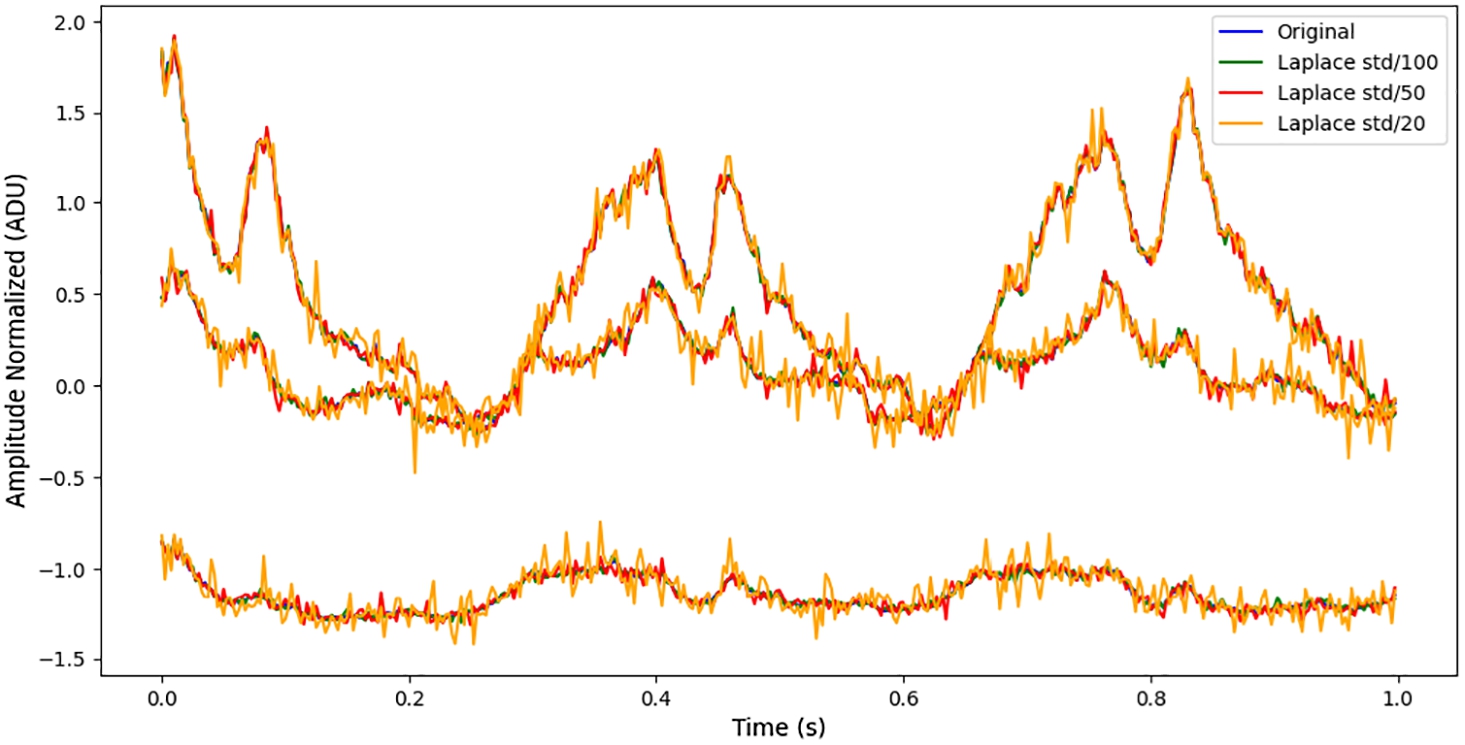
Comparison of different scale random Laplace noise with the original signal.

3.1.2Noise Addition

Various types of noise such as random Laplace, drifted Gaussian, or uniform noises were added to the processed tension signal data. The scale of the noise was determined by the standard deviation (std) of the original signal. The different scales of noise were generated by scaling the standard deviation of the original signal to fractions of its value: std/100, std/50, and std/20. This scaling adjusts the noise magnitude, with smaller proportions (e.g., std/100) representing lower noise levels and larger proportions (e.g., std/20) introducing higher noise, all in proportion to the original signal’s variability. Figure 10 presents a comparison between the original tension signal and the one augmented with random Laplace noise at different scales. As can be seen, the signal becomes progressively noisier as the noise scale increases from std/100 to std/20, demonstrating how higher magnitudes introduce more fluctuations while preserving the overall structure of the original signal.

Fig. 11

Comparison of random Laplace and drifted Gaussian noise combinations with the original signal.

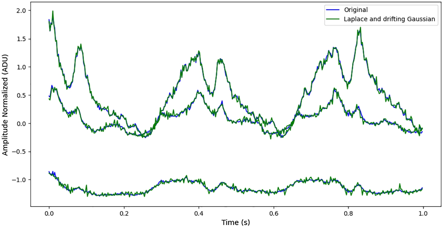
Noise addition data augmentations were performed by using various noise combinations. Random Laplace noise was combined with drifted Gaussian noise and uniform noise, each with a magnitude of std/100. Figure 11 compares the original signal with the combination of random Laplace and drifted Gaussian noise. The use of both Laplace and drifted Gaussian noise introduces a combination of sharp, sudden deviations (characteristic for Laplace noise) and smoother, gradual deviations (characteristic for Gaussian noise). The comparison shows that the augmented signal retains the major trends of the original signal, while the addition of noise results in slight amplitude variations.

3.1.3Magnitude Warping

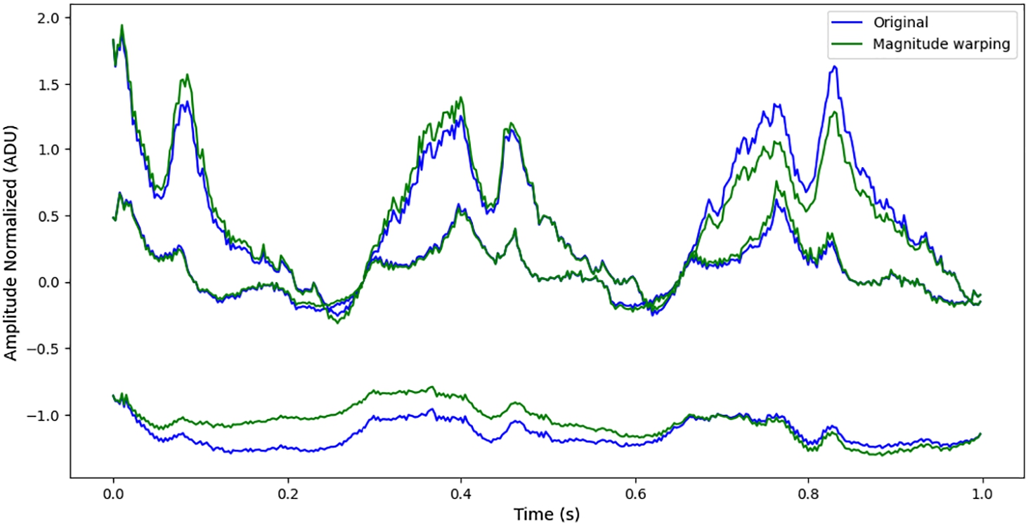
Magnitude warping was applied to the processed tension signals. Deformation parameter σ=0.2 and 4 nodes were used for the deformation function. The comparison of the original and deformed signal is shown in Fig. 12. The warped signal showed noticeable changes in amplitude as compared to the original signal. Despite these amplitude modifications, the main features and overall trends of the original signal remained intact, making this method suitable for creating variations of the original data without altering the core structure.

Fig. 12

Comparison of magnitude warping with the original signal.

3.1.4Variational Autoencoder Signal Generation

Fig. 13

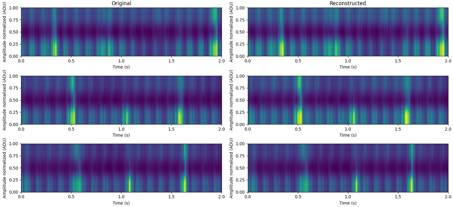
Comparison of original and reconstructed signals.

Processed tension signals were used to train TimeVAE model with three hidden layers containing 50, 100, and 200 neurons, respectively, and 20 neurons in the latent space. The selection of 50, 100, and 200 neurons for the hidden layers was based on the architecture proposed in the original study on variational autoencoders for time series generation (Desai et al., 2021). These parameters were empirically tested to increase classification accuracy on the conveyor belt dataset by minimizing reconstruction loss. Similarly, for the latent space, 20 neurons were selected as it provided sufficient compression of the signals while maintaining important features. The model was trained for 200 epochs. Proper parameter configuration was crucial as the error of reconstructed and generated signals depended on these parameters. After training, random new signals were generated for classification accuracy study.

The comparison of the original signals and the signals reconstructed by VAE is shown in Fig. 13 where the signals are converted into 2D spectrograms. As the graph shows, reconstructed data almost perfectly matches the original data.

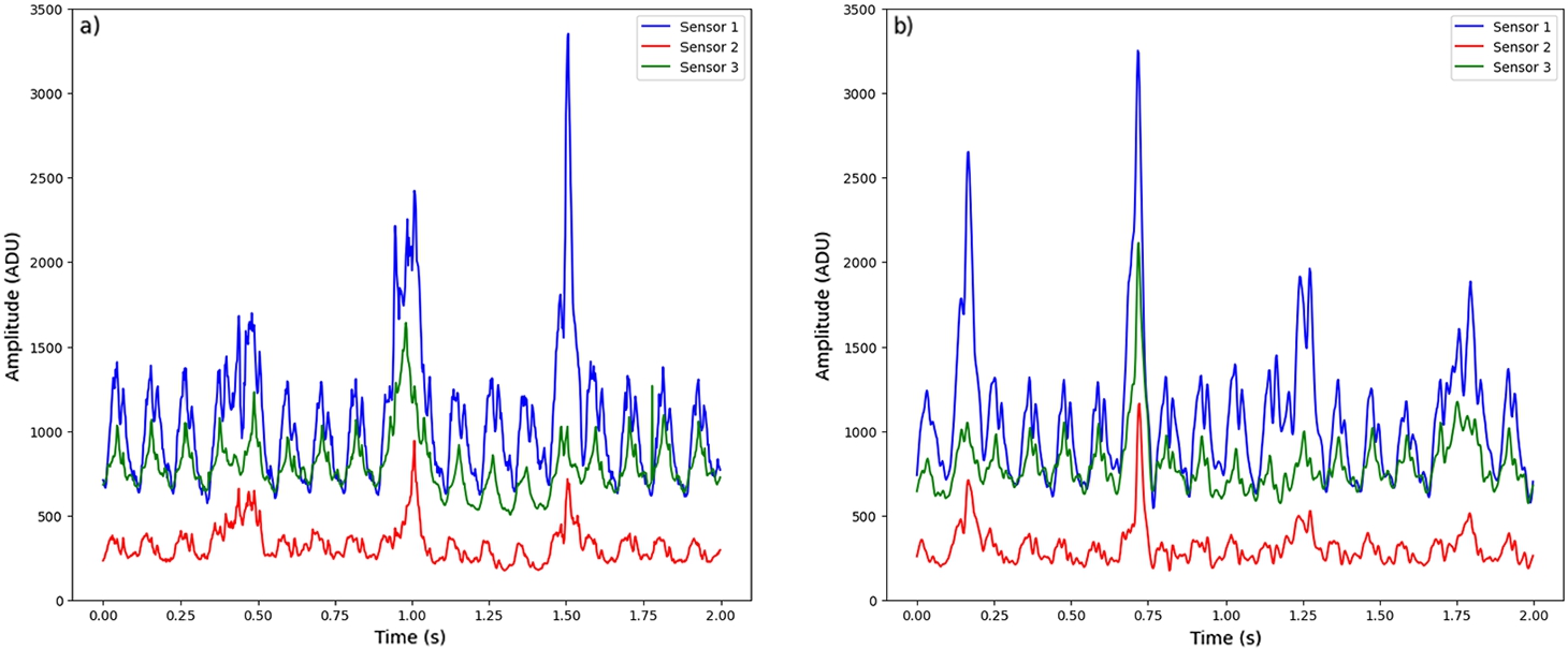
A comparison of original and randomly generated signal is presented in Fig. 14. It can be seen that the amplitude and frequency of the generated signal are similar to that of the real signal, but the generated signal has less noise.

Fig. 14

CB tension signals: a) original signal; b) TimeVAE generated signal.

3.2Classification Accuracy Study

The study on the classification accuracy of CB states was carried out in two stages. In the first stage, different DNN models were assessed by classifying the signals processed by a sliding window of varying lengths (0.5 s, 1.0 s, 1.5 s, 2.0 s) without applying any additional data augmentation methods. The second stage focused on examining the impact of different data augmentation methods on the classification accuracy of DNN models, specifically using 2.0 s-length signals. The 2.0 s-length signals were selected for this stage because their dataset was the smallest.

3.2.1DNN Models’ Study

For each signal length (0.5 s, 1.0 s, 1.5 s, 2.0 s), the CB dataset was divided into five parts, ensuring class balance in each fold. Balanced 5-fold cross-validation was used to construct the training and testing sets. This approach involved using 80% of the data (four out of five folds) for training and 20% (the remaining fold) for testing. Training and testing sets were switched five times for each signal length. The final accuracy was calculated by averaging the results of these five training runs and determining the standard error of the mean. This method was chosen to provide a more reliable estimate of the model classification accuracy, particularly given the small dataset sizes.

Table 2

Augmentation-free multi-class (0.5 kg, 1 kg, 2 kg, 3 kg, 5 kg, and a class for a damaged belt) classification accuracy of CB states of DNN models.

Signal length, s	Accuracy ± SE, %
Signal length, s	CNN-LSTM	FCN	ResNet	InceptionTime
0.5	74.3±0.82	76.4±1.14	80.6±1.27	79.3±0.71
1.0	65.5±1.08	81.5±1.29	85.4±1.26	84.9±0.59
1.5	66.3±2.47	83.7±1.51	84.8±1.09	84.8±1.52
2.0	64.3±1.58	88.1±1.48	91.1±1.09	89.1±1.54

A total of 6 different classes were assigned to the tension signals based on their load and defect states: 0.5 kg, 1 kg, 2 kg, 3 kg, 5 kg, and a class for a belt with damage. A categorical cross-entropy loss function was used for all classification models, with a softmax activation function applied to the output layer. Each model was trained five times for 300 epochs per experiment, using a batch size of 16 signals per iteration. Before training, all training sets of different lengths were aligned to ensure that each set consisted of 2000 signals. To achieve this, the training sets in the first stage were multiplied without augmentations to reach the required 2000 signals.

The classification accuracy results of CB states in the first stage, using various DNN models without augmentations, are presented in Table 2. According to the results, ResNet model outperformed other models in all signal lengths and had the highest classification accuracy, which reached 91.1%±1.09% with 2.0 s-length signals. ResNet and InceptionTime models have demonstrated similar accuracies for all the signal lengths, differing by only one or two percentage points. FCN model also performed competitively, achieving an accuracy of 88.1%±1.48% with 2.0 s-length signals, which was only slightly lower than that of ResNet and InceptionTime models. The accuracy of CNN-LSTM model decreased in line with increasing signal length, indicating that it performed comparatively poorly for this classification task. In addition, the accuracy of all other models improved with increasing signal length, except of CNN-LSTM model.

Table 3

Augmentation-free multi-class (0.5 kg, 1 kg, 2 kg, 3 kg, 5 kg, and a class for a damaged belt) classification recall of CB states of DNN models for each class.

Model	Signal length, s	Recall, %
Model	Signal length, s	0.5 kg	1 kg	2 kg	3 kg	5 kg	With damage
CNN-LSTM	0.5	71.6	61.0	51.6	64.2	74.3	98.2
	1.0	59.8	28.6	42.8	65.5	69.4	96.8
	1.5	69.4	38.0	47.2	58.6	66.3	94.0
	2.0	60.8	43.4	43.6	57.0	66.9	96.8
FCN	0.5	77.2	62.6	56.2	64.8	76.4	98.6
	1.0	78.8	84.0	51.6	76.0	81.5	100
	1.5	95.6	64.4	69.4	72.4	81.6	97.6
	2.0	96.6	80.0	70.0	88.8	90.4	98.4
ResNet	0.5	83.8	72.6	55.6	73.2	80.6	99.2
	1.0	91.6	75.4	61.0	85.2	85.4	100
	1.5	88.4	75.2	67.6	81.6	85.9	100
	2.0	100	79.0	72.2	91.1	97.2	100
InceptionTime	0.5	85.8	64.4	57.8	69.4	79.3	99.2
	1.0	88.6	82.6	64.6	74.6	84.9	100
	1.5	93.2	68.3	75.0	82.0	84.8	100
	2.0	93.4	85.0	66.2	90.1	91.6	100

Table 4

Augmentation-free multi-class (0.5 kg, 1 kg, 2 kg, 3 kg, 5 kg, and a class for a damaged belt) classification precision of CB states of DNN models for each class.

Model	Signal length, s	Precision, %
Model	Signal length, s	0.5 kg	1 kg	2 kg	3 kg	5 kg	With damage
CNN-LSTM	0.5	66.4	55.0	53.8	74.8	75.0	98.8
	1.0	49.6	32.2	48.0	66.4	72.4	98.0
	1.5	59.4	44.6	39.4	65.8	67.5	100
	2.0	51.8	40.6	41.8	66.3	68.6	100
FCN	0.5	67.6	63.8	56.6	72.6	76.7	99.0
	1.0	77.2	66.0	67.0	83.2	88.8	100
	1.5	77.2	78.2	69.4	84.0	90.2	100
	2.0	87.0	79.4	83.8	88.1	95.0	98.6
ResNet	0.5	73.8	71.8	66.8	73.6	80.8	98.4
	1.0	80.2	75.0	72.6	85.4	85.5	100
	1.5	77.6	70.2	76.8	85.9	92.0	100
	2.0	97.2	83.8	78.4	91.7	93.2	100
InceptionTime	0.5	69.6	73.0	62.6	72.0	79.6	99.6
	1.0	77.8	86.2	67.2	82.2	85.5	100
	1.5	73.6	81.8	74.5	85.6	94.0	100
	2.0	95.6	71.6	78.6	89.1	97.2	100

Table 5

Augmentation-free multi-class (0.5 kg, 1 kg, 2 kg, 3 kg, 5 kg, and a class for a damaged belt) classification F1-score of CB states of DNN models for each class.

Model	Signal length, s	F1-score, %
Model	Signal length, s	0.5 kg	1 kg	2 kg	3 kg	5 kg	With damage
CNN-LSTM	0.5	68.6	57.6	52.6	68.6	74.3	98.6
	1.0	53.6	29.8	45.0	65.6	70.8	97.2
	1.5	63.4	39.8	42.2	61.0	66.1	97.0
	2.0	55.0	41.2	41.8	62.2	65.9	98.4
FCN	0.5	71.8	63.0	56.0	68.6	76.2	98.6
	1.0	76.4	72.4	58.2	80.8	81.3	100
	1.5	84.6	69.8	68.6	84.2	85.0	98.8
	2.0	90.8	78.2	73.2	88.1	91.2	98.6
ResNet	0.5	77.8	71.8	60.2	73.0	80.2	98.8
	1.0	85.6	75.0	65.6	84.6	85.0	100
	1.5	82.2	72.0	70.2	84.6	86.0	100
	2.0	98.4	80.4	73.6	90.8	94.6	100
InceptionTime	0.5	76.6	68.0	59.8	70.8	79.1	99.4
	1.0	82.2	83.2	64.0	78.2	84.5	100
	1.5	81.6	73.8	74.2	84.5	87.2	100
	2.0	93.6	77.2	71.6	89.1	94.0	100

The results of classification recall, precision, and F1 statistics for all the models of CB states for each class are presented in Tables 3, 4, and 5. The results show that all the models classified the damaged CB class with the highest accuracy, for example, F1 statistics of ResNet and InceptionTime models for 1.0 s, 1.5 s and 2.0 s signals reached 100% accuracy for this class. Different load states were classified worse by all the models. All the models were the most sensitive to 0.5 kg, 5 kg, and damaged-belt states, possibly because these signals stood out the most, while the 1 kg, 2 kg, and 3 kg signals were relatively similar, bringing more difficulty in their classification.

The training times of DNN models for various CB signal lengths are presented in Table 6. The signal length refers to the duration of the input CB signal (in seconds), and the epoch training time is the time (in seconds) taken by each model to complete one training epoch. The table shows that FCN model required the shortest training time for all the signal lengths. Meanwhile, ResNet and InceptionTime models took the longest training time. For example, for 2.0 s signals, training time of ResNet was 3.4 s and that of InceptionTime 3.6 s, while that of FCN took 0.8 s only. On the average, training time of InceptionTime model took several fractions of a second longer than that of ResNet, making it the slowest to train of all the studied models. Longer training time of ResNet and InceptionTime models likely occurred due to larger number of their parameters.

Table 6

Single epoch training time of DNN models.

Signal length, s	Epoch training time, s
Signal length, s	CNN-LSTM	FCN	ResNet	InceptionTime
0.5	0.6	0.3	0.7	0.9
1.0	1.0	0.5	1.8	2.1
1.5	1.2	0.7	2.8	2.7
2.0	1.5	0.8	3.4	3.6

The first-stage study demonstrated that without any data augmentations, ResNet model was the most accurate for CB state classification. Also, FCN model’s classification accuracy was only slightly lower than that of ResNet and InceptionTime models. FCN model had the advantage of being the fastest to train and requiring fewer computing resources as compared to other models. The next stage of the research explores the impact of various data augmentation methods on the classification accuracy of DNN models by artificially augmenting CB signal dataset.

3.2.2Data Augmentation Impact

In the second stage of the research, a study of data augmentation methods was carried out with the purpose of comparing the impact of various augmentation methods on DNN models in the classification of CB states. The study used the 2.0 s sliding-window processed signals because this dataset was the smallest, consisting of only 233 signals.

A balanced 5-fold cross-validation was also used for each experiment. The hyperparameters for training the models were the same as in the first stage, that is, in each experiment, the models were trained 5 times for 300 epochs, where the batch size of one iteration was 16 signals. However, at this stage, various data augmentations were applied to artificially increase the training sets, increasing the size of each of them to 2000 signals.

Table 7

Multi-class (0.5 kg, 1 kg, 2 kg, 3 kg, 5 kg, and a class for a damaged belt) classification accuracy for all used augmentation methods.

Augmentation method	Accuracy ± SE, %
Augmentation method	CNN-LSTM	FCN	ResNet	InceptionTime
No augmentations	64.3±1.58	88.1±1.48	91.1±1.09	89.1±1.54
Laplace (std/100)	62.4±4.00	89.1±1.35	91.6±1.08	92.1±1.32
Laplace (std/50)	61.4±1.71	89.6±1.91	91.1±0.90	90.6±1.12
Laplace (std/20)	59.9±1.68	91.1±1.11	91.6±0.86	92.4±0.72
Drifted Gaussian (std/100)	61.9±3.04	91.1±1.82	90.1±0.71	91.1±1.68
Drifted Gaussian (std/50)	64.4±1.54	88.1±2.87	92.1±1.47	91.6±1.14
Drifted Gaussian (std/20)	61.9±1.61	92.5±1.86	90.1±0.94	89.5±1.08
Uniform (std/100)	62.9±2.20	89.1±1.91	90.1±1.44	91.1±1.09
Uniform (std/50)	59.9±1.30	89.6±1.27	91.1±1.14	90.6±0.47
Uniform (std/20)	59.9±2.71	89.1±1.49	89.1±1.54	89.2±2.09
Laplace and drifted Gaussian	63.4±2.56	92.6±1.54	91.1±0.92	90.6±0.85
Laplace and uniform noise	62.9±1.97	89.1±1.51	91.1±0.87	92.5±0.71
Magnitude warping	59.4±2.13	88.1±1.93	90.6±2.19	90.1±1.41
TimeVAE	75.7±0.88	77.2±2.75	90.1±2.93	88.6±2.90

The classification accuracy results of each experiment for all DNN models using various data augmentations are presented in Table 7. The results also show the baseline classification accuracy of each model without augmentations, which were obtained in the first phase of the study by classifying 2.0 s-length signals.

The results show that each data augmentation affected the classification accuracy differently, depending on the model and the augmentation method itself. The best classification accuracy results after applying data augmentations were achieved by using FCN, ResNet, and InceptionTime models.

Adding Laplace noise increased the accuracy of FCN, ResNet, and InceptionTime models across all the noise levels, but decreased the accuracy of CNN-LSTM model. The addition of drifted Gaussian noise notably increased the baseline classification accuracy of FCN model by 4.4% to 92.5%±1.86% with std/20 noise. It also increased the accuracy of ResNet model with std/50 noise by 1% to 92.1%±1.47%, and InceptionTime model by 2% to 91.1%±1.68% with std/100 noise. Adding uniform noise resulted on the average in worse classification results for all the models as compared to adding Laplace or drifted Gaussian noise.

The best accuracy result of the entire study, which increased the baseline accuracy of FCN model by 4.5% to 92.6%±1.54%, was achieved by training the model on data augmented with combined Laplace and drifted Gaussian noise. Adding Laplace and uniform noise increased the accuracy of InceptionTime model by 3.4% to 92.5%±0.71%. All the experiments involving combined noise used noise with a size of std/100.

Magnitude warping augmented data increased the accuracy of only InceptionTime model by 1% to 90.1%±1.41%. Augmenting signals with TimeVAE increased the accuracy of only CNN-LSTM model, which reached 75.7%±0.71%, but was still lower as compared to other models.

CNN-LSTM model generally experienced a negative impact from most data augmentations, except for TimeVAE-generated signals, which had a positive effect. Most data augmentations improved the baseline accuracy of FCN model, although TimeVAE augmentation led to a decrease of 10.9%. For ResNet model, most augmentations either reduced the accuracy or resulted in only a marginal improvement of 1%.

Fig. 15

Comparison of change in classification accuracy of data augmentation methods for each model with baseline (no augmentation) accuracy. Accuracy changes of: a) CNN-LSTM; b) FCN; c) ResNet; d) InceptionTime.

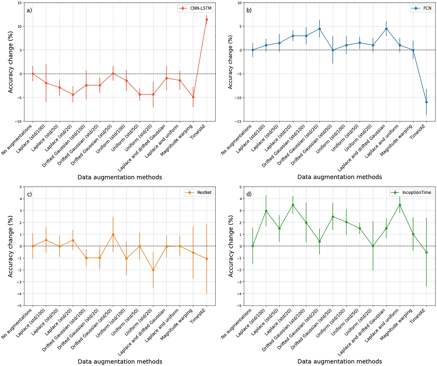
The changes in classification accuracy of each model achieved by various data augmentation methods are presented in Fig. 15. Separate graphs show the relative change in accuracy for each model as compared to baseline (without any augmentation) accuracy. CNN-LSTM model generally experienced a negative impact from most data augmentations, except for TimeVAE-generated signals, which had a positive effect. Most data augmentations improved the baseline accuracy of FCN model, although TimeVAE augmentation led to a decrease of 10.9%. For ResNet model, most augmentations either reduced accuracy or resulted in only a marginal improvement of 1%. The baseline classification accuracy of InceptionTime model was increased by almost all the data augmentations.

The plot analysis revealed that for FCN and InceptionTime models, almost all the data augmentation methods increased the baseline classification accuracy. However, for ResNet and CNN-LSTM models, most augmentations had a negative impact on the classification accuracy. Likely, the architecture of FCN and InceptionTime models allowed them to adapt more effectively to specific augmentation methods, thereby enhancing their overall classification accuracy and robustness.

The results of the second stage of the study showed that FCN model trained with augmented data classified CB load and defect states with an accuracy of 92.6%±1.54%. This model was comparable to ResNet and InceptionTime models in terms of classification accuracy, but FCN model was trained much faster due to its small number of trainable parameters. ResNet model achieved an accuracy of 92.1%±1.47% with data augmented by drifted Gaussian noise, while InceptionTime model achieved its best result of 92.5%±0.71% with data augmented by random Laplace and uniform noise. CNN-LSTM model achieved its highest accuracy of 75.7%±0.88% when trained with signals generated by TimeVAE model. The best accuracy results of FCN, ResNet, and InceptionTime models were very similar and differed only slightly, but the accuracy of CNN-LSTM model was much worse.

4Conclusion

In this research, we examined existing DL algorithms and DNN architectures for classifying CB states. In addition, various time series data augmentation methods applicable to CB tension signals were examined.

The study successfully developed and evaluated several DNN models for the classification of CB load and defect states using tension signals, specifically based on FCN, ResNet, InceptionTime, and CNN-LSTM architectures. FCN model was able to classify CB states with an accuracy of 92.6%±1.54%, making it the most accurate of the studied models. ResNet and InceptionTime models also performed well, with accuracies of 92.1%±1.47% and 92.5%±0.71%, respectively. CNN-LSTM model demonstrated the worst results, with a maximum accuracy of 75.7%±0.88% only.

The impact of various data augmentation methods on classification accuracy was also analysed. The combined addition of Laplace and drifted Gaussian noise increased the baseline (without any augmentation) accuracy of FCN model by 4.5% to 92.6%±1.54%. Adding Laplace and uniform noise increased the accuracy of InceptionTime model by 3.4% to 92.5%±0.71%. The classification accuracy of CNN-LSTM model trained with signals generated by TimeVAE increased by 11.4% to 75.7%±0.88%, but it still remained much lower than that of other models. The baseline accuracy of ResNet model increased by 1% only to 92.1%±1.47% after training with drifted Gaussian noise augmented data.

These results underline the effectiveness of applying data augmentations to small CB tension signal datasets, enhancing the classification accuracy of models based on FCN and InceptionTime architectures. In classifying CB states, FCN-based model showed higher accuracy and speed compared to other models, despite having the lowest amount of trainable parameters. Successful application of FCN model demonstrated the importance of selecting and optimizing the right architecture for specific data and classification tasks.

CB status classification under fixed loads and rotation speed could be considered as a limitation of this study. A set of fixed parameters does not reflect real world conditions and future investigations should be based on random CB status classification on unseen experiment parameters. Empirical model parameters selection method can be also considered a limitation of this study.

Further research on CB state classification could aim to improve accuracy in classifying weights of similar mass (1 kg, 2 kg, 3 kg). Additionally, future research could explore advanced generative data augmentation techniques, for example, those utilizing GANs or other VAE architectures to enhance the quality of CB tension signal data.

Notes

1 https://github.com/ArmantasPik/Conveyor-belt-state-classification/

Acknowledgements

This paper has received funding under postdoctoral fellowship project from the Research Council of Lithuania (LMTLT), agreement No. [S-PD-22-81].

References

1	Andrejiova, M., Grincova, A., Marasova, D. ((2021) ). Identification with machine learning techniques of a classification model for the degree of damage to rubber-textile conveyor belts with the aim to achieve sustainability. Engineering Failure Analysis, 127: , 105564.
2	Bortnowski, P., Król, R., Ozdoba, M. ((2022) a). Roller damage detection method based on the measurement of transverse vibrations of the conveyor belt. Eksploatacja i Niezawodność, 24: (3), 510–521.
3	Bortnowski, P., Kawalec, W., Król, R., Ozdoba, M. ((2022) b). Types and causes of damage to the conveyor belt–review, classification and mutual relations. Engineering Failure Analysis, 140: , 106520.
4	Chlap, P., Min, H., Vandenberg, N., Dowling, J.A., Holloway, L., Haworth, A. ((2021) ). A review of medical image data augmentation techniques for deep learning applications. Journal of Medical Imaging and Radiation Oncology, 65: (5), 545–563.
5	Dąbek, P., Wróblewski, A., Wodecki, J., Bortnowski, P., Ozdoba, M., Król, R., Zimroz, R. ((2023) ). Application of the methods of monitoring and detecting the belt mistracking in laboratory conditions. Applied Sciences, 13: (4), 2111.
6	Desai, A., Freeman, C., Wang, Z., Beaver, I. (2021). Timevae: a variational auto-encoder for multivariate time series generation. arXiv preprint arXiv:2111.08095.
7	Goodfellow, I., Pouget-Abadie, J., Mirza, M., Xu, B., Warde-Farley, D., Ozair, S., Courville, A., Bengio, Y. (2014). Generative adversarial nets. Advances in Neural Information Processing Systems, 27.
8	Goubeaud, M., Joußen, P., Gmyrek, N., Ghorban, F., Schelkes, L., Kummert, A. (2021). Using Variational Autoencoder to augment Sparse Time series Datasets. In: 2021 7th International Conference on Optimization and Applications (ICOA), pp. 1–6.
9	Gregor Hartmann, K., Tibor Schirrmeister, R., Ball, T. (2018). EEG-GAN: Generative adversarial networks for electroencephalograhic (EEG) brain signals. arXiv e-prints, arXiv:1806.01875v1.
10	Hsiao, T.-Y., Chang, Y.-C., Chou, H.-H., Chiu, C.-T. ((2019) ). Filter-based deep-compression with global average pooling for convolutional networks. Journal of Systems Architecture, 95: , 9–18.
11	Huang, T., Chakraborty, P., Sharma, A. ((2023) ). Deep convolutional generative adversarial networks for traffic data imputation encoding time series as images. International Journal of Transportation Science and Technology, 12: (1), 1–18.
12	Iglesias, G., Talavera, E., González-Prieto, Á., Mozo, A., Gómez-Canaval, S. ((2023) ). Data augmentation techniques in time series domain: a survey and taxonomy. Neural Computing and Applications, 35: (14), 10123–10145.
13	Iwana, B.K., Uchida, S. ((2021) ). Time series data augmentation for neural networks by time warping with a discriminative teacher. In: 2020 25th International Conference on Pattern Recognition (ICPR). IEEE, pp. 3558–3565.
14	Kingma, D.P., Welling, M. ((2019) ). An introduction to variational autoencoders. Foundations and Trends® in Machine Learning, 12: (4), 307–392.
15	Klištincová, N., Pin, L., Puškárová, A., Giannino, D., Bučková, M., Lambreva, M.D., Manfredini, A., Canfora, L., Pangallo, D., Pinzari, F. ((2024) ). From farm to fork: fungal and bacterial contaminants and their diagnostics in the production steps of ready-to-eat salads. Trends in Food Science & Technology, 150: , 104573.
16	Li, X.-G., Miao, C.-Y., Wang, J., Zhang, Y. ((2011) ). Automatic defect detection method for the steel cord conveyor belt based on its X-ray images. In: 2011 International Conference on Control, Automation and Systems Engineering (CASE), pp. 1–4.
17	Long, J., Shelhamer, E., Darrell, T. ((2015) ). Fully convolutional networks for semantic segmentation. In: Proceedings of the IEEE Conference on Computer Vision and Pattern Recognition, pp. 3431–3440.
18	Santos, A.A., Rocha, F.A., Reis, A.J.d.R., Guimarães, F.G. ((2020) ). Automatic system for visual detection of dirt buildup on conveyor belts using convolutional neural networks. Sensors, 20: (20), 5762.
19	Sarker, I.H. ((2021) ). Deep learning: a comprehensive overview on techniques, taxonomy, applications and research directions. SN Computer Science, 2: , 420.
20	Smith, K.E., Smith, A.O. (2020). Conditional GAN for timeseries generation. arXiv preprint arXiv:2006.16477.
21	Um, T.T., Pfister, F.M., Pichler, D., Endo, S., Lang, M., Hirche, S., Fietzek, U., Kulić, D. ((2017) ). Data augmentation of wearable sensor data for Parkinson’s disease monitoring using convolutional neural networks. In: Proceedings of the 19th ACM International Conference on Multimodal Interaction, pp. 216–220.
22	Wang, J., Perez, L. ((2017) a). The effectiveness of data augmentation in image classification using deep learning. Convolutional Neural Networks Vis. Recognit, 11: (2017), 1–8.
23	Wang, Y., Miao, C., Miao, D., Yang, D., Zheng, Y. ((2023) ). Hazard source detection of longitudinal tearing of conveyor belt based on deep learning. PLoS ONE, 18: (4), 0283878.
24	Wang, Z., Yan, W., Oates, T. ((2017) b). Time series classification from scratch with deep neural networks: a strong baseline. In: 2017 International Joint Conference on Neural Networks (IJCNN). IEEE, pp. 1578–1585.
25	Yoon, J., Jarrett, D., Van der Schaar, M. (2019). Time-series generative adversarial networks. Advances in Neural Information Processing Systems, 32.
26	Zhang, M., Shi, H., Zhang, Y., Yu, Y., Zhou, M. ((2021) ). Deep learning-based damage detection of mining conveyor belt. Measurement, 175: , 109130.
27	Žvirblis, T., Petkevičius, L., Bzinkowski, D., Vaitkus, D., Vaitkus, P., Rucki, M., Kilikevičius, A. ((2022) ). Investigation of deep learning models on identification of minimum signal length for precise classification of conveyor rubber belt loads. Advances in Mechanical Engineering, 14: (6), 1–13.