
ALMERIA: Boosting Pairwise Molecular Contrasts with Scalable Methods
Abstract
This work introduces ALMERIA, a decision-support tool for drug discovery. It estimates compound similarities and predicts activity, considering conformation variability. The methodology spans from data preparation to model selection and optimization. Implemented using scalable software, it handles large data volumes swiftly. Experiments were conducted on a distributed computer cluster using the DUD-E database. Models were evaluated on different data partitions to assess generalization ability with new compounds. The tool demonstrates excellent performance in molecular activity prediction (ROC AUC: 0.99, 0.96, 0.87), indicating good generalization properties of the chosen data representation and modelling. Molecular conformation sensitivity is also evaluated.
1Introduction
Finding a lead compound that can be optimized to result in a drug candidate is an arduous task that entails high costs both in terms of time and funds, mainly because of the vast chemical space. For that reason, computational methods are employed to select a smaller subset of potentially promising compounds for biological testing. This process is known as virtual screening. It comprehends different methods depending on the amount of available information about the compounds in a given database and the biological reactions from previous assays with one of the query compounds or between potentially similar compounds. For instance, the simplest approach regarding the amount of utilized prior information is based on the similarity of the compounds. Molecular similarity (Maggiora et al., 2014) could be measured from different perspectives. However, the basic assumption is that structurally similar molecules tend to have similar properties, although this deduction is only sometimes completely evident (Martin et al., 2002). Moreover, such similarities can be a potential subject of what is known as activity cliff (Hu and Bajorath, 2020), i.e. a small modification to a functional group leads to a sudden change in activity. As aforementioned, molecular similarity can be measured from different perspectives that include the distance11 between molecular descriptors or fingerprints (Cereto-Massagué et al., 2015), or alignment-based 3-D similarity, which takes into account rotations and conformations, such as shape similarity (Kumar and Zhang, 2018; Puertas-Martín et al., 2019), among others. The last few years have seen the widespread adoption of deep learning for different problem domains, especially for problems involving unstructured data such as text or images. Deep learning approaches have also been applied for similarity by letting them learn a feature representation in the network latent space. These approaches include neural machine translation (Winter et al., 2019; Xu et al., 2017) and language models (Li and Jiang, 2021) for string-based representations such as SMILES, variational autoencoders also with SMILES representation (Samanta et al., 2020), or contrastive learning using graph representations (Wang et al., 2022). The main benefit of these approaches is also their main drawback, as they use unlabelled data and perform data augmentation (atom masking, bond deletion, and subgraph removal) for a given molecule. However, they require labelled data for fine-tuning the last layers in the model in order to achieve a competent performance in downstream tasks.
Another approach is to leverage the available information on known active and inactive compounds to build a predictive model. Input data may also vary from numerical molecular descriptors, the molecular structure in graph notation, and image or string-based representations. Whatever the case, the aim is to find a function mapping from such input space into the output space related to the biological activity between the compounds, for instance. Historically, a reduced number of numerical properties were used in order to quantitatively express their influence on the response variable, which is known as Quantitative-Structure Activity Relationships (QSAR) (Cherkasov et al., 2014) where descriptor selection is fundamental to discard those irrelevant ones beforehand (Shahlaei, 2013; Martínez et al., 2019). Later, methods based on machine learning that were able to handle larger volumes of data were used for that purpose (Mao et al., 2021) and in a more automated manner. It includes approaches such as convolutional neural networks (Stepniewska-Dziubinska et al., 2018; Jiménez et al., 2018; Ruiz Puentes et al., 2021), graph networks with attention (Cheng et al., 2021; Hung and Gini, 2021; Yin et al., 2021), or gradient boosting applied with a learning-to-rank procedure (Furui and Ohue, 2022), among others. The main problem with these approaches is precisely the use of annotated data, which is scarce compared to the entire chemical space and expensive to obtain for new pairs of compounds. That is the entire goal of virtual screening: to reduce the potential search space while reducing the risk of omitting promising compounds. Another related problem is derived from the small explored chemical space and the optimization procedures to fit such data that could reward memorization instead of the sought-after generalization for new unseen compounds (Wallach and Heifets, 2018).
Lastly, when the 3-D structure of the target molecule is known, structure-based methods such as molecular docking may be applied. However, the space of target molecules with known structures is small compared to the entire space. Additionally, these methods are sensitive to the orientation and torsion of the molecule conformations, but especially to the scoring function (Plewczynski et al., 2011; Shen et al., 2021).
For a more in depth overview on the literature on virtual screening, the interested reader is referred to a diverse collection of references such as Kimber et al. (2021), Deng et al. (2021), Jiang et al. (2021), Banegas-Luna et al. (2018).
The present work could be framed as a structure-activity relationship (SAR) model but leveraging large-scale high-dimensional data. We put the focus on designing a curated methodology to characterize the molecules in a given database, which comprehends both the modelling of the molecule with different conformations to have a richer 3-D perspective and the generation of nearly 5000 molecular descriptors for every molecule conformation. The choice of using numerical descriptors from the 3-D representations instead of the 3-D representations themselves as images, for instance, is because we consider the former an unbiased representation. It is more easily manageable by algorithms, less noisy, and more likely to have less impact on the time to diagnose and interpret a result. A simple example is that of a group of pixels against certain numerical features of the molecular structure. The work presented here is based on a supervised learning approach to make the most of the activity annotated data, being the ability to generalize with new compounds the ultimate goal of this work. Moreover, this proposal relies on artificial intelligence methods to exploit high-dimensional data instead of over-optimizing based on a specific criterion (e.g. shape).
The contribution of this research lies in the development of the decision-support tool ALMERIA. This tool enables the estimation of compound similarities and activity predictions by leveraging pairwise molecular contrasts, while also accounting for conformational variability. Here are the key aspects of its contribution:
1. Data Augmentation: ALMERIA employs pairwise molecular contrasts as a form of data augmentation. By considering variations in molecular conformations, it enhances the accuracy of predictions.
2. Scalability: The methodology has been implemented using scalable software and methods, allowing it to handle large volumes of data (up to several terabytes). Even when processing a substantial batch of queries, ALMERIA provides rapid responses.
3. Model Evaluation: Detailed data split criteria have been applied to evaluate the models on different data partitions. This rigorous evaluation ensures that the models generalize well to new compounds.
4. State-of-the-Art Performance: Experimental results demonstrate state-of-the-art performance in molecular activity prediction, with noteworthy ROC AUC values of 0.99, 0.96, and 0.87.
5. Robustness and Generalization: The chosen data representation and modelling techniques exhibit good properties for generalization. Additionally, sensitivity analysis of molecular conformations further validates the robustness of ALMERIA’s predictions.
In summary, ALMERIA contributes significantly to efficient drug discovery pipelines by providing accurate predictions and narrowing down the search space for potential active compounds. Its robustness and scalability make it a valuable tool in modern cheminformatics research.
The document is structured as follows: Section 2 describes the proposed materials and methods using a generic and modular architecture, while the specific implementation details, as well as the obtained results, are discussed in Section 3. Some performance measurements – both in CPU and GPU – are given in Section 4. Finally, in Section 5, conclusions and potential future work are drawn.
2Materials and Methods
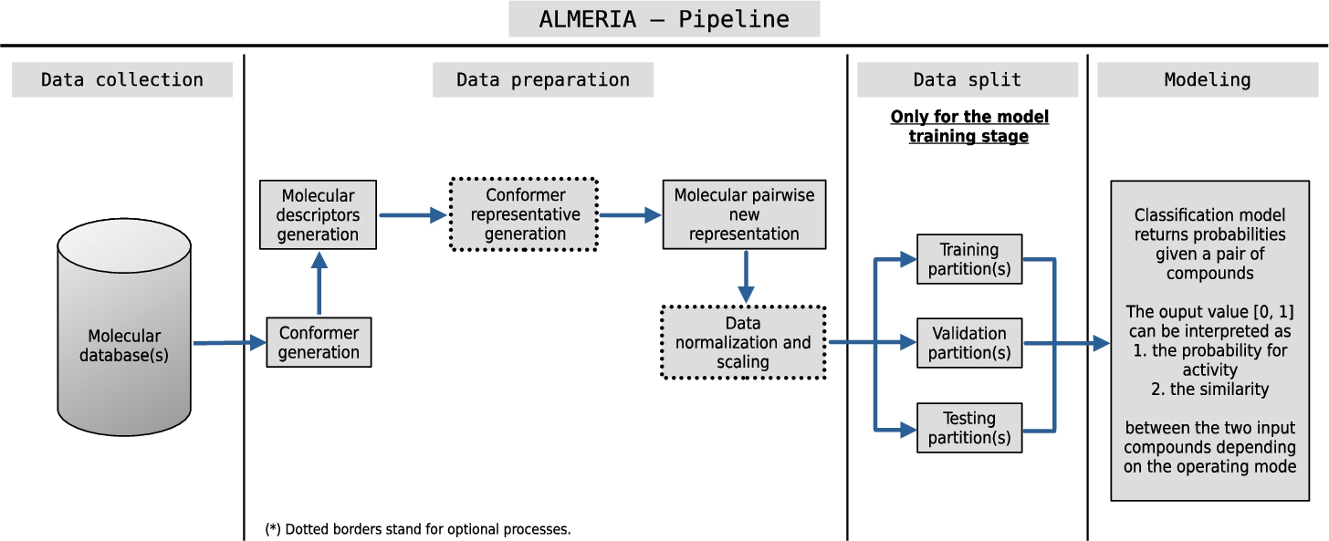
The general scheme showing the flow of information using the proposed materials and methods can be seen in Fig. 1. The boxes in the diagram intentionally show generic names for the proposed materials and methods, intending to modularise the methodology and reflect the flexibility to replace specific portions of the proposal. In this section, the functionality covered in each part will be described briefly and from a fundamental point of view. However, it will be in Section 3.1 where more details on the specific implementation for this work will be given.
Fig. 1
Overall scheme for ALMERIA using the proposed materials and methods. The data pipeline begins by collecting data from molecular databases and subsequently prepares it for further use. This data preparation includes generating molecular descriptors and conformer representative generation, which might involve creating new representations of the molecules. Next, the data is split into partitions for training, validation, and testing. The training partition is used to build the classification model, which takes a pair of compounds as input and outputs a probability value between 0 and 1. This value can be interpreted as a probability of activity or similarity between the two compounds, depending on the model’s operating mode. Validation partition is usually coupled within a cross-validation schema. Finally, testing partition is not used during training, but to assess the out-of-sample performance of the final.
2.1Data Collection
Any molecular database could be used to feed the pipeline shown in Fig. 1. The only requisite for the model training stage is to have a certain number of active compounds. These compounds can come from a labeled dataset, where each compound is given a binary label indicating whether it is active or inactive. Of course, this requirement does not apply to the prediction mode as the final aim is to predict the potential biological activity between new molecules. ALMERIA has therefore been designed to make the most of the already activity-labelled data; it is not necessary to have the entire database(s) already labelled with the biological activity, but a subset may suffice. However, as always with data-driven models, the more and better quality data, the more likely it is that a good, generalizable model will be obtained.
Table 1
Number of molecular descriptors grouped by logical block using Dragon software.
| Block name | Number of descriptors |
| Constitutional descriptors | 43 |
| Ring descriptors | 32 |
| Topological indices | 75 |
| Walk and path counts | 46 |
| Connectivity indices | 37 |
| Information indices | 48 |
| 2D matrix-based descriptors | 550 |
| 2D autocorrelations | 213 |
| Burden eigenvalues | 96 |
| P-VSA-like descriptors | 45 |
| ETA indices | 23 |
| Edge adjacency indices | 324 |
| Geometrical descriptors | 38 |
| 3D matrix-based descriptors | 90 |
| 3D autocorrelations | 80 |
| Block name | Number of descriptors |
| RDF descriptors | 210 |
| 3D-MoRSE descriptors | 224 |
| WHIM descriptors | 114 |
| GETAWAY descriptors | 273 |
| Randic molecular profiles | 41 |
| Functional group counts | 154 |
| Atom-centered fragments | 115 |
| Atom-type E-state indices | 170 |
| CATS 2D | 150 |
| 2D Atom Pairs | |
| 3D Atom Pairs | 36 |
| Charge descriptors | 15 |
| Molecular properties | 20 |
| Drug-like indices | 27 |
In contrast, the size and dimensionality of the molecular database(s) are not restricted because the methodology and implementation details have been chosen carefully to be scalable. These include using big data-oriented software such as Dask (Dask Development Team, 2016), allowing the entire pipeline operations to be executed in parallel and distributed over a cluster of computers.
As the molecules in the database are given in a rigid state, we use the software OpenEye Scientific Omega (Hawkins et al., 2010) to generate a set of 3-D molecular conformations for every compound in the database. That way, we have a broader representation of a molecule’s different conformations. However, care must be taken as the number of conformations for a given molecule may suffer from a combinatorial explosion. If each torsion angle is rotated in increments of θ degrees for a molecule with N rotatable bonds, then the total number of conformations would be
Next, we use these molecular conformations to generate a large set of
2.2Data Preparation
Once data is collected, we have decided not to perform any major data transformation or dimensionality reduction along the descriptors’ axis to avoid harming the interpretability of the model. However, we opted for performing two preprocessing steps to both favour the method generalization and make the process more efficient:
1. The set of conformations for every compound is reduced to a single representative sample by averaging their descriptor values, i.e. grouping by molecule and then averaging their descriptors column-wise. Thus, this representative sample is built considering the different conformations the molecule may adopt. As a side effect, this improves the efficiency of model building. The first benefit sought with this step is fairer when guiding the model optimization and evaluating its performance, as activity data is usually molecule-wise labelled. However, conformation generation may imply that certain molecules are overrepresented in comparison to others, which may bias both the optimization and the evaluation metrics, i.e. risk of frequency bias. In any case, this step is optional for ALMERIA within the proposed methodology shown in Fig. 1, and all conformations could be used for modelling. However, since we have included this step in the current work and know that it can be controversial outside the field of machine learning, we have included Section 3.4 within the experimentation that analyses its impact on the set of generated conformations.
2. Instead of building a separate model for every target, as often found in literature, we opt for building a single model that considers the specific contrast between compounds that correlates with biological activity. We achieve this by performing the absolute difference on the descriptors for every pair of target and ligand molecules. This procedure has a data augmentation effect, and it aims to improve the generalization performance with compounds not yet seen during the model fitting while making the ALMERIA methodology more efficient with a single model without sacrificing interpretability.
2.3Data Split
In addition to the previous data modelling choices, we have also been careful during the model-building stage to make the most efficient use of the available data and to maximize the generalization. Given that we are adopting a supervised learning approach, we have considered that such labelled data is expensive to obtain. This consideration is important, as it is well known that poorly trained machine learning models can easily over-fit the training data and perform much worse with new and potentially different molecules. For this reason, based on activity value, we perform a stratified
2.4Modelling
The basic modelling choice has been to use a classification model. That is, given an input data set X, the model will return a probability y that quantifies its confidence in the potential activity between a pair of molecules:
2.4.1The Main Proposal: Gradient Boosting
In order to choose the most appropriate data-driven modelling approach, the main characteristics that underlie the problem, as well as the potential features the solution should offer, have been considered:
• Complex and non-linear mapping from feature to output space.
• Structured input data in a high-dimensional space and big volume. It requires an efficient approach that can also scale to easily accommodate increasing volumes of data, possibly leveraging more hardware in a distributed environment.
• Expensive but valuable annotated data, thus leveraging a supervised learning approach to get the most out of prior efforts.
• The importance of having annotated data also lies in being able to assess the performance of the model on new out-of-sample molecules not seen during model fitting. For this reason, having a high-capacity model is as important as having tools to avoid memorization and overfit, a potential pitfall in the field (Wallach and Heifets, 2018).
• Boosting the ease of interpreting both the model output and the factors that influence its decision the most.
Their wide use in industry, popularity in data science competitions, and ability to handle the mentioned needs have shaped the decision towards a gradient boosting implementation. More specifically, the open-source software library XGBoost (GitHub, 2024) was chosen, as it provides an optimized distributed gradient boosting framework designed to be highly efficient and flexible. This library perfectly suits the environment where the present work has been developed using a high-performance computing environment.
In machine learning literature, gradient boosting can be seen as a follow-up in the natural evolution and modelling refinement related to the decision trees or CART (classification and regression trees) (Breiman et al., 1984), and random forests (Breiman, 2001) which handle an ensemble, by using bagging, of the former to reduce the variance and overfitting. Models relying on decision trees as a base learner have been fruitfully applied – if properly controlling their complexity – to data modelling problems with non-linear decision boundaries. Boosting originates from the idea of iteratively adding weak learners that improve the previous error, thus generating a collectively boosted strong model. Gradient boosting (Breiman, 1997; Friedman, 2001) makes this boosting setting very efficient by using the gradient of the error from the corresponding objective function to guide the ensemble construction.
In this work, the chosen training loss has been the well-known binary cross entropy:
The choice of XGBoost as the gradient boosting implementation is based on its design for large-scale machine-learning (Chen and Guestrin, 2016), including several optimizations such as building trees in a parallel way instead of sequentially, like the original gradient boosting or data sketching with histograms, among others.
XGBoost has associated several parameters that define its inner working when building the model allowing it to adjust its complexity properly to the problem. The best way to adjust them is through a hyperparameter optimization (HPO) process based on the data partitioning schema using cross-validation as explained in Section 2.2. The HPO has been carried out using the state-of-the-art framework Optuna (Akiba et al., 2019).
2.4.2Baselines
To contextualize the resulting predictive performance from the modelling proposal, we have included a diverse set of baselines that comprehend different machine learning algorithmic strategies. This inclusion also highlights the modularity of the ALMERIA methodology shown in Fig. 1.
The underlying data preprocessing and preparation are the same as described in earlier sections. The only difference is in the performed data preprocessing because of the limitation for some of the baseline models to deal with: missing data in the input features, columns with almost zero variance during model fitting, as well as applying a Z-score normalization as a preprocessing layer in order to handle input features at similar scales. Thus, when necessary, according to the model requirements as shown in Table 2, the following additional preprocessing steps have been applied:
1. Replace missing numerical data entries with a simple imputation strategy using the mean value from the corresponding feature.
2. Drop features columns whose variance is almost zero, i.e. constant values.
3. Apply Z-score normalization to transform the different features into the same scale with 0 mean and 1 standard deviation. Statistics used to apply the normalization are calculated from the training data partition to avoid data leakage.
Table 2
Summary of data preprocessing requirements for the baselines.
| Drop zero-variance columns | Impute missing data | Z-score normalization | |
| Logistic Regression | Yes | Yes | Yes |
| SVM | Yes | Yes | Yes |
| Random Forest | Yes | Yes | – |
| Deep Learning | Yes | Yes | * |
*Two versions with the same hyperparameter setup have been optimized to assess the input data normalization effect. For example, it is known that normalizing the input data for a deep learning model favours the convergence properties of the optimization algorithm.
The following baseline models have been selected: logistic regression, support vector machines (SVM) using an ensemble voting approach, random forests, and a deep neural network with a dense architecture for classification (DNN). All these models have also followed a hyperparameter optimization process before fully training the final model to be evaluated on the testing data partitions. As for the specific software implementation: we have used XGBoost for gradient boosting, Keras/Tensorflow for the deep learning approach, and scikit-learn for the rest of baselines as software packages.
Logistic regression. Logistic regression (Bishop, 2006, Chapter 4) has been included as a representative of a linear model. Despite being one of the simplest machine learning models, that is precisely its core strength as it has less room for overfitting, allowing it often to generalize well.
SVM – ensemble. Support vector machines (SVM) (Bishop, 2006, Chapter 7) have been chosen as another baseline model. In this case, SVM may learn non-linear decision boundaries as the selected underlying kernels – radial basis function, polynomial or sigmoid – allow it. Moreover, an ensemble strategy has been considered instead of fitting a single SVM for the entire dataset. It means that several SVM with the same hyperparameters configuration are learned across different data subsamples. Then, the final output is agreed upon based on the argmax of the sums of the predicted probabilities.
Random forests. The random forests (Breiman, 2001) model has been included as another baseline, as it shares some of its underlying algorithmic principles with the main modelling proposal based on gradient boosting.
Deep neural network. Despite the successful application of deep learning for perceptual tasks and unstructured data, its success in tasks with tabular data has been more modest compared to other approaches. Still, there have been some clever approaches to deal with tabular data using the recently ubiquitous Transformer architecture (Huang et al., 2020). However, its potential is focused on categorical input data to provide them with attention mechanisms. Conversely, for the problem at hand, all the input data – molecular descriptors – are numerical data.
Therefore, the architecture used here is based on a feed-forwarded structure with densely-connected layers (DNN). Apart from the input layer and the sigmoid output layer for classification, two blocks can be differentiated in the central part of the network structure. The first part is composed of N consecutive feed-forwarded connected sub-blocks where each one is composed of a Layer Normalization layer, a Dense layer, and a Dropout layer (this last one could be omitted according to the HPO process). Every nth sub-block has a total of 16.7 millions of parameters. Then, the second part is similar to the first one. However, there is a single Layer Normalization at the beginning, and each of the M consecutive feed-forwarded sub-blocks – composed of a Dense layer and an optional Dropout layer – gradually decreases its number of hidden nodes. The number of parameters for this second part may vary from 0 to 400 million according to the number of M sub-blocks.
Among the requirements for this deep learning model:
• Columns with almost zero variance – i.e. constant value – have been dropped to avoid perfectly collinear columns.
• Missing data entries have been filled with the corresponding average value.
Moreover, regarding the Z-score normalization, two versions with the same hyperparameter setup have been optimized to assess the input data normalization effect. For example, it is known that normalizing the input data for a deep learning model favours the convergence properties of the optimization algorithm.
3Results and Discussion
3.1Experiment Setup
This section will provide details on the specific implementation that has been made in each module of Section 2.
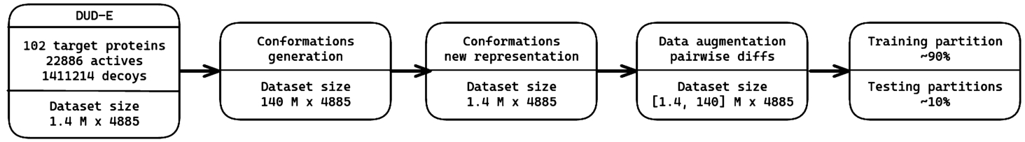
As for the molecular database used in this work, the Directory of Useful Decoys - Enhanced (DUD-E) (Mysinger et al., 2012) has been used to assess and validate the modelling proposal in this work. It is a target-ligand public database well-known in the field and is often used to validate and quantify the performance of a virtual screening methodology. Overall, it contains 102 target proteins and 22 886 active compounds: an average of 224 ligands per target. In addition, there are 50 decoys – or inactive compounds – for each active compound, having similar 1-D Physico-chemical properties to remove bias (e.g. molecular weight, calculated LogP) but different 2-D topology to be likely non-binders. The total number of compounds exceeds 1.4 million (22 886 actives, and 1 411 214 decoys).
Since the database contains rigid molecules, up to 100 3-D molecular conformations have been generated for every compound to consider its flexibility. Molecular descriptors are extracted from this extended database with conformations, generating new representations per pair of molecules. Then, for the main modelling proposal – gradient boosting – there is no more data preprocessing. For the rest of the comparative baselines, the preprocessing details are specified in Section 2.4.2.
Next, for the model training stage, the data is split into three parts: one for training that will be used with cross-validation using
This data preparation, specifically for the DUD-E dataset in these experiments, is the one generically described in Section 2.2. A visual representation showing how the dataset size evolves through this process can be seen in Fig. 2.
Fig. 2
From left to right, the dataset size evolution (number of samples x number of features) obtained through the data preparation pipeline. The number of samples obtained during the data augmentation (through pairwise differences) depends on whether the target proteins are exposed to the complete DUD-E or only their related ligands – 140 M in these experiments. Also note that not all target proteins have the same number of associated ligands (active or decoys).
More specifically, we have proceeded with the following data partitioning schema using all the 102 target proteins and their associated ligand compounds, either active or decoy. The same data partitioning schema, as well as random seeds, have been used for all the experiments run and baseline models:
• Data partition A: 96 out of the 102 target proteins along with their associated ligand compounds. The list of target proteins for this partition is: ACES, ADA, ADRB1, ADRB2, AKT2, ALDR, AMPC, AOFB, BACE1, BRAF, CAH2, CASP3, CDK2, COMT, CP2C9, CP3A4, CSF1R, CXCR4, DEF, DHI1, DPP4, DRD3, DYR, EGFR, ESR1, ESR2, FA10, FA7, FABP4, FAK1, FGFR1, FKB1A, FNTA, FPPS, GCR, GLCM, GRIA2, GRIK1, HDAC2, HDAC8, HIVINT, HIVPR, HIVRT, HMDH, HS90A, HXK4, IGF1R, INHA, ITAL, JAK2, KIF11, KIT, KITH, KPCB, LCK, LKHA4, MAPK2, MCR, MET, MK01, MK10, MK14, MMP13, MP2K1, NOS1, NRAM, PA2GA, PARP1, PDE5A, PGH1, PGH2, PLK1, PNPH, PPARA, PPARD, PPARG, PRGR, PTN1, PUR2, PYGM, PYRD, RENI, ROCK1, RXRA, SAHH, SRC, TGFR1, THB, THRB, TRY1, TRYB1, TYSY, UROK, VGFR2, WEE1, XIAP.
– Data partition A.1:
– Data partition A.2:
• Data partition B: 6 out of the 102 target proteins and their associated ligand compounds. The list of target proteins for this partition is: AKT1, ACE, AA2AR, ABL1, ANDR, ADA17. This selection has been made by hand to cope with one target compound per DUD-E subset: Diverse, Dud38, GPCR, Kinase, Nuclear, and Protease. This partition allows the assessment of the model with new targets and ligand compounds not seen before during training.
Finally, all the methods and experiments included in this work have been implemented in the distributed computer cluster managed by the Supercomputing and Algorithms research group at the University of Almeria (University of Almeria). More information about the cluster composition can be found in Supplementary Information 1.
3.2Hyperparameter Optimization
The training partition (A.1) has been used for the hyperparameter optimization (HPO) process for all the models (gradient boosting and the rest of the baselines) using 100 trials per HPO process. The HPO has been carried out using the state-of-the-art framework Optuna (Akiba et al., 2019). Details about the HPO search space and results are given for every model in Supplementary Information 2.
Gradient boosting. The search space has been defined as shown in Table 7, and the best found hyperparameter set is shown in Table 8.
Logistic regression. Table 9 shows the search space defined for the hyperparameter optimization process of the logistic regression model, and Table 10 shows the best-found hyperparameter set.
SVM – ensemble. Table 11 shows the search space for the hyperparameter optimization process of the SVM model, and Table 12 indicates the best-found hyperparameter set.
Random forests. Table 13 shows the search space for the hyperparameter optimization process of the random forest model, and Table 14 indicates the best-found hyperparameter set.
Deep neural network. Table 15 shows the search space for the hyperparameter optimization process of the deep learning model, Table 16 indicates the best-found hyperparameter set for the version with Z-score normalization, and Table 17, for the version without input data normalization.
3.3Activity Modelling Results
Results in terms of ROC-AUC are summarized in Table 3 for all the modelling approaches and data partitions. In addition, Figs. 3, 4, and 5 show the area under the ROC curve for the different data partitions (A.1, A.2, and B), respectively, and include all the modelling approaches.
Table 3
ROC AUC (Area under the receiver operating characteristic curve) for the different models and evaluated on the three data partitions.
| AUC | Data partition | ||
| Model | A.1 | A.2 | B |
| LR | 0.74073 | 0.73816 | 0.57002 |
| SVM-e | 0.83517 | 0.82335 | 0.70706 |
| RF | 0.99958 | 0.98542 | 0.78419 |
| DNN-Z | 0.98848 | 0.93944 | 0.65947 |
| DNN | 0.84338 | 0.82481 | 0.82999 |
| XGB | 0.99933 | 0.96384 | 0.87539 |
Algorithm name abbreviations: LR (logistic regression), SVM-e (support vector machines using an ensemble approach), RF (random forests), DNN-Z (deep neural network using Z-score normalization on input data), DNN (deep neural network without Z-score normalization), and XGB (gradient boosting using XGBoost).
Fig. 3
Receiver Operating Characteristic (ROC) showing the area under the curve (AUC) for every modelling approach when dealing with the training data partition (A.1). Algorithm name abbreviations: LR (logistic regression), SVM-e (support vector machines using an ensemble approach), RF (random forests), DNN-Z (deep neural network using Z-score normalization on input data), DNN (deep neural network without Z-score normalization), and XGB (gradient boosting using XGBoost).
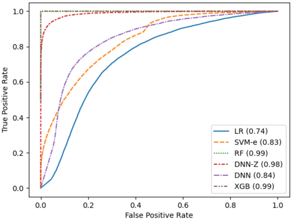
Fig. 4
Receiver Operating Characteristic (ROC) showing the area under the curve (AUC) for every modelling approach when dealing with the testing data partition (A.2). Algorithm name abbreviations: LR (logistic regression), SVM-e (support vector machines using an ensemble approach), RF (random forests), DNN-Z (deep neural network using Z-score normalization on input data), DNN (deep neural network without Z-score normalization), and XGB (gradient boosting using XGBoost).
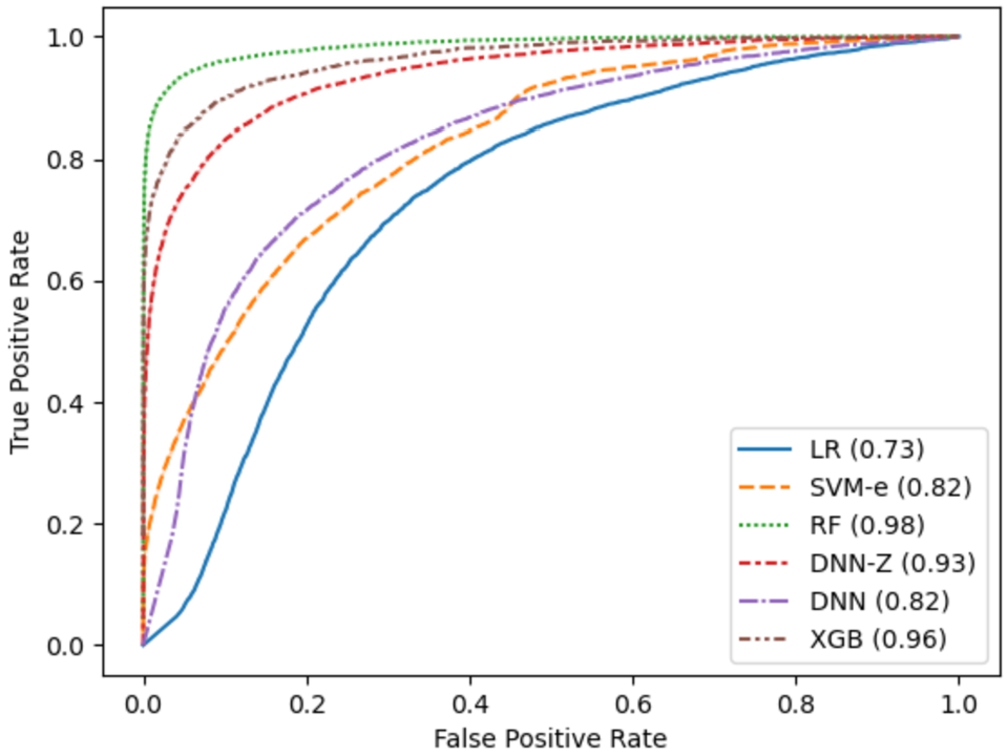
Fig. 5
Receiver Operating Characteristic (ROC) showing the area under the curve (AUC) for every modelling approach when dealing with the testing data partition (B). Algorithm name abbreviations: LR (logistic regression), SVM-e (support vector machines using an ensemble approach), RF (random forests), DNN-Z (deep neural network using Z-score normalization on input data), DNN (deep neural network without Z-score normalization), and XGB (gradient boosting using XGBoost).
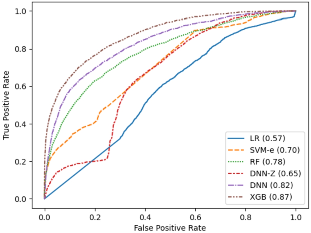
It can be seen that the gradient boosting (XGB) approach obtains a notable AUC performance in all three data partitions: 0.99 in A.1 (training), 0.96 in A.2 (testing with new ligands), and 0.87 in B (testing with new targets and new ligands). Even though the random forest (RF) model outperforms in the A.2 partition obtaining higher AUC (RF = 0.98 vs. XGB = 0.96), the RF AUC performance in the B partition is worse than XGB (RF = 0.78 vs. XGB = 0.87). We see this situation as most favourable to the XGB model as both obtain extremely high AUC values in the A.2 partition. However, the performance for XGB in the B partition is higher than RF. We consider the performance in this B partition extremely important as the models face both new target molecules and new ligand molecules not seen during training. This fact puts the RF model in a good position as an alternative, which could be expected as both modelling approaches share some algorithmic principles and how classification decision boundaries are shaped.
However, applying a basic approach, such as logistic regression (LR), results in much more modest AUC values. This result is not only due to the linearity constraint on the model decision boundary, where the AUC obtained in the B partition is still much worse than the AUC obtained either in A.1 or A.2. The reason behind this is probably the necessary data preprocessing applied in its training data and later being propagated to the prediction time for filling missing data gaps or data scaling.
The ensemble of support vector machines (SVM-e) obtains slightly better results than the LR model because SVM-e is able to shape classification decision boundaries with non-linearities. Even so, it suffers from the same problem as the LR approach, and the AUC performance on the B partition – with new targets and ligand compounds – is degraded, probably due to the required data preprocessing steps.
Finally, the deep neural network (DNN) model has been trained with two data preprocessing procedures: one (DNN) with just the basic steps, such as data imputation to fill gaps with missing data, and the other one (DNN-Z), including the data scaling using Z-normalization in addition. The goal is to evaluate the performance impact of data scaling, especially on the testing data partitions. Results show that DNN-Z obtains higher AUC on the training partition A.1 (DNN-Z = 0.98 vs. DNN = 0.84) and the testing partition A.2 with only new ligands (DNN-Z = 0.93 vs. DNN = 0.82). However, its performance worsens noticeably on the testing partition B with both new targets and ligands (DNN-Z = 0.65 vs. DNN = 0.82). The reason is probably the domain shift over the statistics used to scale the new unseen target and ligand compounds. An interesting fact is the performance stability over the three data partitions for the DNN approach, but below its competitors.
It can be concluded that the XGB approach provides the best performance in all the designed data partitions.
3.4Sensitivity Analysis for Molecular Conformations
As noted in Section 2.2, certain data preprocessing steps have been performed on the molecular descriptors, including reducing multiple conformations per molecule to a single conformational representative by taking the average of the multiple conformation values. Considering that the N conformations of a given molecule have been generated by rotating each torsion angle θ degrees in
Therefore, rather than viewing this as a potential weakness in information loss, this step is important and useful for adding robustness to estimation and optimization because it reduces the risk of frequency bias. However, it is important to validate this approach during the model inference using all the conformations in order to assess if there is a potential loss of quality in the response.
In this section, we use the XGB model trained for the experiments (Table 8), i.e. trained with the conformation reduction approach. Then, the model is used to perform the inference on the testing data partition B, but now without reducing the conformations to a single representative sample. Therefore, the samples in the dataset correspond to the Cartesian product of all the conformations between all the target proteins and all the ligand compounds. For a clearer understanding of how the dataset size changes, a visual representation is provided in Fig. 6. The goal of this experiment is to assess the sensitivity of the model to new conformations (molecular torsions) that were not directly observed during training due to changes in representation (refer to Fig. 2).
Fig. 6
From left to right, the dataset size evolution (number of samples x number of features) obtained through the data preparation pipeline. The number of samples obtained during the data augmentation (through pairwise differences) depends on whether the target proteins are exposed to the complete DUD-E or only their related ligands, 14000 M in this experiment.
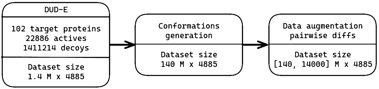
Fig. 7
Receiver Operating Characteristic (ROC) showing the area under the curve (AUC) for every modelling approach when dealing with the testing data partition (B). Comparison of test prediction data with the conformation transformation versus all the conformations, and using the same model built with XGB (gradient boosting using XGBoost) in both cases.
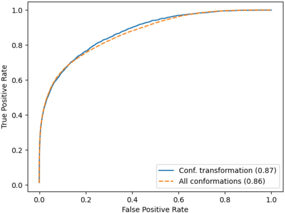
Figure 7 shows the ROC AUC results for the prediction over the same testing data partition B both by reducing the conformations and by performing the prediction for all combinations. It can be seen that both curves are almost identical (ROC AUC 0.87 vs. 0.86), so no performance loss is appreciated.
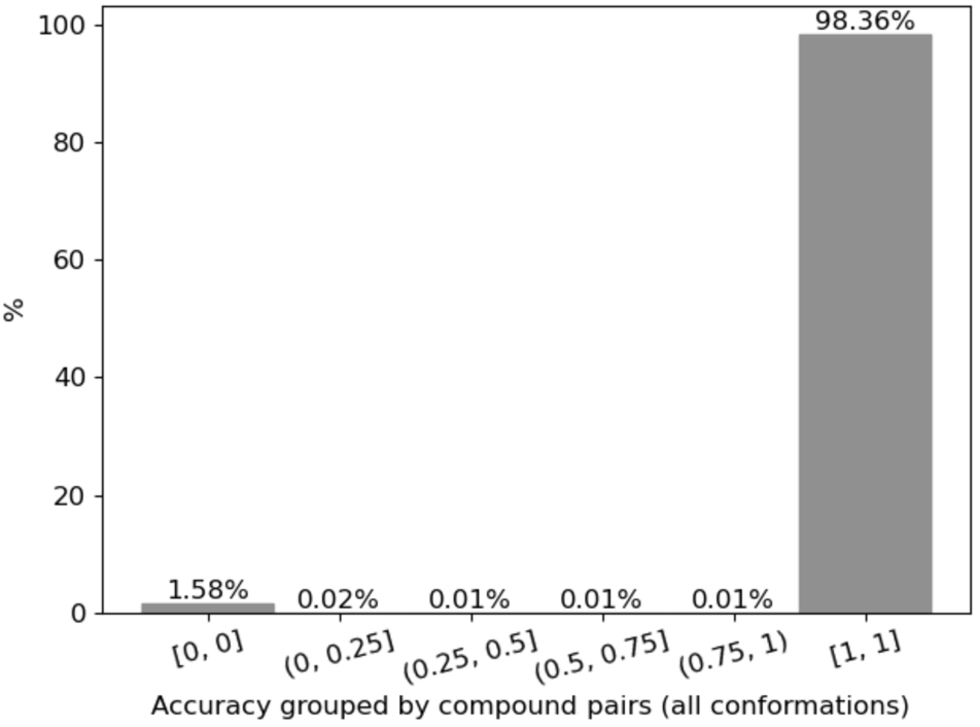
Another interesting analysis is checking the performance from a more detailed perspective by calculating the accuracy grouped by compound pairs from the testing data partition (B). Figure 8 indicates that
Indeed,
Fig. 8
Accuracy is grouped by compound pairs from the testing data partition (B). Each group corresponds to a pair
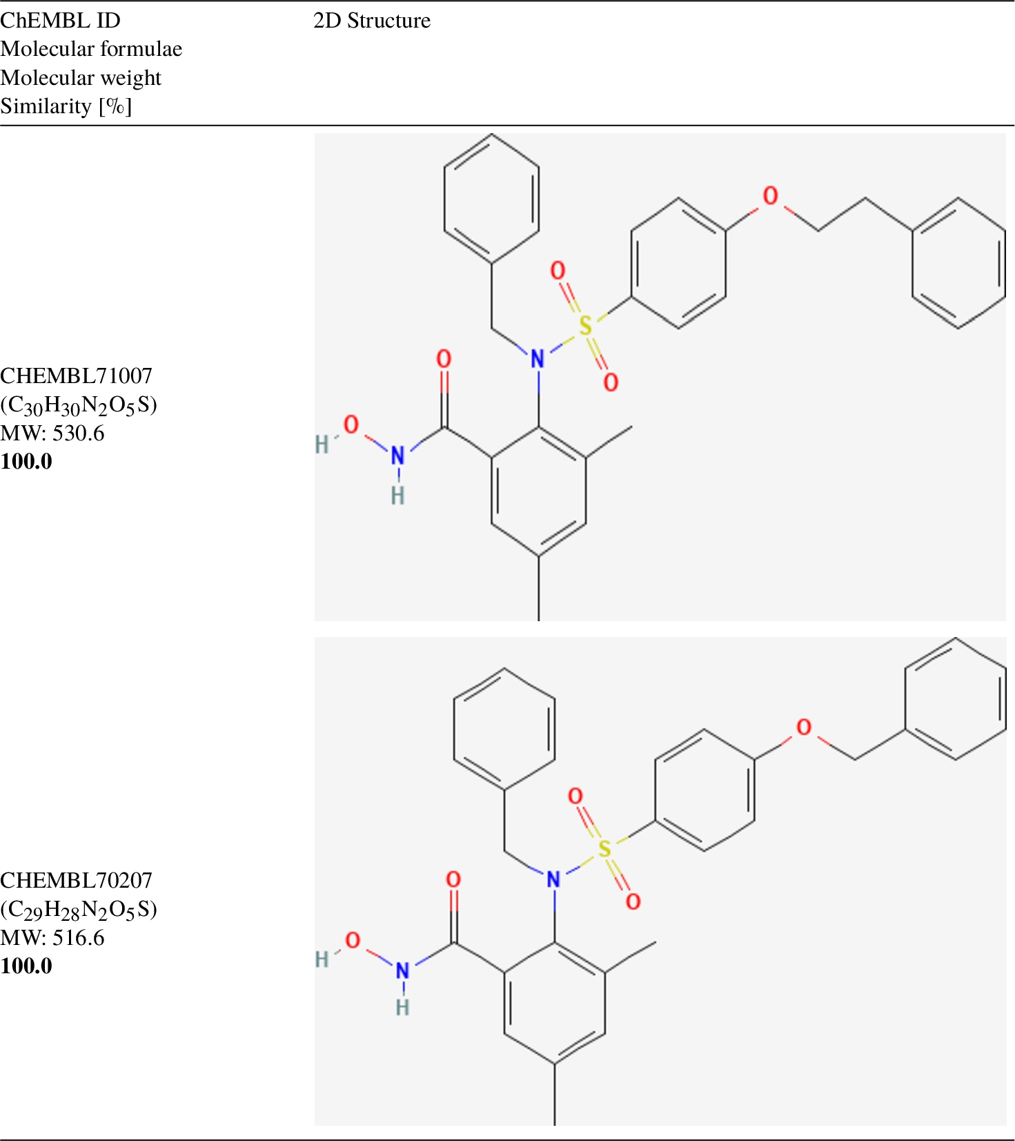
3.5Molecular Similarity Results
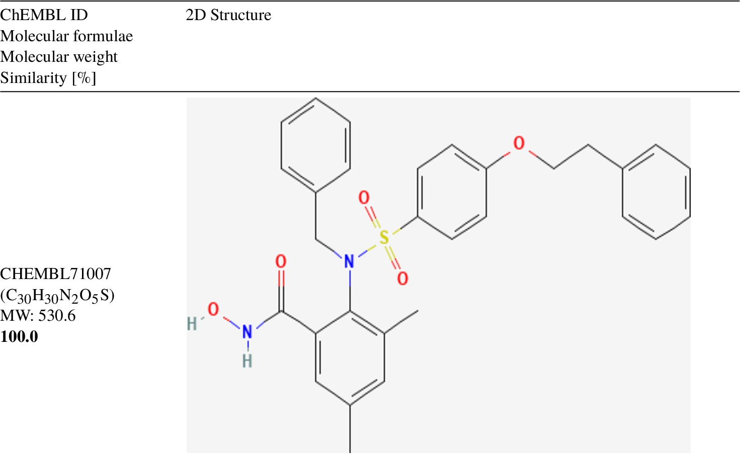
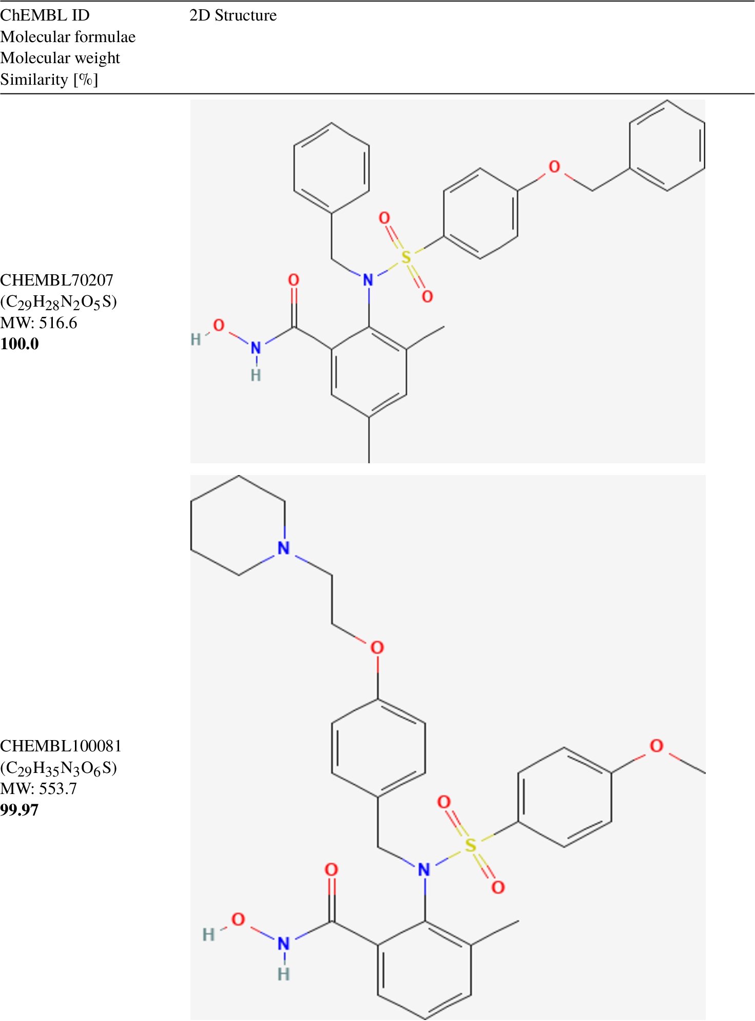
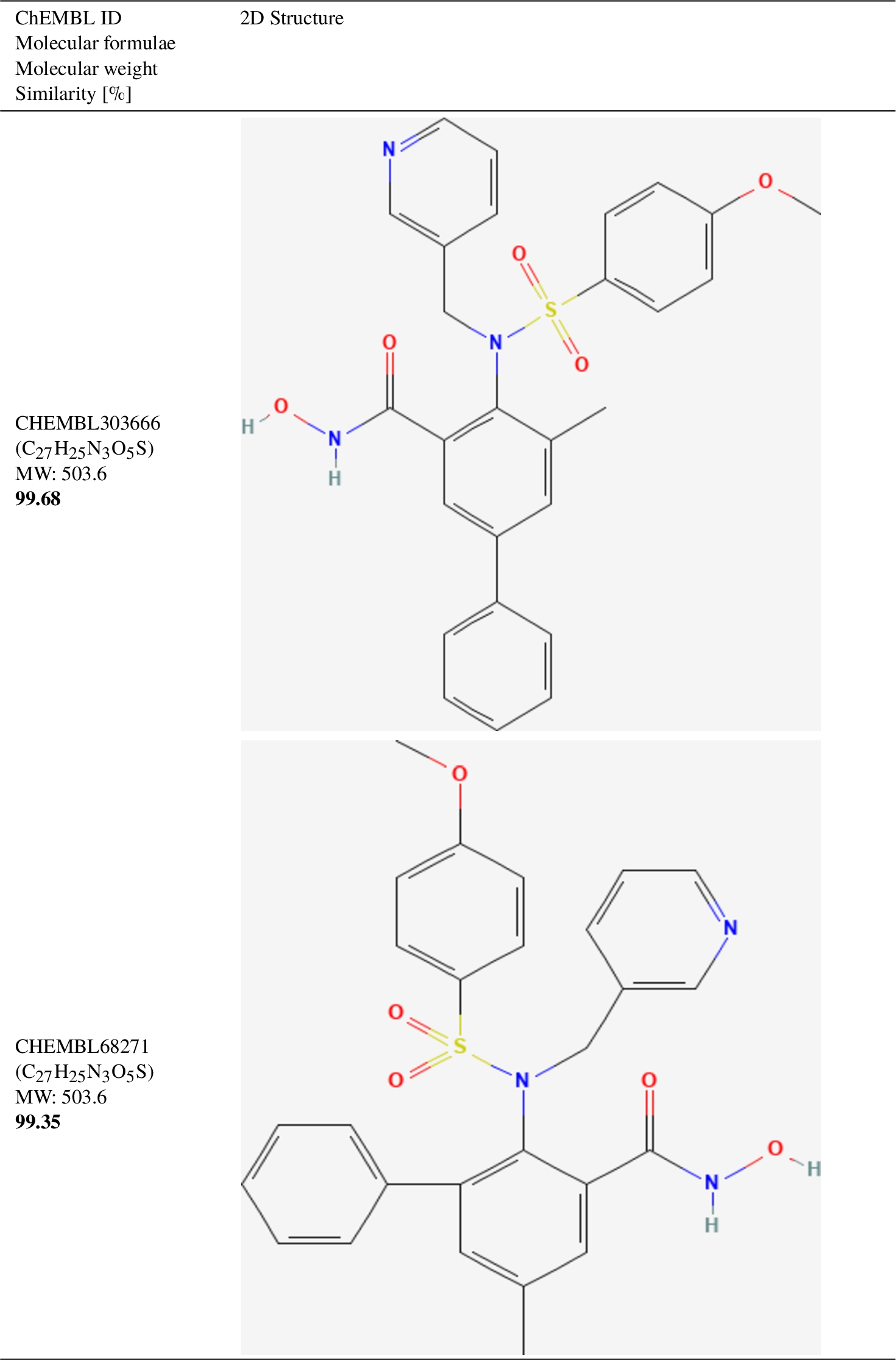
For testing the molecular similarity operation mode, two compounds have been selected from the testing data partition B (see Section 3.1). One is a small compound with ChEMBL ID CHEMBL190, and the other is a medium-sized compound with ChEMBL ID CHEMBL71007. However, all DUD-E database has been used as search space to find the top 5 most similar compounds.
As discussed in the introduction (Section 1), this is a subjective task, as there is no single way to determine the similarity between compounds. While some authors may consider the compounds’ shape to determine their similarity, others may consider other criteria.
For the similarity operation mode within the ALMERIA methodology presented in this work, two compounds (two ligands) are presented to the trained model that gives a response in
Despite the subjectivity, reasonable similarities between the first results can be appreciated. Results with the top-5 most similar compounds are shown in Table 18 for the small-sized compound, and Table 19 for the medium-sized compound. Furthermore, to validate our proposal, it is very important to remark that the first most similar compound is always the query compound with
Table 4
Top-1 similarity found in DUD-E for the small-sized compound CHEMBL190 (Molecular weight = 180.16).
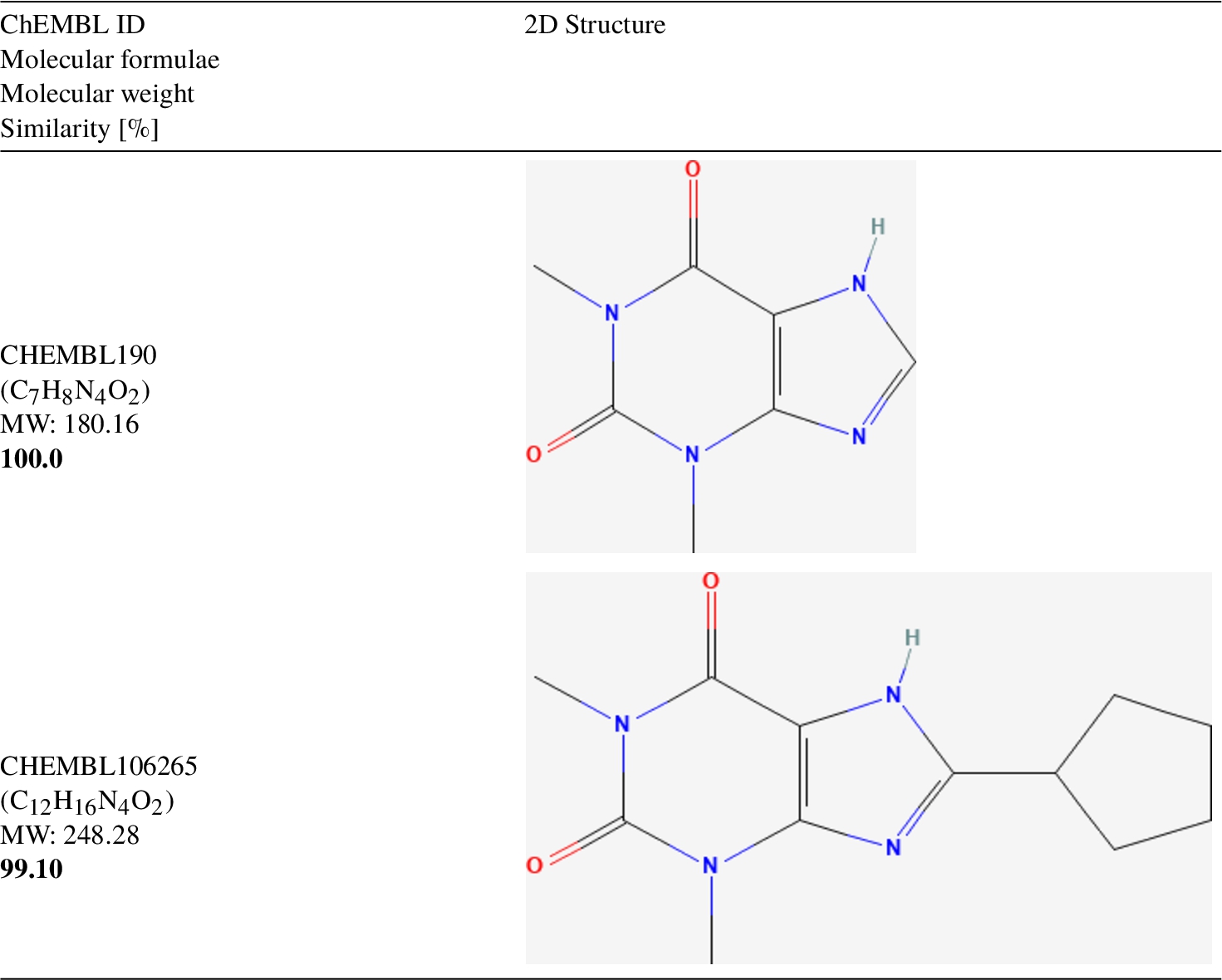
Table 5
Top-1 similarity found in DUD-E for the medium-sized compound CHEMBL71007 (Molecular weight = 530.6)
4Performance Measurement
In order to measure the performance in terms of computing times for the different steps in the process (see Fig. 1), only one node of the cluster has been used:
• For CPU computing mode: AMD EPYC Rome 7642 (48 cores) with 512 GB RAM and 240 GB SSD.
• For GPU computing mode: AMD EPYC Rome 7302 (16 cores) with 512 GB RAM and 240 GB SSD, 2x GPUs NVIDIA Tesla V100 with 32GB HBM2, 5120 CUDA cores, and 640 Tensor cores.
However, the shared network file system (NFS) has been used for disk input/output operations. It has significant repercussions on the first steps of the pipeline concerning the generation of conformations and descriptors.
A single protein target from the DUD-E database has been used to accelerate the performance measurements. The protein target is aa2ar, associated with
Table 6
Computing times for different pipeline steps. h, m, s stands for hours, minutes and seconds, respectively.
| Task | Time |
| Data preparation | |
| Generating maximum 100 conformations for each of the | 5 h 30 m |
| Generating molecular descriptors for each conformation from all the | 14 h |
| Data size for this single crystal aa2ar with maximum 100 conformations per compound: | |
| Reading database | 10 m |
| Reduce conformations to a single representative sample | < 2 m |
| Compound pair data transformation | < 1 m |
| Model building | |
| CV folds creation | < 1 m |
| Hyperparameter optimization with 100 trials and using 10-fold CV per trial (CPU) | 14 h |
| Hyperparameter optimization with 100 trials and using 10-fold CV per trial (GPU) | 6 h |
| Final model training | < 1 m |
| Model inference | |
| Activity and similarity prediction on full dataset with all compound pairs | < 1 s |
5Conclusion
A methodology (ALMERIA: Advanced Ligand Multiconformational Exploration with Robust Interpretable Artificial Intelligence) has been proposed to develop virtual screening software for estimating compound similarity and activity prediction. Its core is based on pairwise molecular contrasts while also considering the conformation variability. The great benefit is obtaining excellent classification rates on out-of-sample observations and having a quick response, even for a large batch of queries. Moreover, this proposal relies on artificial intelligence methods to exploit high-dimensional data instead of over-optimizing based on a specific criterion (e.g. shape).
As shown in Fig. 1 and described in Section 2, the ALMERIA methodology has covered the entire pipeline from data preparation to model selection and hyperparameter optimization. In this work, the implementation is based on scalable software and methods to exploit large volumes of data (in the order of several terabytes), and deployed in a distributed computer cluster using a real use case: the public access DUD-E database. However, the ALMERIA methodology is generic enough to be applied to any other database that exploits molecular contrasts.
The chosen data representation is based on numerical molecular descriptors, e.g. as generated by the Dragon software (Mauri et al., 2006), that are generated for each conformation of every molecule. These conformations were generated using OpenEye Scientific Omega software (Hawkins et al., 2010) with a limit of 100 conformations per molecule. Two transformations have been applied to these data representations:
1. Reducing multiple conformations for a given molecule to a single representative sample using the averaged descriptors values, thus reducing frequency bias on the model optimization process. Experiments and sensitivity analysis in Section 3.4 show that model response is consistent among multiple combinations of conformation pairs for different molecules.
2. Transforming the molecules’ descriptors to pairwise molecular contrasts using the absolute difference between their descriptor values. This has a data augmentation effect. This way, a single model may fit the entire database, therefore enjoying better generalization properties, as shown by the experiments in Section 3.3 on numerical molecular descriptors, like the one generated by the Dragon software (Mauri et al., 2006) for each conformation of every molecule. These conformations were generated using OpenEye Scientific Omega software (Hawkins et al., 2010) with a limit of 100 conformations per molecule.
A very important aspect of the ALMERIA methodology is the use of detailed data split criteria in addition to the cross-validation used during the HPO process. In this way, the models’ predictive performance is evaluated on different data partitions to assess their true generalization ability with protein targets and ligands not seen previously during training or validation. The designed data partitions for the use case in this work (DUD-E database) are shown in Section 3.1.
The underlying machine learning algorithm for similarity and activity prediction is based on a supervised classification model. Any model that satisfies these conditions may be plugged into the proposed pipeline (Fig. 1). Our main proposal is based on gradient boosting after studying the problem characteristics (Section 2.4.1), but other models, such as logistic regression, SVM ensemble, random forests, and deep neural net have been included to benchmark the performance. Every model architecture has been optimized using a thorough hyperparameter optimization process using 10-fold cross-validation.
The best molecular activity prediction results are obtained with the main modelling proposal gradient boosting, showing the state-of-the-art performance (ROC AUC: 0.99, 0.96, 0.87), especially with the data partition whose protein targets and ligands are new for the model. This result also proves that the chosen data representation and modelling have good generalizable properties.
As mentioned above, molecular conformation information is not neglected for every molecule but is used in a new data transformation instead. As this can be controversial, especially in the chemical field, a sensitivity analysis (Section 3.4) was performed, indicating that the model response is consistent and no performance loss is observed when the model is queried using a Cartesian product of all the molecular conformations.
Moreover, the modelling proposal has demonstrated that it may offer interesting and useful results for compound similarity (Section 3.5).
Finally, a small performance measurement exercise has been performed (Section 4) to measure the elapsed time (in CPU or GPU computing mode) for every important step within the ALMERIA methodology pipeline. The model efficiency allows us to respond quickly, even for a large batch of queries.
In future work, we will consider the use of additional molecular databases both for performing the inference with the model trained here and applying the entire methodology with additional merged databases. Moreover, it would be interesting to perform a more in depth interpretability analysis, even accommodating causality tools and collaboration with additional experts in the field of chemistry.
Although a probability value
Future efforts will be put on letting the system be able to perform online learning, i.e. to update the already learned model with new data as it is collected. This should not be a great challenge as the specific gradient boosting implementation (XGBoost) already allows to perform incremental updates.
We are also working on an online front end service as interface for the back end methodology that we show in this work.
Lastly, we have identified several potential applications and end-users who could greatly benefit from the ALMERIA development:
• Applications:
– Virtual screening: ALMERIA helps narrow down vast databases of potential drug candidates by predicting their activity and similarity to known drugs. This saves time and money in the early stages of drug development.
– Identifying new leads: By analysing large datasets, ALMERIA can identify promising new molecules with potential drug-like properties that might not have been considered before.
• End users:
– Pharmaceutical companies: These companies are constantly searching for new drugs. ALMERIA can significantly accelerate their drug discovery pipelines.
– Biotech startups: Smaller companies often lack the resources for large-scale drug discovery efforts. ALMERIA’s efficiency and scalability can be a valuable asset for them.
– Academic researchers: Researchers can use ALMERIA to explore potential drug candidates for specific diseases or biological targets.
The data used in this work is the “Database of Useful Decoys Enhanced” (DUD-E) and it is publicly available in its web page: https://dude.docking.org/.
Notes
1 Even though any distance metric could be used, in practice, those that are naturally bounded, such as Jaccard/Tanimoto or cosine similarity, are more typically used given their better interpretability.
Appendices
Supplementary Information 1
Supplementary Information 1Cluster composition
Briefly, the cluster has a total of 33 nodes with 74 CPUs + 15 GPUs (1 380 cores, 9 TB of RAM, and 25 TB of solid-state storage) that are distributed over an Infiniband network as follows:
• Front-end: Bullx R423E3i. 2 Intel Xeon E5 2620 2 GHz (12 cores) and 64 GB RAM. RAID disk with 16 TB.
• 8x Bull Sequana X440-A5: 2 AMD EPYC Rome 7642 (48 cores) and 512 GB RAM. 240 GB SSD.
• 2x Bull Sequana X410-A5: 2 AMD EPYC Rome 7302 (16 cores) and 512 GB RAM. 240 GB SSD.
– 4x GPUs NVIDIA Tesla V100 with 32GB HBM2, 5 120 CUDA cores and 640 Tensor cores.
• 2x Bullx R421-E4: 2 Intel Xeon E5 2620v3 (12 cores) and 64 GB RAM. 1 TB HDD.
– 2x NVIDIA K80: 2 Kepler GK210 with 24 GB GDDR5 and 4 992 cores CUDA.
– AMD ATI SAPPHIRE FIRE PRO S9100: 2 560 stream processors and 12 GB GDDR5.
• Bullion S8: 8 Intel Xeon E7 8860v3 (16 cores) and 2.3 TB RAM. 2x 300 GB SAS.
• 18x Bullx R424-E3: 2 Intel Xeon E5 2650 (16 cores) and 64 GB RAM. 128 GB SSD.
• 2x Bullx R424-E3: 2 Intel Xeon E5 2650v2 (16 cores) and 128 GB RAM. 1 TB HDD.
• 2x NextIO 2070.
– 4x GPUs Tesla M2070 (1792 cores).
Supplementary Information 2
Supplementary Information 2Hyperparameter optimization design and results
Table 7
Search space used during the hyperparameter optimization (HPO) process for fine-tuning the XGBoost model.
| Hyperparameter | Search space | Description |
| Grow policy | Split either at nodes closest to the root or at nodes with highest loss change. | |
| No. of estimators | Number of boosting iterations. | |
| Learning rate | Step size shrinkage used in update to prevent overfitting. | |
| Maximum depth | Maximum depth per boosting iteration (tree). | |
| Min. child weight | Minimum sum of instance weight (Hessian) needed in a child. | |
| Alpha | L1 regularization term on weights. | |
| Lambda | L2 regularization term on weights. | |
| Min. split loss | Minimum loss reduction required to make a further partition on a leaf node of the tree. | |
| Max. delta step | Values higher than zero make the update step more conservative. | |
| Subsample | Subsample ratio of the training instances in every boosting iteration. | |
| Columns subsample | Subsample ratio of columns in every boosting iteration. |
Table 8
Best hyperparameter set found after the HPO process for the XGBoost model.
| Hyperparameter | Value |
| Grow policy | ‘lossguide’ |
| No. of estimators | 992 |
| Learning rate | 0.05 |
| Maximum depth | 9 |
| Min. child weight | 5 |
| Alpha | 0.5 |
| Hyperparameter | Value |
| Lambda | 2.0 |
| Min. split loss | 0.5 |
| Max. delta step | 5.0 |
| Subsample | 1.0 |
| Columns subsample | 0.4 |
Table 9
Search space used during the hyperparameter optimization (HPO) process for fine-tuning the logistic regression model.
| Hyperparameter | Search space | Description |
| Penalty | Norm of the penalty for the bias/variance trade-off. | |
| C | Inverse of regularization strength; smaller values specify stronger regularization. |
Table 10
Best hyperparameter set found after the HPO process for the logistic regression model.
| Hyperparameter | Value |
| Penalty | |
| C | 0.001 |
Table 11
Search space used during the hyperparameter optimization (HPO) process for fine-tuning the SVM model.
| Hyperparameter | Search space | Description |
| Kernel | Kernel type for every SVM instance. | |
| C | Inverse of regularization strength; smaller values specify stronger |
Table 12
Best hyperparameter set found after the HPO process for the SVM model.
| Hyperparameter | Value |
| Kernel | |
| C | 0.5 |
Table 13
Search space used during the hyperparameter optimization (HPO) process for fine-tuning the random forest model.
| Hyperparameter | Search space | Description |
| Split criterion | The function to measure the quality of a split. | |
| No. of estimators (trees) | The number of trees in the forest. | |
| Min. samples split | The minimum number of samples required to split an internal node. |
Table 14
Best hyperparameter set found after the HPO process for the random forest model.
| Hyperparameter | Value |
| Split criterion | |
| No. of estimators (trees) | 10000 |
| Min. samples split | 4 |
Table 15
Search space used during the hyperparameter optimization (HPO) process for fine-tuning the deep learning model.
| Hyperparameter | Search space | Description |
| Batch size | Batch size for every gradient update. | |
| Optimization algorithm | – | |
| Initial learning rate | Initial learning rate used by the optimization algorithm. | |
| Learning rate scheduler | – | |
| Activation function | Activation function for the neurons in Dense layers. | |
| Dropout rate | Dropout rate. | |
| N | Number of feed-forwarded sub-blocks for the first part. | |
| M | Number of feed-forwarded sub-blocks for the second part. |
Table 16
Best hyperparameter set found after the HPO process for the final deep learning model with a total of 66.7 million trainable parameters. Version that normalizes input data with Z-score.
| Hyperparameter | Value |
| Batch size | 512 |
| Optimization algorithm | Adam |
| Initial learning rate | |
| Learning rate scheduler | |
| Activation function | relu |
| Dropout rate | 0.5 |
| N | 4 |
| M | 0 |
Table 17
Best hyperparameter set found after the HPO process for the final deep learning model with a total of 66.7 million trainable parameters. Version that does not normalize input data.
| Hyperparameter | Value |
| Batch size | 1024 |
| Optimization algorithm | Adam |
| Initial learning rate | |
| Learning rate scheduler |
| Hyperparameter | Value |
| Activation function | selu |
| Dropout rate | 0.7 |
| N | 0 |
| M | 4 |
Supplementary Information 3
Supplementary Information 3Molecular Similarity Results
Table 18
Top-5 similarity found in DUD-E for the small-sized compound CHEMBL190 (Molecular weight = 180.16).
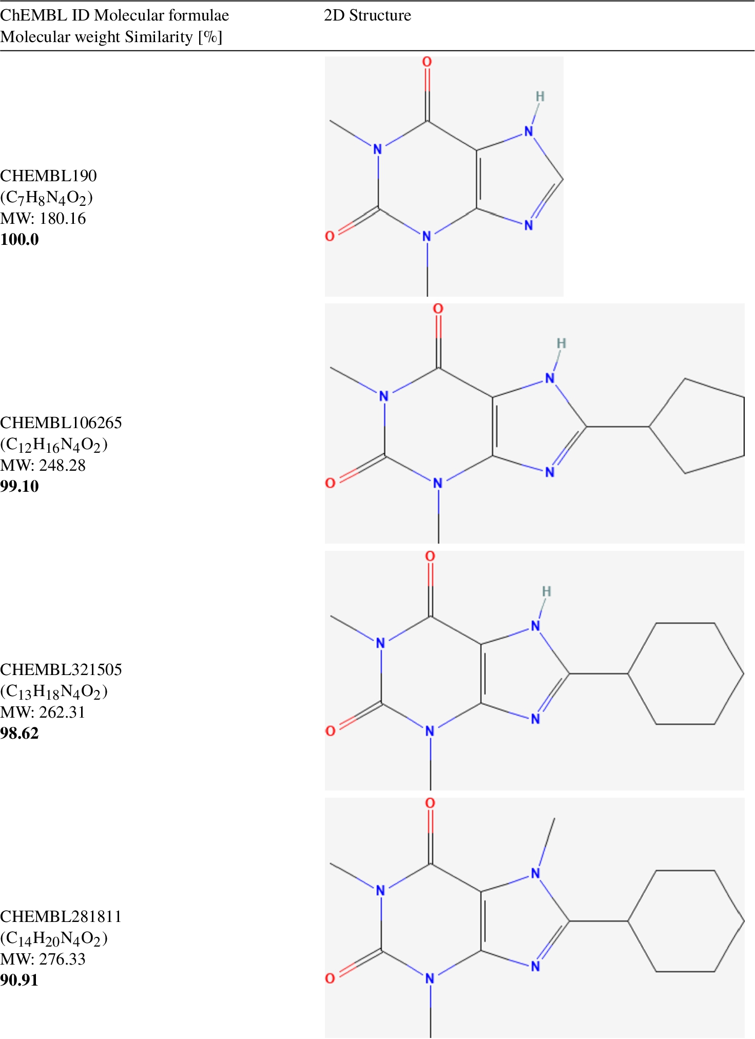
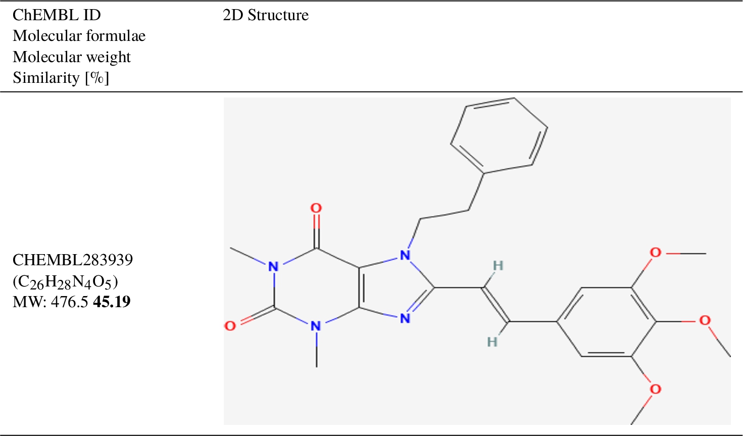
Table 19
Top-5 similarity found in DUD-E for the medium-sized compound CHEMBL71007 (Molecular weight = 530.6).
References
1 | Akiba, T., Sano, S., Yanase, T., Ohta, T., Koyama, M. ((2019) ). Optuna: a next-generation hyperparameter optimization framework. In: Proceedings of the 25rd ACM SIGKDD International Conference on Knowledge Discovery and Data Mining, 2623–2631. https://doi.org/10.1145/3292500.3330701. |
2 | Banegas-Luna, A.-J., Cerón-Carrasco, J.P., Pérez-Sánchez, H. ((2018) ). A review of ligand-based virtual screening web tools and screening algorithms in large molecular databases in the age of big data. Future Medicinal Chemistry, 10: (22), 2641–2658. https://doi.org/10.4155/fmc-2018-0076. |
3 | Bishop, C.M. ((2006) ). Pattern Recognition and Machine Learning. Information Science and Statistics. Springer, New York. 978-0-387-31073-2. |
4 | Breiman, L. (1997). Arcing the Edge. Technical Report 486, Statistics Department, University of California at Berkeley. |
5 | Breiman, L. ((2001) ). Random forests. Machine Learning, 45: (1), 5–32. https://doi.org/10.1023/A:1010933404324. |
6 | Breiman, L., Friedman, J.H., Olshen, R.A., Stone, C.J. ((1984) ). Classification and Regression Trees. Wadsworth. 0-534-98053-8. |
7 | Cereto-Massagué, A., Ojeda, M.J., Valls, C., Mulero, M., Garcia-Vallvé, S., Pujadas, G. ((2015) ). Molecular fingerprint similarity search in virtual screening. Methods, 71: , 58–63. https://doi.org/10.1016/j.ymeth.2014.08.005. https://www.sciencedirect.com/science/article/pii/S1046202314002631. |
8 | Chen, T., Guestrin, C. ((2016) ). XGBoost: a scalable tree boosting system. In: Proceedings of the 22nd ACM SIGKDD International Conference on Knowledge Discovery and Data Mining, KDD ’16, San Francisco, California, USA. Association for Computing Machinery, New York, NY, USA, pp. 785–794. 978-1-4503-4232-2. https://doi.org/10.1145/2939672.2939785. |
9 | Cheng, Z., Yan, C., Wu, F., Wang, J. ((2021) ). Drug-target interaction prediction using multi-head self-attention and graph attention network. IEEE/ACM Transactions on Computational Biology and Bioinformatics, 19: (4), 2208–2218. https://doi.org/10.1109/TCBB.2021.3077905. |
10 | Cherkasov, A., Muratov, E.N., Fourches, D., Varnek, A., Baskin, I.I., Cronin, M., Dearden, J., Gramatica, P., Martin, Y.C., Todeschini, R., Consonni, V., Kuz’min, V.E., Cramer, R., Benigni, R., Yang, C., Rathman, J., Terfloth, L., Gasteiger, J., Richard, A., Tropsha, A. ((2014) ). QSAR modeling: where have you been? Where are you going to? Journal of Medicinal Chemistry, 57: (12), 4977–5010. https://doi.org/10.1021/jm4004285. |
11 | Dask Development Team (2016). Dask: Library for dynamic task scheduling. https://dask.org. |
12 | Deng, J., Yang, Z., Ojima, I., Samaras, D., Wang, F. ((2021) ). Artificial intelligence in drug discovery: applications and techniques. Briefings in Bioinformatics, 23: (1). https://doi.org/10.1093/bib/bbab430. |
13 | Friedman, J.H. ((2001) ). Greedy function approximation: a gradient boosting machine. The Annals of Statistics, 29: (5), 1189–1232. https://doi.org/10.1214/aos/1013203451. |
14 | Furui, K., Ohue, M. (2022). Compound virtual screening by learning-to-rank with gradient boosting decision tree and enrichment-based cumulative gain. arXiv:2205.02169. https://doi.org/10.48550/ARXIV.2205.02169. |
15 | Hawkins, P.C.D., Skillman, A.G., Warren, G.L., Ellingson, B.A., Stahl, M.T. ((2010) ). Conformer Generation with OMEGA: algorithm and validation using high quality structures from the protein databank and Cambridge structural database. Journal of Chemical Information and Modeling, 50: (4), 572–584. https://doi.org/10.1021/ci100031x. |
16 | Hu, H., Bajorath, J. ((2020) ). Activity cliffs produced by single-atom modification of active compounds: systematic identification and rationalization based on X-ray structures. European Journal of Medicinal Chemistry, 207: , 112846. https://doi.org/10.1016/j.ejmech.2020.112846. https://www.sciencedirect.com/science/article/pii/S0223523420308187. |
17 | Huang, X., Khetan, A., Cvitkovic, M., Karnin, Z. (2020). TabTransformer: Tabular Data Modeling Using Contextual Embeddings. arXiv:2012.06678. https://doi.org/10.48550/ARXIV.2012.06678. |
18 | Hung, C., Gini, G. ((2021) ). QSAR modeling without descriptors using graph convolutional neural networks: the case of mutagenicity prediction. Molecular Diversity, 25: (3), 1283–1299. https://doi.org/10.1007/s11030-021-10250-2. |
19 | Jiang, Z., Xu, J., Yan, A., Wang, L. ((2021) ). A comprehensive comparative assessment of 3D molecular similarity tools in ligand-based virtual screening. Briefings in Bioinformatics, 22: (6), 231. https://doi.org/10.1093/bib/bbab231. |
20 | Jiménez, J., Škalič, M., Martínez-Rosell, G., De Fabritiis, G. ((2018) ). KDEEP: protein–ligand absolute binding affinity prediction via 3D-convolutional neural networks. Journal of Chemical Information and Modeling, 58: (2), 287–296. https://doi.org/10.1021/acs.jcim.7b00650. |
21 | Kimber, T.B., Chen, Y., Volkamer, A. ((2021) ). Deep learning in virtual screening: recent applications and developments. International Journal of Molecular Sciences, 22: (9). https://doi.org/10.3390/ijms22094435. |
22 | Kumar, A., Zhang, K.Y.J. (2018). Advances in the development of shape similarity methods and their application in drug discovery. Frontiers in Chemistry, 6. https://www.frontiersin.org/article/10.3389/fchem.2018.00315. |
23 | Li, J., Jiang, X. ((2021) ). Mol-BERT: an effective molecular representation with BERT for molecular property prediction. Wireless Communications and Mobile Computing, 2021: , 7181815. https://doi.org/10.1155/2021/7181815. |
24 | Maggiora, G., Vogt, M., Stumpfe, D., Bajorath, J. ((2014) ). Molecular similarity in medicinal chemistry. Journal of Medicinal Chemistry, 57: (8), 3186–3204. https://doi.org/10.1021/jm401411z. |
25 | Mao, J., Akhtar, J., Zhang, X., Sun, L., Guan, S., Li, X., Chen, G., Liu, J., Jeon, H.-N., Kim, M.S., No, K.T., Wang, G. ((2021) ). Comprehensive strategies of machine-learning-based quantitative structure-activity relationship models. iScience, 24: (9), 103052. https://doi.org/10.1016/j.isci.2021.103052. https://www.sciencedirect.com/science/article/pii/S2589004221010208. |
26 | Martin, Y.C., Kofron, J.L., Traphagen, L.M. ((2002) ). Do structurally similar molecules have similar biological activity? Journal of Medicinal Chemistry, 45: (19), 4350–4358. https://doi.org/10.1021/jm020155c. |
27 | Martínez, M.J., Razuc, M., Ponzoni, I. ((2019) ). MoDeSuS: a machine learning tool for selection of molecular descriptors in QSAR studies applied to molecular informatics. BioMed Research International, 2019: , 2905203. https://doi.org/10.1155/2019/2905203. |
28 | Mauri, A., Consonni, V., Pavan, M., Todeschini, R. ((2006) ). DRAGON software: an easy approach to molecular descriptor calculations. MATCH Communications in Mathematical and in Computer Chemistry, 56: (2), 237–248. |
29 | Mysinger, M.M., Carchia, M., Irwin, J.J., Shoichet, B.K. ((2012) ). Directory of useful decoys, enhanced (DUD-E): better ligands and decoys for better benchmarking. Journal of Medicinal Chemistry, 55: (14), 6582–6594. https://doi.org/10.1021/jm300687e. |
30 | Plewczynski, D., Łaźniewski, M., Augustyniak, R., Ginalski, K. ((2011) ). Can we trust docking results? Evaluation of seven commonly used programs on PDBbind database. Journal of Computational Chemistry, 32: (4), 742–755. https://doi.org/10.1002/jcc.21643. |
31 | Puertas-Martín, S., Redondo, J.L., Ortigosa, P.M., Pérez-Sánchez, H. ((2019) ). OptiPharm: an evolutionary algorithm to compare shape similarity. Scientific Reports, 9: (1), 1398. https://doi.org/10.1038/s41598-018-37908-6. |
32 | Ruiz Puentes, P., Valderrama, N., González, C., Daza, L., Muñoz-Camargo, C., Cruz, J.C., Arbeláez, P. ((2021) ). PharmaNet: pharmaceutical discovery with deep recurrent neural networks. PLOS ONE, 16: (4), 0241728. https://doi.org/10.1371/journal.pone.0241728. |
33 | Samanta, S., O’Hagan, S., Swainston, N., Roberts, T.J., Kell, D.B. ((2020) ). VAE-Sim: a novel molecular similarity measure based on a variational autoencoder. Molecules (Basel, Switzerland), 25: (15), 3446. https://doi.org/10.3390/molecules25153446. |
34 | Shahlaei, M. ((2013) ). Descriptor selection methods in quantitative structure-activity relationship studies: a review study. Chemical Reviews, 113: (10), 8093–8103. https://doi.org/10.1021/cr3004339. |
35 | Shen, C., Hu, Y., Wang, Z., Zhang, X., Pang, J., Wang, G., Zhong, H., Xu, L., Cao, D., Hou, T. ((2021) ). Beware of the generic machine learning-based scoring functions in structure-based virtual screening. Briefings in Bioinformatics, 22: (3), 070. https://doi.org/10.1093/bib/bbaa070. |
36 | Stepniewska-Dziubinska, M.M., Zielenkiewicz, P., Siedlecki, P. ((2018) ). Development and evaluation of a deep learning model for protein–ligand binding affinity prediction. Bioinformatics, 34: (21), 3666–3674. https://doi.org/10.1093/bioinformatics/bty374. |
37 | University of Almeria Supercomputing and Algorithms (SAL) research group – HPC infrastructure. https://sites.google.com/ual.es/hpca/infrastructure/hpc-infrastructure. |
38 | Wallach, I., Heifets, A. ((2018) ). Most ligand-based classification benchmarks reward memorization rather than generalization. Journal of Chemical Information and Modeling, 58: (5), 916–932. https://doi.org/10.1021/acs.jcim.7b00403. |
39 | Wang, Y., Wang, J., Cao, Z., Barati Farimani, A. ((2022) ). Molecular contrastive learning of representations via graph neural networks. Nature Machine Intelligence, 4: (3), 279–287. https://doi.org/10.1038/s42256-022-00447-x. |
40 | Winter, R., Montanari, F., Noé, F., Clevert, D.-A. ((2019) ). Learning continuous and data-driven molecular descriptors by translating equivalent chemical representations. Chemical Science, 10: (6), 1692–1701. |
41 | Xu, Z., Wang, S., Zhu, F., Huang, J. ((2017) ). Seq2seq fingerprint: an unsupervised deep molecular embedding for drug discovery. In: Proceedings of the 8th ACM International Conference on Bioinformatics, Computational Biology, and Health Informatics, ACM-BCB ’17, Boston, Massachusetts, USA. Association for Computing Machinery, New York, NY, USA, pp. 285–294. 978-1-4503-4722-8. https://doi.org/10.1145/3107411.3107424. |
42 | Yin, Y., Hu, H., Yang, Z., Xu, H., Wu, J. ((2021) ). RealVS: toward enhancing the precision of top hits in ligand-based virtual screening of drug leads from large compound databases. Journal of Chemical Information and Modeling, 61: (10), 4924–4939. https://doi.org/10.1021/acs.jcim.1c01021. |
43 | GitHub – dmlc/xgboost: Scalable, Portable and Distributed Gradient Boosting Library (2024). https://github.com/dmlc/xgboost. |


