
Minimal Surfaces and the Plateau Problem: Numerical Methods and Applications
Abstract
This article offers a comprehensive overview of the results obtained through numerical methods in solving the minimal surface equation, along with exploring the applications of minimal surfaces in science, technology, and architecture. The content is enriched with practical examples highlighting the diverse applications of minimal surfaces.
1Introduction
Mathematics is an abstract science, but often abstract mathematical theories, equations and other objects can be given an attractive and easy-to-understand interpretation. One such example is minimal surfaces.
Surfaces of the least area called minimal surfaces, are encountered in many areas of science and engineering. In recent years, minimal surfaces have been intensively studied in the research of chemical microstructures and biomolecules. In architecture, minimal surfaces appear when designing the roofs of large buildings. In computer-aided design and image analysis, minimal surfaces are also studied. Soap films and other membranes passing through a fixed boundary provide mechanical examples of minimal surfaces. The interface between crystalline and organic matter in the hard shell of the sea urchins can be described as a minimal surface. The equation with prescribed mean curvature is closely related to the equation of minimal surfaces, which describes the capillary surface.
Many research articles deal with the applications of minimal surfaces (Ambrazevičius, 1981; Tråsdahl and Rønquist, 2011; Pan and Xu, 2011; Lipkovski and Lipkovski, 2015). The main object of this article is the boundary value problem of the minimal surface equation. The mathematical formulation of the problem is as follows: solution
(1)
(2)
This problem is named after Belgian physicist Joseph Plateau (1801–1883), who experimented with the minimal surfaces obtained by immersing a wire frame in soap solution.
This article provides an overview of the research results obtained by solving applied minimal surface problems in Lithuanian scientific institutions. These results are reviewed and interpreted in the general background of today’s approach. One of the authors’ goals is to supplement the theoretical results with illustrative material – graphs and photos of real-life minimal surface objects. This our article extends the results presented in conference proceedings (Sapagovas, 2023).
By the end of the 20th century, quite a lot of numerical methods of the Plateau problem had been created and analysed already, but only at the beginning of the 21st century, did the number of these methods start to multiply (Halbrecht, 2009; Pan and Xu, 2011; Tråsdahl and Rønquist, 2011; Čiupaila et al., 2013; Lipkovski and Lipkovski, 2015; Schumacher and Wardetzky, 2019; Sakakibara and Shimizu, 2022) because of obvious reason: the number of applications of the minimal surface equation for the various real-life mathematical modelling problems increased significantly at that time. This motivated us to present in this article both already known and successfully used numerical methods for finding minimal surfaces and examining new problems of minimal surface application.
The present paper is organised as follows. Section 2 presents some important historical aspects of the problem under consideration, which usually helps to understand the current issues of the day better. Section 3 reviews the numerical methods of solving the minimal surface equation, emphasizing their properties, advantages and disadvantages rather than the theoretical justification of these methods. The equation with the prescribed mean curvature is considered in Section 4, where we consider applied problems related to the calculation of the surface of a liquid drop. Perhaps to the greatest extent, Section 5 deals with classical and non-standard applied problems of minimal surfaces.
2Plateau Problem: Historical Review
The concept of the minimal surface originates with Joseph-Louis de Lagrange who in the 18th century considered the problem of finding the surface of minimal area, bounded by a given closed three-dimensional curve. He proved that if the surface equation can be represented in an explicit form
This definition of the minimal surface can be explained simplistically, i.e. if the surface is minimal, then at each point of it, one can draw two surface lines bending in opposite directions. Beware, this is not a definition, but a mere interpretation (Fig. 1, the saddle surface).
Fig. 1
Two examples of the minimal surfaces: saddle surface (left) and soap film stretched on the wireframe.
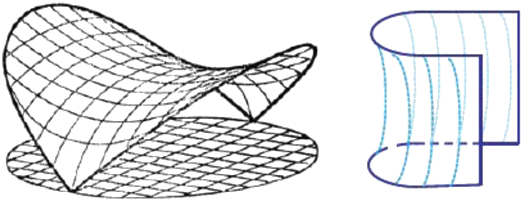
During the 18th and 19th centuries, many famous mathematicians were involved in developing the theory of minimal surfaces. Their effort led to the creation of a bundle of specific minimal surfaces, like catenoid or helicoid. For example, the catenoid (Fig. 2, on the right) arises as the catenary curve
Fig. 2
Catenary curve (left) and catenoid.

Fig. 3
Budapest at night. Bridge over the Danube River connecting Buda and Pest. The cables between the two main supports are in the shape close to the catenary. Photo: M. Sapagovas.
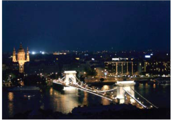
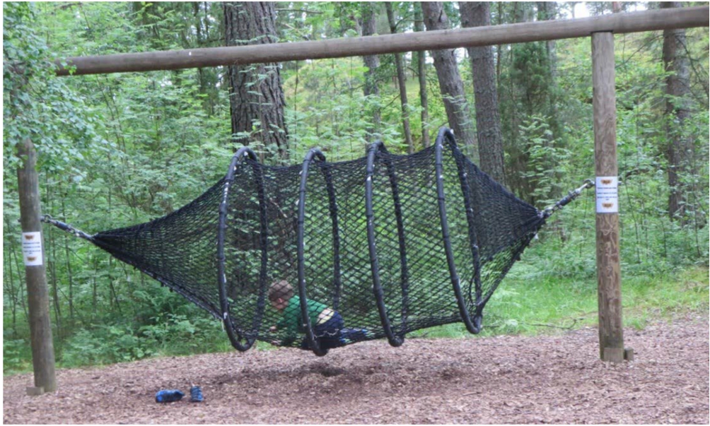
Fig. 5
The rope track in the Vaski Adventure Island (Photo from M. Sapagovas’s collections).
In 1849 Joseph Plateau demonstrated that the minimal surface can be obtained by immersing spatial wireframe into soap solution. He also noticed that the shape of such a surface is determined solely by the surface tension. Moreover, depending on the shape of the wireframe, several different minimal surfaces can be formed. In terms of differential equations, this means that depending on the boundary conditions subjected to the elliptical differential equation several different solutions (minimal surfaces) can be obtained. These Plateau’s experiments have drawn the attention of researchers in areas other than mathematics.
During the 18th and 19th centuries, there were several attempts to find the solution of the minimal surface equation corresponding to various shapes of the spatial boundary, including the presentation formulas for the solutions by Gaspard Monge (1776) and Karl Weierstrass (1866). However, they were generally regarded as practically unusable.
If there is not much success in finding the solution in an appropriate analytical form, then sooner or later the problem is subjected to the numerical methods of solution. In other words, the creation, and analysis of the numerical methods for the above mentioned problem come to the stage.
One of the founding works, where the numerical method of solution of the minimal surface equation was described is an article by Jesse Douglas, an American mathematician, published in Douglas (1927–1928). For his research in this field, Douglas was awarded the Fields Medal in 1936. After a few decades, the minimal surface equation was analysed by quite many researchers (Agalcev and Sapagovas, 1967; Concus, 1967; Greenspan, 1965; Johnson and Thomée, 1975), already.
It is worth mentioning, that the finite-difference method is the most popular method for differential problems. However, in the 1920s, when the general theory of the finite-difference methods was in its formation stage, the minimal surface equation was invincible for these methods. Therefore, the subsequent publications on the solution of the minimal surface equation appeared only three decades later, when this important problem was analysed independently by several researchers.
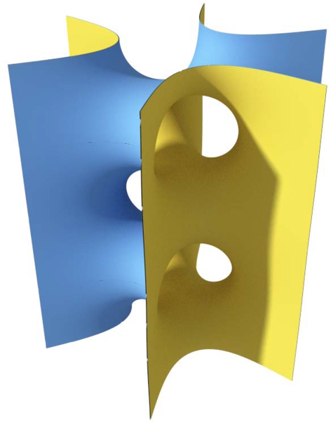
Fig. 7
A. Kasuba. Minimal Surfaces. Three Rings, 1986. Photo: A. Lukšėnas.
3Numerical Methods for the Plateau Problem
The main stages and a brief consideration of the characteristic features of the finite-difference method for the minimal surface equation will be presented here.
To begin with, we will assume that the domain of definition Ω of the problem (1)–(2) is a rectangle
Denote
1) a set of internal points
2) a set of boundary points
Let us substitute the differential problem (1)–(2) with the finite-difference problem at these points:
(3)
(4)
We will point out the main difficulties of solving the Plateau problem using the finite-difference method. Firstly, equation (3) at the point
Secondly, rearranging equation (1) into the form
It shows that in case
Thirdly, equation (1) represents only part of the variety of the minimal surfaces, those defined by the explicit equation
Those and many other obstacles foster the application of the numerical methods in the case of the Plateau problem. Various tools and techniques used by many researchers extend theoretical insights into the Plateau problem. Not a few researchers in the field of differential equations consider matter of honour to apply their method and solve the minimal surface equation.
4Equation with Prescribed Mean Curvature
Another equation, similar to the minimal surface equation is investigated intensively:
(5)
Capillarity refers to surface tension-driven phenomena appearing at fluid interfaces with a solid. Because of interaction forces, the surface of the fluid becomes distorted taking the shape of a concave or convex meniscus. Because of the surface tension, the liquid tends to take up a shape having minimal volume (minimal surface area, minimal free surface energy), showing the close relationship between capillarity and minimal surfaces. In mathematical terms, the two problems are related by the following common feature: both differential equations are nonlinear and non-uniformly elliptic with the coefficients depending on the gradient of the solution (Sapagovas, 1982, 1983; Vogel, 1987).
A. Ambrazevičius, while examining the boundary value problems of a certain class of nonlinear elliptic equations in conical domains, found the conditions for the existence and uniqueness of a sufficiently smooth classical solution of the capillarity problem (Ambrazevičius, 1981, 1991). Two features of this result can be pointed out. First, the result is proved in regions for which no assumption of invariability of the capillary cross-section is made. Second, this research includes the case where the shape of the surface of a liquid subjected to surface tension forces is sought under the additional condition that the volume of the liquid is given. Such fixed volume conditions of the fluid are characteristic of many modern problems of hydrostatics and hydrodynamics. It is also typical of the vibration technology problem discussed below.
The mean curvature equation (5) plays a significant role in various applications within vibration technology, as evidenced by its utilization in various items (Ragulskis et al., 1986). One notable example is its application in the design of liquid metal contacts (switches) controlled through magnetic interaction forces. Within the scope of the technological research project, the study of the mathematical model of liquid metal contact was initiated by Kaunas University of Technology professor K. Ragulskis (Zareckas and Ragulskienė, 1971; Ragulskis et al., 1986). Liquid metal contacts exhibit numerous advantageous properties, including high operational speed, exceptional reliability, resistance to vibration, and low, stable switching impedance. Additionally, they seamlessly integrate with various automation engineering components.
Fig. 8
Liquid metal contact.
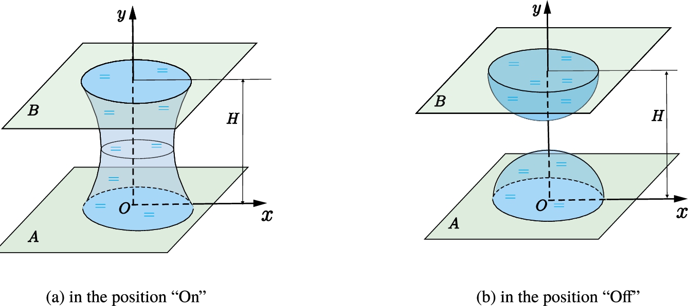
The design of such contacts adheres to specific technological requirements, notably the absence of a container, thereby enhancing operational reliability in any spatial orientation. In the case of liquid metals, such as mercury, the contact assumes the “On” position when a “bridge” connects two plates (Fig. 8a) and moves to the “Off” position when two drops of liquid adhere to distinct plates (Fig. 8b). In both scenarios, determining the free surface of the liquid drop involves solving a nonlinear differential problem. The associated differential equation is founded on the principle of minimum total energy, representing the sum of the liquid surface tension and gravitational potential energy.
For example, the free surface equation of a liquid drop of a given volume V is derived from the problem of minimisation of the sum of the gravitational energy
It is noteworthy that in the case the drop of an electroconductive liquid, such as mercury, is an electrical contact, the drop is adhered to the plane by special treatment (wetting), and the area of adhesion is a circle with radius R.
Fig. 9
Drop of liquid metal.
The Euler equation for the functional
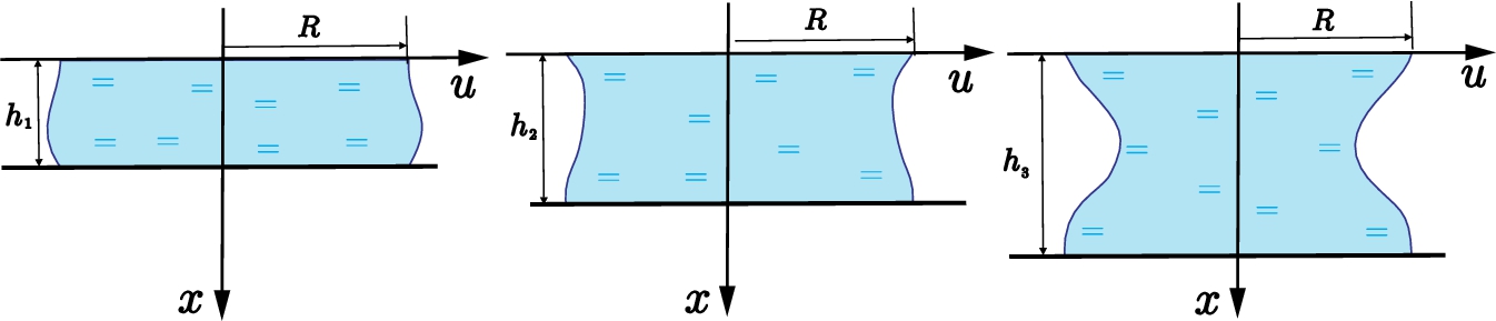
A mathematical model of a drop located between two parallel planes (Figs. 8, 10) is built analogously:
Fig. 10
Liquid metal contact between two plates in the position “On”. The influence of the distance between the planes on the shape of the drop.
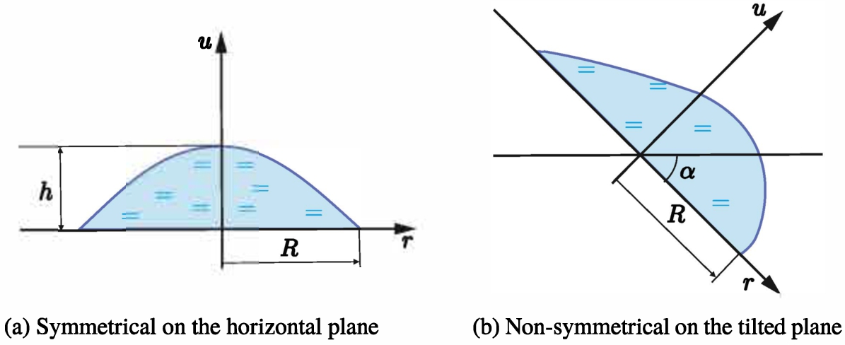
Under normal conditions, the shape of the free surface of the drop depends not much on the spatial position of the drop, which is an advantage of the electrical contacts of the liquid metal (Fig. 9a). However, in certain cases (e.g. in the presence of overloads, under the influence of inertial force, etc.), the effect of gravitational energy on the shape of the drop can be significant. In such cases, two-dimensional models of the free surface of the drop are used, including the model of the drop on an inclined plane (Fig. 9b) (Ragulskis et al., 1986):
Fig. 11
Irregular cases of liquid metal contact.
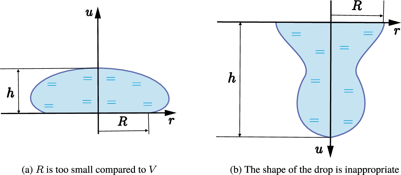
Numerical experiments were performed with all three mathematical models of the free surface of the drop indicated here, seeking to predict inappropriate drop shapes leading to unreliable operation of switches depending on the change of physical (
5Real-Life Applications of the Minimal Surfaces
During the 18th and 19th centuries, minimal surfaces were the object of investigation in various fields of mathematics, such as geometry, topology, theory of differential equations, control theory, mathematical physics, etc., or sometimes they were considered as a research method. In the second half of the 20th century, intensity of the application of minimal surfaces in physics, chemistry, biology, and technological problems grew significantly. Probably the fastest growth of the application of minimal surfaces was seen in certain areas of architecture and design, which is closely related to the trend of minimalism in visual arts.
Minimalism is an art movement that began in the 1960s and is characterized by rationality, simplified, and geometrized forms, seeking to disclose the structure of the subject. Minimalism also influenced the art of installations – spatial structures, designed for a specific place and time to create a unified experience and involving the audience.
The spread of minimal surfaces in architecture was fostered by a few factors. The first and the most obvious is that the surface of the least square requires the least amount of building materials. But this one is, probably, not the most important incentive. The next factor, which is much more important technologically is that due to the equal mean, curvature at any point of the surface mechanical tension is the same all over the surface, i.e. there are no critical points, where tension is higher compared to the other points of the surface. The third reason is hard to argue with: the shapes of minimal surfaces are very attractive.
The German architect Frei Otto was one of the first architects in the world to successfully apply minimal surface forms in architecture. The West German Pavilion created by him at the EXPO-67 exhibition in Montreal (Canada) became the first memorable example of a new architectural direction for many art fans. A few years later, a new architectural masterpiece by F. Otto appeared – the Munich Olympic Stadium (1972, Fig. 12). It should be noted that F. Otto was constantly interested in the design of lightweight structures and implemented his ideas at the Institute of Lightweight Structures and Conceptual Design in Stuttgart, which he founded himself.
Fig. 12
The roof tensile structures by Frei Otto of the Olympiapark, Munich, 1972. Foto: Dave Morris from Edinburgh, UK.
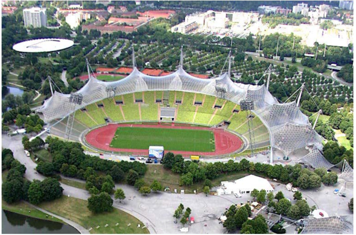
Fig. 13
Six-leaf clover-shaped minimal surface building in Valencia “Valencia L’Oceanografic”, the underwater restaurant. Architect F. Candela. Photo: F. Gabaldón, 2010.
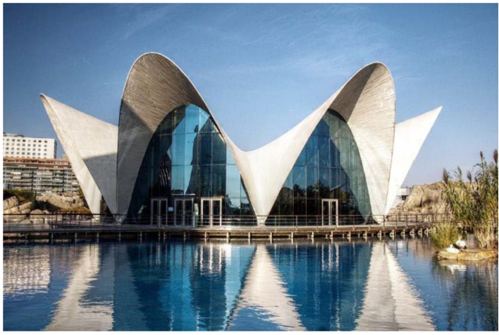
Fig. 14
Loro Park on the island of Tenerife, 2008. From M. Sapagovas’s photo collections.
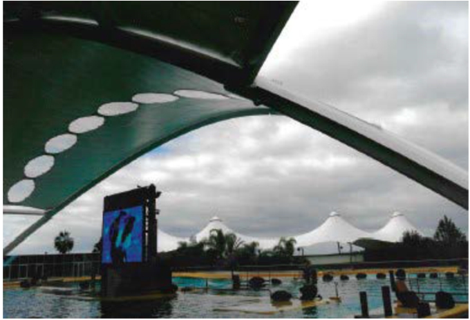
Fig. 15
Swarovski crystal museum at Innsbruck, 1998. Photo: M. Sapagovas.
Speaking about F. Otto’s work, let’s briefly return to the direction of architectural minimalism. After minimalism freed itself from strict geometric frameworks and moved to modern technologies, the perception of form changed, and the further development of minimalism was influenced by the possibilities provided by conceptual virtual modelling. Obeying these trends, F. Otto began to use not only J. Plateau’s modelling method (immersion of a wireframe in soap solution) to create new forms but also another modern possibility – solving the minimal surface equation by computer. These are the circumstances of the birth of new architectural masterpieces. F. Otto’s architectural ideas are described in Drew (1976), Otto and Rasch (1996), Lipkovski and Lipkovski (2015) and other books.
The Spanish Mexican architect Félix Candela designed several dozen restaurants and other buildings (mostly in Mexico and Spain) with minimal surface roofs resembling a six-leaf clover (Fig. 13). Today, in many European countries, there are quite a lot of stationary architectural objects with light minimal surface roofs. These are airport buildings, museums, and sports halls (Fig. 15). There are also temporary pavilions for various events, outdoor cafes, and concerts, as well as permanent industrial buildings (Figs. 16–18). In the Canary Islands, the minimal surfaces blend nicely with the dolphinarium pools (Fig. 14).
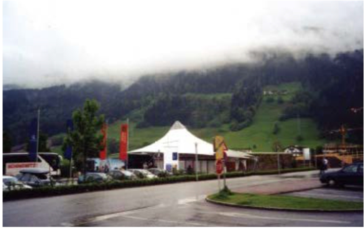
Fig. 16
Campaign to support the disabled. Vienna, city centre, 1998. Photo: M. Sapagovas.
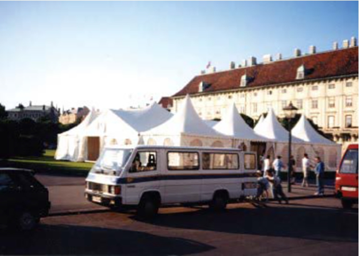
Fig. 17
Stockholm. Fair near the Royal Palace, 2021. From M. Sapagovas’s photo collections.
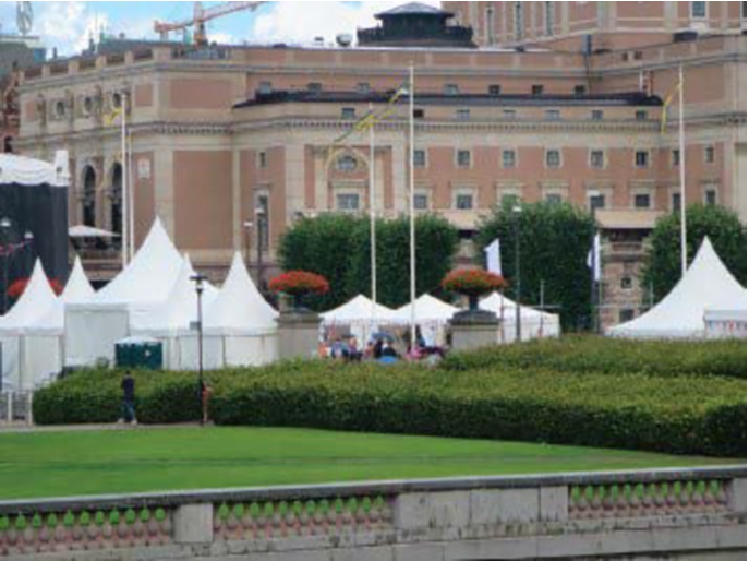
Fig. 18
Ventilation cooling towers (forced draft) and natural draft cooling tower located at power station Westfalen. Replacing part of the cylindrical surface with a minimal one increases the wind resistance of the tower.
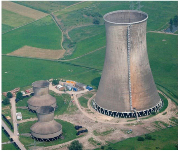
Fig. 19
Vilniaus Vingis Park stage is a classic example of minimal surfaces in architecture. Photo: M. Sapagovas.
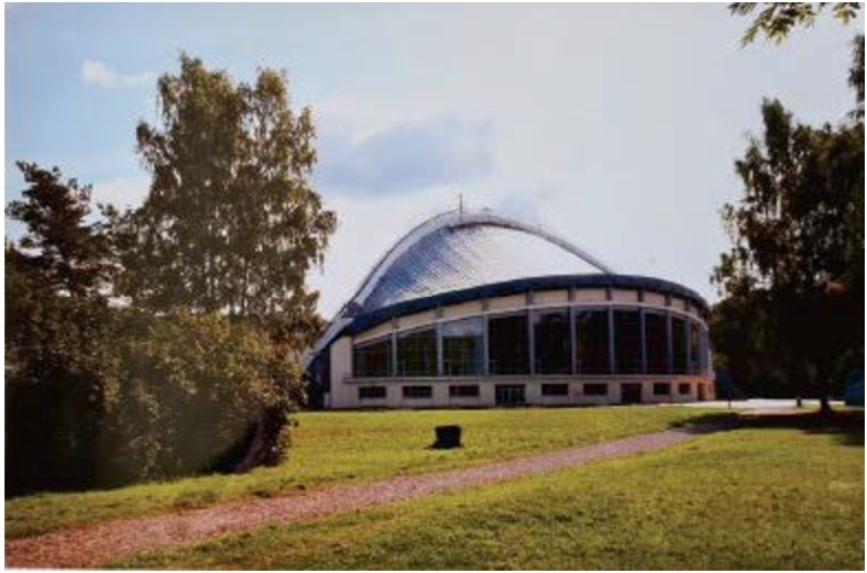
In Lithuania, there are also quite a few buildings with minimal surface elements. The roof of the well-known Vingis Park stage is an almost exactly minimal surface (Fig. 19). The stage was built in 1960 according to the project of Estonian architects A. Kotli, and H. Seppmann, which was implemented a little earlier in Tallinn. The roof of this building is not an exact minimal surface, but in many aspects, it is close to it.
In Lithuania, decorative minimal surface roofs have appeared in Vilnius and Palanga in recent years. Most of them are seasonal café pavilions (Fig. 20). Of the stationary buildings, Palanga Arts and Entertainment Club “Kupeta” should be mentioned separately, which was created and built by UAB “Vingida”.
Fig. 20
Vilnius, Vokiečiu̧ str. Roofs of cafes installed for the summer season, 2009. Photo: M. Sapagovas.
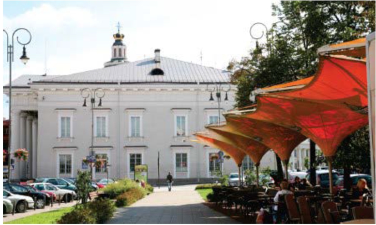
Fig. 21
Shapes of minimal surfaces in lipids. Prof. V. Razumas (Institute of Biochemistry of LAS), 2009. From M. Sapagovas’s photo collections.
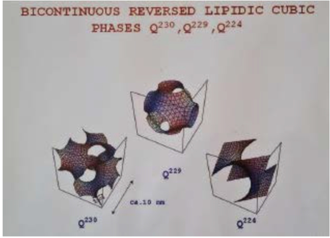
Fig. 22
Minimal surface structures designed by scientists and engineers from Kyiv and Vilnius, 1967–1970.
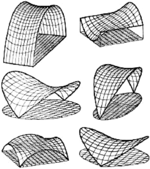
Fig. 23
The six-leaf clover is another example of joint research by Lithuanian mathematicians and Kyiv engineers.
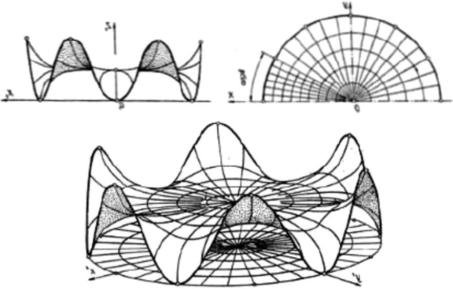
Fig. 24
Spatial shelf “Exept” at Litexpo exhibition, 1998. Designer P. Gasūnas. Photo: M. Sapagovas.
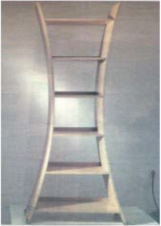
Fig. 25
Flower table. 2009. Photo: M. Sapagovas.

In the 1960s, architects and engineers of the Kyiv Institute of Civil Engineering became interested in minimal surface structures and offered the Numerical Methods Department of the Institute of Physics and Mathematics of the Lithuanian Academy of Sciences to cooperate in designing buildings with this kind of roof. Speaking in architectural terms, Lithuanian mathematicians carried out virtual modelling of building structures. In Kyiv and Cherkasy (there was a branch of the Institute of Civil Engineering in Kyiv), architects planned the possible contours of minimal surfaces (they indicated the domain of definition of the differential equation, as well as the possible boundary conditions), while in Vilnius mathematicians solved the equation of the minimal surface. In this way, many variants of minimal surfaces were analysed together (Figs. 22, 23) (Agalcev and Sapagovas, 1967; Sapagovas, 1984).
Fig. 26
Coffee cups decorated with architectural objects of minimal surfaces. Photo: M. Sapagovas.
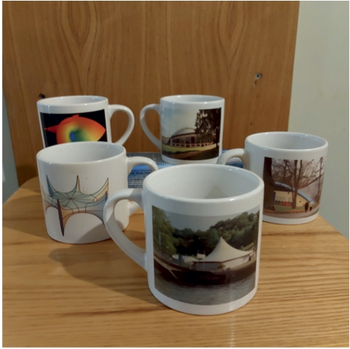
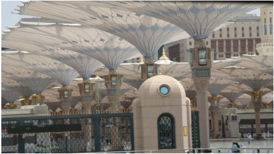
Fig. 28
Choreographic clothing with minimal surface design. Photo from the celebratory concert of the information technology company “Baltic Amadeus”, 2018. From M. Sapagovas’s photo collections.
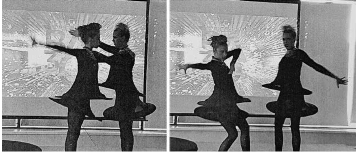
Fig. 29
A. Kasuba. Shelter on Roof Deck. 1974.
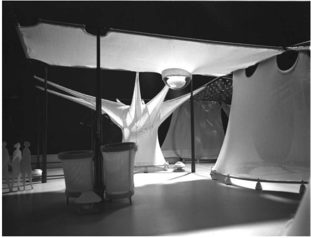
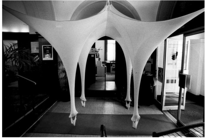
Fig. 30
A. Kasuba. Elements of the Rain Colonnades, 1977.
The mathematical concept of the minimal surface has fascinating applications in biochemistry, particularly in explaining the self-organisation and structural stability of biomolecules and cellular membranes. These surfaces are used to model and analyse various phenomena related to molecular interaction, cell membranes, and protein folding. Amphiphilic molecules (e.g. lipids or their derivatives) in water can form bicontinuous cubic phases (Fig. 21). Their structure is unusually symmetric, containing all combinations of symmetry elements common in crystallography. These microstructures are usually described in terms of differential geometry and minimal surfaces (Hyde et al., 1997; Razumas, 2005; Larsson, 2005). Lithuanian biochemists concentrated on the three main topics, related to the minimal surfaces: 1. Structural features of the protein-containing cubic phases of lipids. 2. Molecular features of the lipid/protein/water cubic phases as revealed by spectroscopic methods. 3. Electrochemical and bioanalytical applications of the cubic phases with entrapped proteins. The third topic was pioneered by the Lithuanian scientists (Razumas, 2005; Valldeperas et al., 2019).
In the book by Prof. Juozas Burneika (1929–2016), considerable attention is paid to the role of minimal surfaces in visual arts (Burneika, 2002). Even in household objects created by Lithuanian designers, minimal surface shapes and images can be found (Figs. 24–26, 28).
In the world of science and art, scientists and artists are constantly emerging who, inspired by the secrets and beauty of minimal surfaces, become real enthusiasts of these surfaces. We have already briefly mentioned one of them, the German architect Frei Otto. His student Mahmoud Bodo Rasch designed a mosque built at the end of the last century in Medina, Saudi Arabia, which is full of philosophically meaningful forms of minimal surfaces (Fig. 27).
Another fan of minimal surfaces is the mathematician Anatoly Fomenko, a professor at Lomonosov University in Moscow, who obtained valuable theoretical results on minimal surfaces by solving the multidimensional Plateau problem (Fomenko, 1989). An original artist, he paints pictures of realistic and imaginary shapes and illustrates books and proofs of geometry theorems with fascinating minimal surfaces.
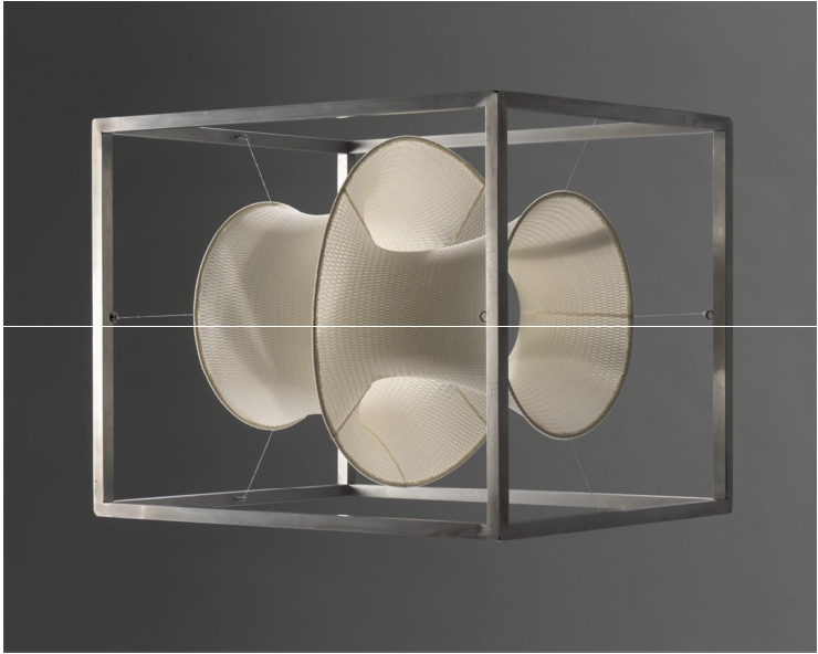
Following the principles of minimalism, Lithuanian American sculptor, ceramicist, and architect Aleksandra Kašubienė (Kasuba) made Lithuania famous with her works (Kasuba, 2019). Alongside her monumental artwork, A. Kašubienė also embodied the principles of minimalism in abstract installations of elastic synthetic fabric, which the artist was encouraged to create by the theory of minimal surfaces and computer technology. From a mathematical point of view, A. Kašubienė, experimenting with rigid tensioned membranes and elastic materials stretched on a spatial contour, created physical models of the minimal surfaces (Figs. 7, 29–33). Not a few of her artworks were created by the following methodology: according to the contour chosen by the artist, researchers in computational mathematics D. Hoffman, J. Hoffman, and W. Meeks III, after solving the minimal surface equation, presented a coloured two-dimensional image of the solution on-screen. Using this image, the A. Kašubienė created spatial models of the surfaces. This cooperation was described in “The New York Times” in 1986.
Fig. 31
A. Kasuba. Whiz Bang Quick City 2. Installation, May 26–June 4, 1972. Woodstock, NY.
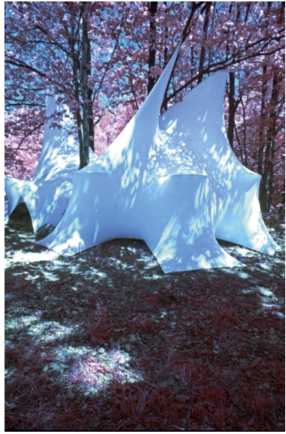
Fig. 32
A. Kasuba. Structures, 1977.
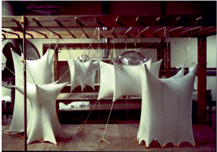
Fig. 33
A. Kasuba. Spectrum, An Afterthought. Model, 1975. Photo: A. Lukšėnas.
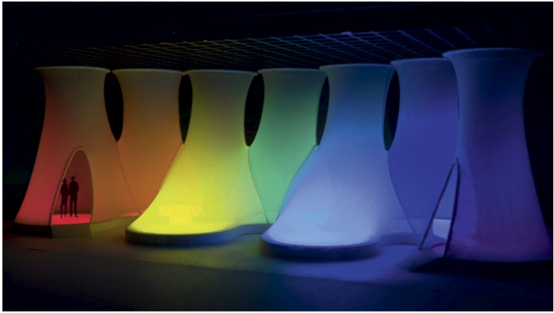
Fig. 34
A. Kasuba. Shell Dwellings. Rock Hill Guest Kitchen, Studio and Bedroom, New Mexico.2003–2005.
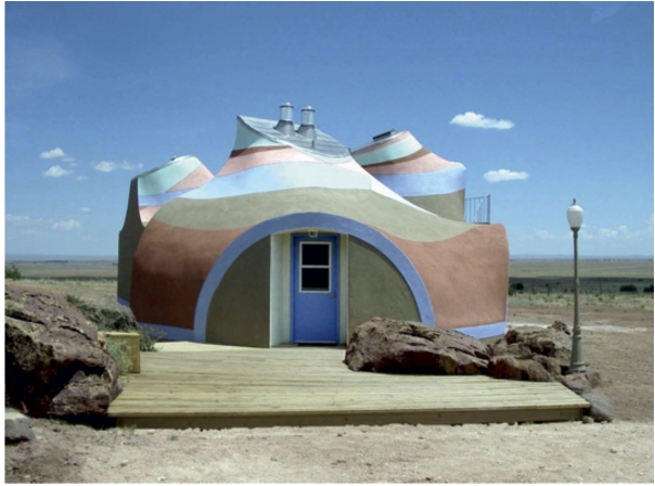
Fig. 35
Aquarium at the Oceanographic Museum in Monaco, 2008. From M. Sapagovas’s photo collections.
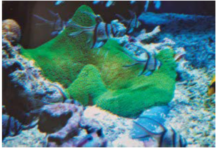
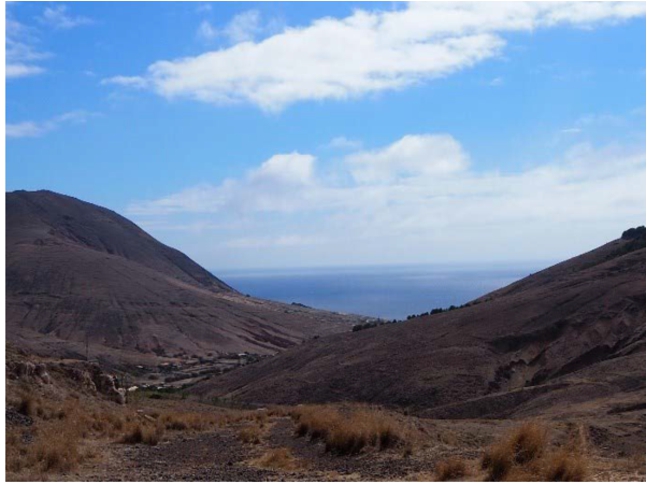
Fig. 36
Porto Santo Island of the Madeira Archipelago. From M. Sapagovas’s photo collections.
In the last years of her life, A. Kašubienė returned from the big city to the shelter of nature and brought to life her childhood vision of buildings without angles. She acquired a piece of land in New Mexico, where she built a residential house and a guest studio with a minimal surface-shaped roof (Fig. 34).
Instead of an Epilogue
The term “minimal surface” is just a man-made construct, a theoretical concept that reflects what nature created a long time ago. A mathematician studying these surfaces is always pleased to notice a saddle-shaped colony of molluscs in an aquarium or a mountain ridge when travelling and once again make sure that natural phenomena obey the laws of minimal form and minimal energy (Figs. 35, 36), while a human can understand what nature brought into being and rationally complement the creations of nature.
Notes
1 Digital images Fig. 7 and Fig. 33 are stored in The Lithuanian National Museum of Art; Figs. 29–32 and Fig. 34 are stored in the Digital Archive of Aleksandra’ Kasuba, The Lithuanian National Museum of Art (Skaitmeniniame Aleksandros Kasubos archyve Lietuvos nacionaliniame dailės muziejuje, SAKA LNDM).
Acknowledgements
The authors are grateful to the Lithuanian National Museum of Art for the opportunity to publish digital images of A. Kasuba’s works.
References
1 | Agalcev, A., Sapagovas, M. ((1967) ). The solution of the equation of minimal surface by finite-difference method. Lithuanian Mathematical Journal, 7: (3), 373–379 (in Russian). https://doi.org/10.15388/LMJ.1967.19976. |
2 | Ambrazevičius, A. ((1981) ). Solvability of the problem in a conical capillary. Problems of mathematical analysis, 8: , 3–23. |
3 | Ambrazevičius, A.P. ((1991) ). Finding the form of the surface of a liquid in a conical container for a given volume of the liquid. I. Lithuanian Mathematical Journal, 22: (1), 1–6. https://doi.org/10.1007/BF00967921. |
4 | Burneika, J. ((2002) ). Forma, kompozicija, dizainas. VDA leidykla. |
5 | Concus, P. ((1967) ). Numerical solution of the minimal surface equation. Mathematics of Computation, 21: (99), 340–350. https://doi.org/10.2307/2003235. |
6 | Čiupaila, R., Sapagovas, M. ((2002) ). Solution of the system of parametric equations of the sessile drop. Nonlinear Analysis: Modelling and Control, 7: (2), 201–206. https://doi.org/10.3846/13926292.2002.9637192. |
7 | Čiupaila, R., Sapagovas, M., Štikonienė, O. ((2013) ). Numerical solution of nonlinear elliptic equation with nonlocal condition. Nonlinear Analysis: Modelling and Control, 18: (4), 412–426. https://doi.org/10.15388/NA.18.4.13970. |
8 | Douglas, J. ((1927–1928) ). A method of numerical solution of the problem of Plateau. Annals of Mathematics, 29: (1/4), 180–188. https://doi.org/10.2307/1967991. |
9 | Drew, P. ((1976) ). Frei Otto: Form and Structure. Westview Press. |
10 | Fomenko, A.T. ((1989) ). The Plateau Problem: Historical Survey. Gordon & Breach, Williston, VT. |
11 | Glotov, D., Hames, W.E., Meir, A.J., Ngoma, S. ((2016) ). An integral constrained parabolic problem with applications in thermochronology. Computers & Mathematics with Applications, 71: (11), 2301–2312. https://doi.org/10.1016/j.camwa.2016.01.017. |
12 | Greenspan, D. ((1965) ). On approximating extremals of functionals. Part I. The method and examples for boundary value problems. International Computing Centre Bulletin, University of Roma, 4: , 99–120. |
13 | Halbrecht, H. ((2009) ). On the numerical solution of Plateau’s problem. Applied Numerical Mathematics, 59: (11), 2785–2800. https://doi.org/10.1016/j.apnum.2008.12.028. |
14 | Hyde, S., Andersson, S., Larsson, K., Blum, Z., Landh, T., Lidin, S., Ninham, B.W. ((1997) ). The Language of Shape. The Role of Curvature in Condensed Matter: Physics, Chemistry and Biology. Elsevier, Amsterdam. |
15 | Johnson, C., Thomée, V. ((1975) ). Error estimation for a finite element approximation of a minimal surface. Mathematics of Computation, 29: (130), 343–349. https://doi.org/10.2307/2005555. |
16 | Kasuba, A. ((2019) ). Kasuba Works. https://www.kasubaworks.com. |
17 | Larsson, K. ((2005) ). In: Lynch, M.L., Spicer, P.T. (Eds.) Bicontinuous Liquid Crystals. CRC Press Taylor & Francis Group, Boca Raton, USA, pp. 3–13. Chapter 1. Bicontinuous cubic liquid crystalline materials: a historical perspective and modern assessment. |
18 | Lipkovski, J., Lipkovski, A. ((2015) ). Form-finding software and minimal surface equation: a comparative approach. Filomat, 29: (10), 2447–2455. https://doi.org/10.2298/FIL1510447L. |
19 | Otto, F., Rasch, B. ((1996) ). Finding Form: Towards an Architecture of the Minimal. Axel Menges. |
20 | Pan, Q., Xu, G. ((2011) ). Construction of minimal subdivision surface with a given boundary. Computer-Aided Design, 43: (4), 374–380. https://doi.org/10.1016/j.cad.2010.12.013. |
21 | Ragulskis, K., Sapagovas, M., Čiupaila, R., Jurkulnevičius, A. ((1986) ). Numerical experiment in stationary problems of liquid metal contact. Vibrotechnika, 4: (57), 105–111. |
22 | Razumas, V. ((2005) ). In: Lynch, M.L., Spicer, P.T. (Eds.) Bicontinuous Liquid Crystals. CRC Press Taylor & Francis Group, Boca Raton, USA, pp. 169–211. Chapter 7. Bicontinuous cubic phases of lipids with entrapped proteins: structural features and bioanalytical applications. |
23 | Sakakibara, K., Shimizu, Y. (2022). Numerical analysis for the Plateau problem by the method of fundamental solutions. Numerical Analysis, 1–21. https://doi.org/10.48550/arXiv.2212.06508. |
24 | Sapagovas, M. ((1982) ). The difference method for the solution of the problem of the equilibrium of a drop of liquid. Difference Equations and Their Applications, 31: , 63–72 (in Russian). |
25 | Sapagovas, M. ((1983) ). Numerical methods for the solution of the equation of a surface with prescribed mean curvature. Lithuanian Mathematical Journal, 23: (3), 321–326. https://doi.org/10.1007/BF00966474. |
26 | Sapagovas, M. (1984). Difference Methods for Solution of Nonlinear Elliptic Equations. Doctor thesis, M.V. Keldysh Institute of Applied Mathematics, Moscow. |
27 | Sapagovas, M. ((2023) ). Plateau problem and minimal surfaces: numerical methods and applications. Lietuvos matematikos rinkinys. LMD darbai, ser. B, 64: , 1–15 (in Lithuanian). https://doi.org/10.15388/LMR.2023.33611. |
28 | Schumacher, H., Wardetzky, M. ((2019) ). Variational convergence of discrete minimal surfaces. Numerische Mathematik, 141: , 173–213. https://doi.org/10.1007/s00211-018-0993-z. |
29 | Tråsdahl, Ø., Rønquist, E.M. ((2011) ). High order numerical approximation of minimal surfaces. Journal of Computational Physics, 230: (11), 4795–4810. |
30 | Uraltseva, N.N. (1973). Solution of the capillarity problem. Vestnik, Leningrad University. Mathematics, (19), 54–64. |
31 | Valldeperas, M., Salis, A., Barauskas, J., Tiberg, F., Arnebrant, T., Razumas, V., Monduzzi, M., Nylander, T. ((2019) ). Enzyme encapsulation in nanostructured self-assembled structures: Toward biofunctional supramolecular assemblies. Current Opinion in Colloid & Interface Science, 44: , 130–142. https://doi.org/10.1016/j.cocis.2019.09.007. |
32 | Vogel, T.I. ((1987) ). Stability of a Liquid Drop Trapped Between Two Parallel Planes. SIAM Journal on Applied Mathematics, 47: (3), 516–525. http://www.jstor.org/stable/2101796. |
33 | Zareckas, V.-S.S., Ragulskienė, V.L. ((1971) ). Mercury Switching Elements for Automation Devices. Automation Library. Energy. |


